Economical realization of phase covariant devices in arbitrary dimensions

The possibility of employing quantum systems with (finite) dimension higher than two in quantum information has recently triggered much interest. In particular, it has been shown that an increase in the dimension leads to a better performance of various quantum information protocols, such as for example quantum cryptography qc3; 3dim and some problems in distributed quantum computing gima. Moreover, considerable experimental progress has been recently reported in the generation, manipulation and detection of quantum systems with higher dimension exp.

In this work we consider the case of phase covariant transformations where the information is encoded into phase properties of states with arbitrary finite dimension $d$. Encoding information into phase shifts has important applications in quantum computation and quantum information. For example, it was shown that the existing quantum algorithms can be described in a unified way as quantum interference processes among different computational paths where the result of the computation is retrieved from a phase shift cemm.

We will describe in a unified framework the features of multi users phase covariant transformations in arbitrary dimension $d$, where typically an arbitrary number of input systems $N$ described by the same quantum state is transformed into a larger number of output systems $M$, which are still described by the same output density operators. We will then specify this description to two tasks of interest in quantum information, namely cloning and phase conjugation.

The no cloning theorem no-cloning states the impossibility of perfectly cloning unknown quantum states selected from a nonorthogonal set, and is the basis of the security of quantum cryptography BB84; E91. Approximate quantum cloning has been extensively studied in the last years and has led to relevant results in quantum cryptography. The eavesdropping strategies in quantum key distribution protocols that are known to be optimal so far are actually based on cloning attacks 3dim; bcdm; cbm. Moreover, quantum cloning allows to study the sharing of quantum information among several parties and it may be applied also to study the security of multi-party cryptographic schemes multi-qc.

Perfect phase conjugation of the density operator of an unknown input state, or equivalently ideal time reversal, is also forbidden by the laws of quantum mechanics. Such a transformation has also recently attracted much interest in connection to the problem of entanglement, in regards to the so-called PPT (positive partial transpose) criterion peres; H3. Since phase conjugation cannot be achieved unitarily, one can try to approximate the transformation with a physical channel, optimizing the fidelity of the output state with the complex-conjugated input. In the case of qubits ($d=2$) phase conjugation is unitarily equivalent to the NOT operation univ-not. For the set of all pure states the resulting universal optimal channel is “classical” univ-not; opt-transp, namely, it can be achieved by state-estimation followed by state-preparation. In contrast, as we will show in this work, for equatorial pure states the optimal phase covariant conjugation map is a purely quantum transformation (for any number of input copies), generalising to the case of many copies the analogous result already proved for a single input system phasenot.

The paper is organised as follows. In Sect. II we describe in a unified framework the operation of multi users phase covariant transformations in arbitrary finite dimension $d$. In Sect. III we review the concept of economical maps. In Sects. IV and V we derive the optimal phase covariant cloning and phase conjugation maps respectively for equatorial input states, and show that for some particular relations between the input and output number of copies the optimal transformations can be achieved economically. In Sect. VI we prove a relation between optimal multiple phase estimation procedures and the optimal cloning and phase conjugation maps. In Sect. VII we summarise the results presented in this work. Some technical details of the derivations presented in the paper are explained in the Appendices.

In this paper we consider quantum devices, or channels (i. e. trace-preserving completely positive maps kraus), from states on an input quantum system $\mathscr{H}_{\textrm{in}}$ to states on a generally different output quantum system $\mathscr{H}_{\textrm{out}}$, for which we assume that an underlying global symmetry under the action of the phase rotations group $\mathbb{U}(1)$ holds. More precisely, we will optimise the action of such devices on pure $d$-dimensional input states of the form

where $\{|0\rangle,\dots,|d-1\rangle\}$ is a fixed orthonormal basis of a $d$-dimensional system $\mathscr{H}$, and the $\phi_{j}$’s are $(d-1)$ independent phases in the interval $[0,2\pi)$. Notice that the choice $\phi_{0}=0$ is not restrictive, since an overall phase is negligible. In the case of qubits, i. e. $d=2$, pure states as in Eq. (1) all lie on one equator of the Bloch sphere and they clearly form a set that is invariant under rotations around the fixed axis orthogonal to this equator. These rotations form a group that is isomorphic to the group $\mathbb{U}(1)$. For generic dimensions $d>2$, this geometrical picture is straightforwardly generalized by saying that pure states in Eq. (1) form a set of states that is invariant under the action of the unitary representation $U_{\{\phi_{j}\}}=|0\rangle\langle 0|+\sum_{j=1}^{d-1}|j\rangle\langle j|e^{i\phi_{j}}$ of the group $\mathbb{U}(1)^{\times(d-1)}$. In the following, with a little abuse of terminology, we will call states of the form (1) as equatorial states, also in the case $d>2$. Notice that starting from a fixed state $|\psi_{0}\rangle=d^{-1/2}\sum_{i}|i\rangle$, usually called seed, it is possible to span the whole invariant family by applying the unitary operator $U_{\{\phi_{j}\}}$

Since we are considering input states belonging to phase-rotations-group-invariant families, the natural scenario for our analysis is then the framework of phase covariant channels, namely channels $\mathcal{E}$ that automatically propagate to the output the action of the group on the input as follows

where $V_{g}$ and $W_{g}$ are unitary representations of $\mathbb{U}(1)^{\times(d-1)}$ on the input and output space, respectively. More explicitly, when the input consists of $N$ copies of an unknown pure equatorial state, i. e. $|\psi(\{\phi_{j}\})\rangle^{\otimes N}$, we have $V_{g}=V_{\{\phi_{j}\}}=U_{\{\phi_{j}\}}^{\otimes N}$. The choice of the output representation $W_{g}$ will depend on the task we want to optimize. For the moment, just notice that both $V_{g}$ and $W_{g}$ are different unitary representations of the same group $\mathbb{U}(1)^{\times(d-1)}$.

Since we are considering only pure input states of the form $|\psi\rangle^{\otimes N}$ we can restrict our attention to channels whose input states have support on the symmetric subspace $\mathscr{H}^{\otimes N}_{+}$ of $\mathscr{H}^{\otimes N}$, that is, $\mathscr{H}_{\textrm{in}}=\mathscr{H}^{\otimes N}_{+}$. Moreover, we require that also the output states have support on the symmetric subspace, namely $\mathscr{H}_{\textrm{out}}=\mathscr{H}^{\otimes M}_{+}\subset\mathscr{H}^{\otimes M}$. In this way it is guaranteed that the output single site density operators are the same. For the following, we choose an orthonormal basis in the symmetric subspace $\mathscr{H}^{\otimes N}_{+}$ of the form

where $P_{\pi}^{(N)}$ denotes a permutation operator of the $N$ systems, $n_{0}$ is the number of systems in state $|0\rangle$, $n_{1}$ in state $|1\rangle$, and so on, with the constraint $\sum_{i=0}^{d-1}n_{i}=N$. The notation $|\{m_{i}\}\rangle_{M}$, with $\sum_{i=0}^{d-1}m_{i}=M$, denotes the analogous symmetric state as in Eq. (4) for the output subspace $\mathscr{H}^{\otimes M}_{+}$. As a convention, in this paper we will consistently use letters $n$’s for the input and $m$’s for the output.

A convenient formalism to deal with covariant channels is the Choi-Jamiołkowski isomorphism jam; choi between completely positive maps $\mathcal{M}$ from states on $\mathscr{H}_{\textrm{in}}$ to states on $\mathscr{H}_{\textrm{out}}$ and positive operators $R_{\mathcal{M}}$ on $\mathscr{H}_{\textrm{out}}\otimes\mathscr{H}_{\textrm{in}}$

where $\mathcal{I}$ is the identity channel and $|\Omega\rangle=\sum_{k=1}^{d}|k\rangle\otimes|k\rangle$ is the (non normalized) maximally entangled vector in the Hilbert space $\mathscr{H}_{\textrm{in}}\otimes\mathscr{H}_{\textrm{in}}$. With the notation introduced in Eq. (4) we have

The correspondence (5) is one-to-one, the inverse formula being

where $\operatorname{Tr}_{\textrm{in}}$ denotes the trace over $\mathscr{H}_{\textrm{in}}$, $\mathbb{I}_{\textrm{out}}$ is the identity matrix over $\mathscr{H}_{\textrm{out}}$, and $\rho^{*}$ is the complex conjugated of $\rho$ with respect to the basis fixed by $|\Omega\rangle$ in Eq. (6). Trace-preservation condition is then given by $\operatorname{Tr}_{\textrm{out}}[R_{\mathcal{M}}]=\mathbb{I}_{\textrm{in}}$.

In terms of the Choi-Jamiołkowski operator, the covariance condition (3) can be rewritten as a commutation relation paolino

where $W_{g}\otimes V_{g}^{*}$ is a new unitary representation of $\mathbb{U}(1)^{\times(d-1)}$. Such a representation is generally reducible, whence, by Schur lemma, $R_{\mathcal{E}}$ splits into a direct sum

where the index $\alpha$ labels the equivalence classes of the one-dimensional onedim irreducible representations of $W_{g}\otimes V_{g}^{*}$. In Sections IV and V we will specialize Eq. (8) to the cases of $N\to M$ cloning and $N\to M$ phase conjugation, for which $W_{g}=U_{\{\phi_{j}\}}^{\otimes M}$ and $W_{g}=\left(U_{\{\phi_{j}\}}^{*}\right)^{\otimes M}$, respectively.

Let $\mathcal{M}$ be a completely positive, trace-preserving map from states on $\mathscr{H}_{\textrm{in}}$ to states on $\mathscr{H}_{\textrm{out}}$. From the Stinespring representation theorem Stinespring, it immediately follows that for every completely positive trace-preserving map it is possible to find an auxiliary quantum system with Hilbert space $\mathscr{L}$ and an isometry $V$ from $\mathscr{H}_{\textrm{in}}$ to $\mathscr{H}_{\textrm{out}}\otimes\mathscr{L}$, $V^{\dagger}V=\mathbb{I}_{\textrm{in}}$, such that

Starting from Eq. (10), it is always possible to construct a unitary interaction $U$ realizing $\mathcal{M}$ ozawa; sc as follows

where $|a\rangle$ is a fixed pure state of a second auxiliary quantum system, say $\mathscr{L}^{\prime}$, such that $\mathscr{H}_{\textrm{in}}\otimes\mathscr{L}^{\prime}=\mathscr{H}_{\textrm{out}}\otimes\mathscr{L}$. The Hilbert spaces $\mathscr{L}$ and $\mathscr{L}^{\prime}$ are generally different, and actually play different physical roles.

We define a trace-preserving completely positive map $\mathcal{M}$ to be economical if and only if it admits a unitary form $U$ as

namely, if and only if the map can be physically realized without discarding—i. e. tracing out—resources. We can simply prove that the only maps admitting an economical unitary implementation $U$ as in Eq. (12) are those for which

for an isometry $V$, $V^{\dagger}V=\mathbb{I}_{\textrm{in}}$. In fact, since $(\mathbb{I}_{\textrm{in}}\otimes\langle a|)U^{\dagger}U(\mathbb{I}_{\textrm{in}}\otimes|a\rangle)=\mathbb{I}_{\textrm{in}}$, $U(\mathbb{I}_{\textrm{in}}\otimes|a\rangle)$ is an isometry from $\mathscr{H}_{\textrm{in}}$ to $\mathscr{H}_{\textrm{out}}\otimes\mathscr{L}$. On the other hand, starting from Eq. (13) and using the Gram-Schmidt method one can extend any isometry $V$ from $\mathscr{H}_{\textrm{in}}$ to $\mathscr{H}_{\textrm{out}}\otimes\mathscr{L}$ to a unitary $U$ on the same output space, and write it in the form $V=U(\mathbb{I}_{\textrm{in}}\otimes|a\rangle)$ for a unit vector $|a\rangle\in\mathscr{L}^{\prime}$, with $\mathscr{H}_{\textrm{in}}\otimes\mathscr{L}^{\prime}=\mathscr{H}_{\textrm{out}}\otimes\mathscr{L}$.

Considering classical resources as free, the most general definition of economical map corresponds to having a random-unitary realization of the form

where $p_{i}\geq 0$, $\sum_{i}p_{i}=1$. Using the same fixed ancilla state $|a\rangle$ for all indeces $i$ is not a loss of generality, since in constructing the operators $U_{i}$’s there is always freedom in the choice of the vector $|a\rangle$. According to this more general definition, all economical maps can always be written as a randomization of the form (13) as follows

In this section we derive the form of quantum channels $\mathcal{C}$ that best approximate the ideal cloning map

with $M>N$, for all possible values $\phi_{j}\in[0,2\pi)$. In this case the choice of the unitary representation on the output space is clearly $W_{g}=U_{\{\phi_{j}\}}^{\otimes M}$. The commutation relation (8) can then be rewritten as

¿From the above equation it follows that $R_{\mathcal{C}}$ splits into the block-form

where each set of values $\{m_{j}\}$ identifies a unique class of equivalent irreducible representations of $U_{\{\phi_{j}\}}^{\otimes M}\otimes(U^{*}_{\{\phi_{j}\}})^{\otimes N}$. The equivalent representations within each class can be conveniently written, using the symmetrization convention as in Eq. (4), as

with $\sum_{i=0}^{d-1}n_{i}=N$ and $\sum_{j=0}^{d-1}m_{j}=M-N$. The multi-index $\{n_{i}\}$ runs over all orthonormal vectors of the symmetrised basis for $\mathscr{H}^{\otimes N}_{+}$. With this notation, Eq. (18) becomes

We now have to adjust the parameters $\left\{r^{\{m_{j}\}}_{\{n^{\prime}_{i}\},\{n^{\prime\prime}_{i}\}}\right\}$ describing a generic channel satisfying the commutation relation (17), in order to shape $R_{\mathcal{C}}$ to optimally approximate the ideal map (16). Such an optimal approximation reasonably maximizes the fidelity $F_{\mathcal{C}}$ between the ideal output, namely $|\psi(\{\phi_{j}\})\rangle^{\otimes M}$, and the actual channel output $\mathcal{C}(|\psi(\{\phi_{j}\})\rangle\langle\psi(\{\phi_{j}\})|^{\otimes N})$. By exploiting the inverse formula (7) and the commutation relation (17), one has

Another commonly adopted figure of merit is the single-site fidelity $F_{\mathcal{C}}^{1}$ between the ideal output $|\psi(\{\phi_{j}\})\rangle$ and the actual single-site output $\operatorname{Tr}_{M-1}[\mathcal{C}(|\psi(\{\phi_{j}\})\rangle\langle\psi(\{\phi_{j}\})|^{\otimes N})]$, namely

We point out that a channel $\mathcal{C}$ maximizing $F_{\mathcal{C}}$ does not necessarily maximize also $F_{\mathcal{C}}^{1}$ keyl-werner; nostro.

When the output number of copies takes the form $M=kd+N$, with $k\in\mathbb{N}$ and $d$ the dimension of $\mathscr{H}$, there exists a unique channel maximizing at the same time both $F_{\mathcal{C}}$ and $F_{\mathcal{C}}^{1}$ pheconclon. Such a channel is described by the positive rank-one operator

where

The corresponding single-site fidelity $F_{\mathcal{C}}^{1}$ takes the form

where, for the sake of symmetry of the formula, we have chosen the multi index $\bar{n}_{j}$ such that $\sum_{j}\bar{n}_{j}=N-1$. In the case $N=1$, the above equation is simplified as

since $\sum_{i\neq j}(k+1)=kd(d-1)+d(d-1)=(d-1)(M+d-1)$. Notice that $F_{\mathcal{C}}^{1}$ is always strictly greater than the analogous optimal fidelity for the universal cloner keyl-werner, that is $F^{1}_{\textrm{univ}}=\frac{2M+d-1}{M(d+1)}$. This is due to the fact that we are now imposing a covariance condition under the action of $\mathbb{U}(1)^{\times(d-1)}$, that is a much looser condition subgroup than imposing covariance under the action of the whole universal group $\mathbb{SU}(d)$, and therefore there is more freedom in adjusting free parameters to obtain better performances.

As a final remark notice that, since $R_{\mathcal{C}}$ is rank-one, the channel $\mathcal{C}$ acts as (this can be simply checked by using the inverse formula (7))

where $V$ is the isometry defined as

According to the definitions of Section III, this implies that $\mathcal{C}$ is an economical map, and therefore it does not require additional resources other than the $(M-N)$ input blank copies in order to be unitarily realized. This is in contrast to what happens in the universal case, for which $M$ additional sytems must be provided opt-transp; cerf besides the $N$ input copies.

Another basic device which is impossible to achieve in the framework of quantum mechanics is the NOT gate, where the Bloch vector of any input states is reversed, or equivalently the phase conjugation operation. In this section we will derive the form of the quantum channels $\mathcal{N}$ that optimally approximate the operation of phase conjugation

with $M>N$, for all possible values $\phi_{j}\in[0,2\pi)$. The case $M=N=1$ has been thoroughly analysed phasenot. In the case of phase conjugation the output unitary representation of $\mathbb{U}(1)^{\times(d-1)}$ must be chosen as $W_{g}=(U^{*}_{\{\phi_{j}\}})^{\otimes M}$ and the commutation relation (8) becomes

As in the case of phase covariant cloning, the above relation implies a decomposition of $R_{\mathcal{N}}$ into the block-form $R_{\mathcal{N}}=\bigoplus_{\{m_{j}\}}R_{\{m_{j}\}}$, where each set of values $\{m_{j}\}$ identifies a unique class of equivalent irreducible representations of $(U^{*}_{\{\phi_{j}\}})^{\otimes(M+N)}$. The equivalent representations within each class can be conveniently written as

with $\sum_{i=0}^{d-1}n_{i}=N$ and $\sum_{j=0}^{d-1}m_{j}=M+N$. It is clear that the previous equation is well defined only when $m_{i}\geq n_{i}$, for all $i$. In the following we will see that, when the analytical optimization is possible, such a condition is always satisfied.

The figure of merit that we will consider to approximate the phase conjugation channel is the single-site fidelity

where

Exploiting cumbersome combinatorial calculations very similar to those reported in previous work pheconclon, it can be shown that, in the case $M=kd-N$, with $k\in\mathbb{N}\geq N$ and $d$ the dimension of $\mathscr{H}$, there exists a unique channel maximizing $F_{\mathcal{C}}^{1}$. Such a channel is described by the positive rank-one operator

where

and it acts as an isometrical embedding

where the isometry $V$ is defined as

Therefore, also the optimal phase conjugation map for output number of copies $M=kd-N$ can therefore be realised economically. Its single-site fidelity $F_{\mathcal{N}}^{1}$ is given by

where $\sum_{j}\bar{n}_{j}=N-1$. Since $\sum_{i\neq j}k=kd(d-1)=(d-1)(M+1)$ in the case $N=1$ the above expression is simplified as

Notice that for qubits $F_{\mathcal{N}}^{1}=F_{\mathcal{C}}^{1}$. This is due to the fact that for equatorial qubits perfect phase conjugation can be achieved unitarily by a $\pi$ rotation along the $x$ axis. Optimal phase conjugation therefore is equivalent to optimal phase covariant cloning followed by such a rotation, which does not decrease the cloning fidelity. In all the other cases with $d>2$, $F_{\mathcal{N}}^{1}$ is always strictly smaller than $F_{\mathcal{C}}^{1}$. Actually, in these cases phase conjugation can be performed only approximately and therefore the global transformation corresponding to a generation of many phase conjugated copies is worse than just cloning them. However, in the limit of large number of output copies, i. e. $M\to\infty$, they both tend to the same limit, as we will show in Section VI.

Both the cloning fidelity $F_{\mathcal{C}}^{1}$ in Eq. (25) and the phase conjugation fidelity $F_{\mathcal{N}}^{1}$ in Eq. (38), in the limit $M\to\infty$, that is, $k\to\infty$ with $M\approx kd$, take the form

The above expression coincides with the single-site fidelity $F_{\mathcal{P}}^{1}$ of optimal phase estimation on $N$ copies of equatorial states multi-phase. For all possible values of $N$ and $M$, the following relations then hold

The above inequalities are illustrated in Figure 1, where the optimal fidelities of phase covariant cloning and phase conjugation are reported for equatorial states with $d=5$ and $N=1$.

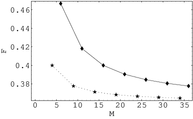
First of all, let us notice that phase covariant conjugation, contrarily to the case of universal transposition opt-transp for which it is known that the optimal strategy trivially consists of an estimation followed by a suitable preparation, achieves a fidelity $F_{\mathcal{N}}^{1}$ that is always greater than the fidelity $F_{\mathcal{P}}^{1}$ achievable by means of a measure-and-prepare scheme. Moreover, Eq. (41) confirms the general fact that cloning fidelity, in the limit of infinite output copies number, tends to state estimation fidelity, and shows that this also holds for other symmetrical covariant devices, such as phase conjugation.

Here we prove that not only the fidelities $F_{\mathcal{C}}^{1}$ and $F_{\mathcal{N}}^{1}$ tend to the phase estimation fidelity $F_{\mathcal{P}}^{1}$, but also that optimal phase covariant cloning $\mathcal{C}$ and phase conjugation $\mathcal{N}$ maps tend, in the limit, to the phase estimation map $\mathcal{P}$ (which estimates the phases $\{\overline{\phi_{j}}\}$ and reprepares the state $|\psi(\{\overline{\phi_{j}}\})\rangle$). This is clearly a much stronger statement than that concerning just fidelities note-on-estim. The main ingredient we need for the proof is that the single-site output state coming from the channel $\mathcal{C}$ can be parametrised by a shrinking parameter $\eta_{\mathcal{C}}$ as

with $\eta_{\mathcal{C}}=(dF_{\mathcal{C}}^{1}-1)/(d-1)$. Analogous formulas hold for phase conjugation $\mathcal{N}$ and phase estimation $\mathcal{P}$, as a consequence of the phase covariant property of the maps (for the explicit calculations, see Appendices A and B).

The proof then goes through a concatenation argument. Imagine to perform an optimal phase estimation multi-phase over $N$ copies of the unknown state $|\psi(\{\phi_{j}\})\rangle$. After obtaining the optimal estimated value $\{\overline{\phi_{j}}\}$ of the phases, it is possible to prepare $M$ copies of the state $|\psi(\{\overline{\phi_{j}}\})\rangle$. This procedure is, by definition, a sub-optimal phase covariant $N\to M$ cloning: the fidelity of such $M$ copies must be smaller than (or at most equal to) the fidelity of the output of an optimal phase covariant cloner, that is

(We put in parentheses the dependence of the fidelities on the input number of copies $N$ and the output number $M$).

The opposite direction can be proved by concatenating the optimal $N\to M$ phase covariant cloner with the optimal state estimation described in References DBE; BM. Since a state estimation implies a phase estimation, it is possible to interpret the whole procedure as a sub-optimal phase estimation: the single-site fidelity $\overline{F}^{1}(N,M)$ obtained in this sub-optimal way must be smaller than or equal to the optimal phase estimation fidelity $F_{\mathcal{P}}^{1}(N)$ for all possible values of $M$. The state estimation map $\mathcal{S}$ works as follows BM

Applying $\mathcal{S}$ to the output of the phase covariant $N\to M$ cloner, we get

Since we assumed that the output state $\rho_{M}$ of a phase covariant cloner has support on the symmetric subspace it can be linearly decomposed as $\rho_{M}=\sum_{i}\lambda_{i}|\psi_{i}\rangle\langle\psi_{i}|^{\otimes M}$ with $\sum_{i}\lambda_{i}=1$ paolo-vittorio. Therefore the above expression can be written as

Noticing that the shrinking factor $\eta_{\mathcal{S}}=M/(M+d)$ BM approaches unit for $M\to\infty$, the last equation implies that

and according to the previous remark about the sub-optimality of this phase estimation procedure, one has

Eq. (48) together with Eq. (43) prove Eq. (41).

The above argument can be applied also to the case of phase conjugation. Actually, a suboptimal phase covariant conjugation map can be achieved by first performing an optimal phase estimation on the input equatorial states, which gives the estimated values $\{\overline{\phi_{j}}\}$ for the phases, and then preparing $M$ copies of the state $|\psi(\{-\overline{\phi_{j}}\})\rangle$. Moreover, a suboptimal phase estimation can be realised by first applying an optimal $N\to M$ phase covariant conjugation device and then performing optimal state estimation on the $M$ output states. In this way we would be able to estimate the $(d-1)$ phase values of the $M$ output states and we would have an estimate of the phases of the $N$ input states just by changing the signs. The comparison of the above two procedures allows to establish the equivalence of optimal phase estimation and optimal phase covariant transposition in the limit of infinite number of output copies.

In this paper we have studied the efficiency of phase covariant multi user channels in arbitrary finite dimension. In particular, we have derived the form of the channels that optimally approach quantum cloning and phase conjugation for multi-phase equatorial states. We have shown that for certain relations between the input and output number of copies the optimal transformations can be achieved economically. We have derived a relation between the above mentioned transformations and optimal multiple phase estimation procedures. In the case of phase conjugation we have shown that, in contrast to the customary case of the Universal-NOT on qubits (or the universal conjugation in arbitrary dimension), the optimal phase covariant transformation for equatorial states is a nonclassical channel, which cannot be achieved via a measurement/preparation procedure.

References

- (1) H. Bechmann-Pasquinucci and A. Peres, Phys. Rev. Lett. 85, 3313 (2000).
- (2) D. Bruß and C. Macchiavello, Phys. Rev. Lett. 88, 127901 (2002); N. Cerf, M. Bourennane, A. Karlsson and N. Gisin, Phys. Rev. Lett. 88, 127902 (2002).
- (3) M. Fitzi, N. Gisin and U. Maurer, Phys. Rev. Lett. 87, 217901 (2002)
- (4) See for example G. Molina-Terriza, A. Vaziri, J. Rehacek, Z. Hradila and A. Zeilinger, Phys. Rev. Lett. 92, 167903 (2004); R. T. Thew, A. Acin, H. Zbinden and N. Gisin, Phys. Rev. Lett. 93, 010503 (2004); R. Das, A. Mitra, V. Kumar S., and A. Kumar, quant-ph/0307240.
- (5) R. Cleve, A. Ekert, C. Macchiavello and M. Mosca, Proc. R. Soc. Lond. A 454, 339, (1998).
- (6) W. K. Wootters and W. H. Zurek, Nature 299, 802 (1982).
- (7) C. H. Bennett and G. Brassard, in Proceedings of the IEEE International Conference on Computers, Systems, and Signal Processing, Bangalore, India, 1984, pp. 175–179.
- (8) A. Ekert, Phys. Rev. Lett. 68, 661 (1991).
- (9) D. Bruß, M. Cinchetti, G. M. D’Ariano, and C. Macchiavello, Phys. Rev. A 62 012302 (2000).
- (10) F. Caruso, H. Bechmann Pasquinucci and C. Macchiavello, Phys. Rev. A 72, 032340 (2005).
- (11) V. Scarani and N. Gisin, J. Phys. A 34 6043 (2001).
- (12) A. Peres, Phys. Rev. Lett. 77, 1413 (1996).
- (13) M. Horodecki, P. Horodecki and R. Horodecki, Phys. Lett. A 232, 333 (1996).
- (14) V. Bužek, M. Hillery, and R. F. Werner, Phys. Rev. A 60, R2626 (1999).
- (15) F. Buscemi, G. M. D’Ariano, P. Perinotti, and M. F. Sacchi, Phys. Lett. A 314, 374 (2003).
- (16) F. Buscemi, G. M. D’Ariano, and C. Macchiavello, Phys. Rev. A 72, 062311 (2005).
- (17) K. Kraus, States, Effects, and Operations: Fundamental Notions in Quantum Theory, Lect. Notes Phys. 190, (Springer-Verlag, 1983).
- (18) A. Jamiołkowski, Rep. Math. Phys. 3, 275 (1972).
- (19) M.-D. Choi, Lin. Alg. Appl. 10, 285 (1975).
- (20) G. M. D’Ariano and P. Lo Presti, Phys. Rev. A 64 042308 (2001).
- (21) The group is commutative, whence its irreducible representations are all one-dimensional.
- (22) W. F. Stinespring, Proc. Am. Math. Soc. 6, 211 (1955).
- (23) M. Ozawa, J. Math. Phys. 5, 848 (1984).
- (24) F. Buscemi, G. M. D’Ariano, and M. F. Sacchi, Phys. Rev. A 68, 042113 (2003).
- (25) M. Keyl and R. F. Werner, J. Math. Phys. 40, 3283 (1999).
- (26) G. M. D’Ariano, and C. Macchiavello, Phys. Rev. A 67, 042306 (2003).
- (27) F. Buscemi, G. M. D’Ariano, and C. Macchiavello, Phys. Rev. A 71, 042327 (2005).
- (28) Actually, is a proper subgroup of .
- (29) T. Durt, J. Fiurasek and N. J. Cerf, Phys. Rev. A 72, 052322 (2005).
- (30) C. Macchiavello, Phys. Rev. A 67, 062302 (2003).
- (31) Recently, it has been proved that cloning channels, in the limit of infinite output copies, tend to measure-and-prepare channels acin. Here, we are able to explicitly show how fast this limit is reached, for every finite .
- (32) J. Bae and A. Acin, quant-ph/0603078.
- (33) R. Derka, V. Bužek, and A. K. Ekert, Phys. Rev. Lett. 80, 1571 (1998).
- (34) D. Bruß and C. Macchiavello, Phys. Lett. A 253, 249 (1999).
- (35) This holds by linearity, since every symmetric operator can be written as a linear combination of -fold tensor product pure states, namely . See Reference symmetric.
- (36) G. M. D’Ariano, V. Giovannetti, and P. Perinotti, J. Math. Phys. 47, 022102 (2006).
- (37) L. Susskind and J. Glogower, Physics 1, 49 (1964).