The Generalized Lyapunov Theorem and its Application to Quantum Channels

Daniel Burgarth¹ Affiliation: ¹Department of Physics & Astronomy, University College London, Gower Street, London WC1E 6BT, UK
²NEST CNR-INFM & Scuola Normale Superiore, Piazza dei Cavalieri 7, I-56126 Pisa, Italy Vittorio Giovannetti² Affiliation: ¹Department of Physics & Astronomy, University College London, Gower Street, London WC1E 6BT, UK
²NEST CNR-INFM & Scuola Normale Superiore, Piazza dei Cavalieri 7, I-56126 Pisa, Italy

Abstract

We give a simple and physically intuitive necessary and sufficient condition for a map acting on a compact metric space to be mixing (i.e. infinitely many applications of the map transfer any input into a fixed convergency point). This is a generalization of the “Lyapunov direct method”. First we prove this theorem in topological spaces and for arbitrary continuous maps. Finally we apply our theorem to maps which are relevant in Open Quantum Systems and Quantum Information, namely Quantum Channels. In this context we also discuss the relations between mixing and ergodicity (i.e. the property that there exist only a single input state which is left invariant by a single application of the map) showing that the two are equivalent when the invariant point of the ergodic map is pure.

I Introduction

Repetitive applications of the same transformation is the key ingredient of many controls techniques. In quantum information processing NIELSEN they have been exploited to inhibit the decoherence of a system by frequently perturbing its dynamical evolution VIOLA1; VIOLA2; VIOLA3; VITALI; SIMON (Bang-Bang control) or to improve the fidelity of quantum gates FRANSON by means of frequent measurements (quantum Zeno-effect PERES). Recently analogous strategies have also been proposed in the context of state preparation KUMMERER; WELLENS; HOMOGENIZATION1; HOMOGENIZATION2; TERHAL; YUASA1; YUASA2 and quantum communication MEMORYSWAP; DUALRAIL; RANDOMRAIL; MULTIRAIL. In Refs. HOMOGENIZATION1; HOMOGENIZATION2 for instance, a homogenization protocol was presented which allows one to transform any input state of a qubit into a some pre-fixed target state by repetitively coupling it with an external bath. A similar thermalization protocol was discussed in Ref. TERHAL to study the efficiency of simulating classical equilibration processes on a quantum computer. In Refs. YUASA1; YUASA2 repetitive interactions with an externally monitored environment were instead exploited to implement purification schemes which would allow one to extract pure state components from arbitrary mixed inputs. An application to quantum communication of similar strategies has been finally given in Refs. MEMORYSWAP; DUALRAIL; RANDOMRAIL; MULTIRAIL where sequences of repetitive operations were used to boost the efficiency of quantum information transmission along spin chains.

The common trait of the proposals KUMMERER; WELLENS; HOMOGENIZATION1; HOMOGENIZATION2; TERHAL; YUASA1; YUASA2; MEMORYSWAP; DUALRAIL; RANDOMRAIL; MULTIRAIL is the requirement that repeated applications of a properly chosen quantum operation $\tau$ converges to a fixed density matrix $x_{*}$ independently from the input state $x$ of the system, i.e.

\displaystyle\tau^{n}(x)\equiv\underbrace{\tau\circ\tau\circ\cdots\circ\tau}_{n}\;(x)\Big|_{n\rightarrow\infty}\longrightarrow\;\;x_{*}\;,

(1)

with “ $\circ$ ” representing the composition of maps. Following the notation of Refs. RAGINSKY; RICHTER we call Eq. (1) the mixing property of $\tau$ . It is related with another important property of maps, namely ergodicity (see Fig. 1). The latter requires the existence of a unique input state $x_{0}$ which is left invariant under a single application of the map¹¹ 1 Definition (2) may sound unusual for readers who are familiar with a definition of ergodicity from statistical mechanics, where a map is called ergodic if its invariant sets have measure 0 or 1. The notion of ergodicity used in the case of a discrete time evolution of a quantum system is different STRICTCONTRATIONS; RAGINSKY. Here, the map $\tau$ is not acting on a measurable space but on the compact convex set of quantum states. A perhaps more intuitive and equivalent definition of ergodicity based on the time average of observables is given by Lemma 5 of the Appendix. , i.e.,

\displaystyle\tau(x)=x\qquad\Longleftrightarrow\qquad x=x_{0}\;.

(2)

Refer to caption — Figure 1: Schematic examples of the orbits of a ergodic and a mixing map.

Ergodicity and the mixing property are of high interest not only in the context of the above quantum information schemes. They also occur on a more fundamental level in statistical mechanics STREATER and open quantum systems OPENQUANTUM; ALICKI, where one would like to study irreversibility and relaxation to thermal equilibrium.

In the case of quantum transformations one can show that mixing maps with convergency point $x_{*}$ are also ergodic with fixed point $x_{0}=x_{*}$ . The opposite implication however is not generally true since there are examples of ergodic quantum maps which are not mixing (see the following). Sufficient conditions for mixing have been discussed both in the specific case of quantum channel TERHAL; RAGINSKY; STRICTCONTRATIONS and in the more abstract case of maps operating on topological spaces STREATER. In particular the Lyapunov direct method STREATER allows one to prove that an ergodic map $\tau$ is mixing if there exists a continuous functional $S$ which, for all points but the fixed one, is strictly increasing under $\tau$ . Here we strengthen this criterion by weakening the requirement on $S$ : our generalized Lyapunov functions are requested only to have limiting values $S(\tau^{n}(x))|_{n\rightarrow\infty}$ which differ from $S(x)$ for all $x\neq x_{0}$ . It turns out that the existence of such $S$ is not just a sufficient condition but also a necessary condition for mixing. Exploiting this fact one can easily generalize a previous result on strictly contractive maps RAGINSKY by showing that maps which are asymptotic deformations (see Definition 6) are mixing. This has, unlike contractivity, the advantage of being a property independent of the choice of metric (see however RICHTER for methods of finding “tight” norms). In some cases, the generalized Lyapunov method permits also to derive an optimal mixing condition for quantum channels based on the quantum relative entropy. Finally a slightly modified version of our approach which employs multi-central Lyapunov functions yields a characterization of (not necessarily mixing) maps which in the limit of infinitely many applications move all points towards a proper subset (rather than a single point) of the input space.

The introduction of a generalized Lyapunov method seems to be sound not only from a mathematical point of view, but also from a physical point of view. In effect, it often happens that the informations available on the dynamics of a system are only those related on its asymptotic behavior (e.g. its thermalization process), its finite time evolution being instead difficult to characterize. Since our method is explicitly constructed to exploit asymptotic features of the mapping, it provides a more effective way to probe the mixing property of the process.

Presenting our results we will not restrict ourself to the case of quantum operations. Instead, following STREATER we will derive them in the more general context of continuous maps operating on topological spaces TOPOLOGYBOOK. This approach makes our results stronger by allowing us to invoke only those hypothesis which, to our knowledge, are strictly necessary for the derivation. It is important to stress however that, as a particular instance, all the Theorems and Lemmas presented in the paper hold for any linear, completely positive, trace preserving map (i.e. quantum channel) operating on a compact subset of normed vectors (i.e. the space of the density matrices of a finite dimensional quantum system). Therefore readers who are not familiar with topological spaces can simply interpret our derivations as if they were just obtained for quantum channels acting on a finite dimensional quantum system.

The paper is organized as follows. In Sec. II the generalized Lyapunov method along with some minor results are presented in the context of topological and metric spaces. Then quantum channels are analyzed in Sec. III providing a comprehensive summary of the necessary and sufficient conditions for the mixing property of these maps. Conclusions and remarks end the paper in Sec. IV.

II Generalized Lyapunov Theorem

II.1 Topological spaces

In this section we introduce the notation and derive our main result (the Generalized Lyapunov Theorem). The properties of Hausdorff, compact and sequentially compact topological spaces will be used TOPOLOGYBOOK. For the sake of readability their definitions and their relations are given in the caption of Fig. 2.

Definition 1.

Let $\mathcal{X}$ be a topological space and let $\tau:\mathcal{X}\rightarrow\mathcal{X}$ be a map. The sequence $x_{n}\equiv\tau^{n}(x)$ , where $\tau^{n}$ is a short-hand notation for the $n-$ fold composition of $\tau,$ is called the orbit of $x.$ An element $x_{*}\in\mathcal{X}$ is called a fixed point of $\tau$ if and only if

\displaystyle\tau(x_{*})=x_{*}\;.

(3)

$\tau$ is called ergodic if and only if it has exactly one fixed point. $\tau$ is called mixing if and only if there exists a convergence point $x_{*}\in\mathcal{X}$ such that any orbit converges to it, i.e.

\displaystyle\lim_{n\rightarrow\infty}x_{n}=x_{*}\quad\forall x\in\mathcal{X}\;.

(4)

Remark.

Here we use the usual topological definition of convergence, i.e. $\lim_{n\rightarrow\infty}x_{n}=x_{*}$ if and only if for each open neighborhood $O(x_{*})$ of $x_{*}$ only finitely many points of the sequence are not in $O(x_{*}).$ This clearly depends on the topology, and there may exist many different points to which a sequence converges to. For example, in the trivial topology of $\mathcal{X}$ where the only open sets are $\mathcal{X}$ and the empty set, any sequence is convergent to any point. On the other hand the uniqueness of the convergence point can be enforced by requiring the topological set $\mathcal{X}$ to be Hausdorff TOPOLOGYBOOK (see Fig. 2 for an explicit definition of this property).

A direct connection between ergodicity and mixing can be established as follows.

Lemma 1.

Let $\tau:\mathcal{X}\rightarrow\mathcal{X}$ be a continuous mixing map on a topological Hausdorff space $\mathcal{X}.$ Then $\tau$ is ergodic.

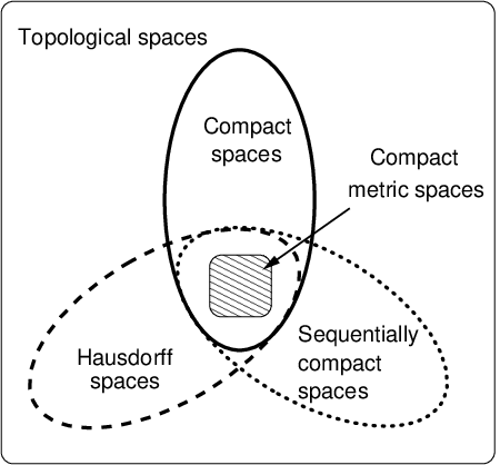
Proof.

Let $x_{*}$ be the convergence point of $\tau$ and let $x\in\mathcal{X}$ arbitrary. Since $\tau$ is continuous we can perform the limit in the argument of $\tau,$ i.e.

\tau(x_{*})=\tau\left(\lim_{n\rightarrow\infty}\tau^{n}(x)\right)=\lim_{n\rightarrow\infty}\tau^{n+1}(x)=x_{*},

which shows that $x_{*}$ is a fixed point of $\tau$ . To prove that it is unique assume by contradiction that $\tau$ possesses a second fixed point $y_{*}\neq x_{*}$ . Then $\lim_{n\rightarrow\infty}\tau^{n}(y_{*})=y_{*}\neq x_{*}$ , so $\tau$ could not be mixing (since the limit is unique in a Hausdorff space – see Fig. 2). Hence $\tau$ is ergodic. ∎

Remark.

The converse is not true in general, i.e. not every ergodic map is mixing (not even in Hausdorff topological spaces). A simple counterexample is given by $\tau:[-1,1]\rightarrow[-1,1]$ with $\tau(x)\equiv-x$ and the usual topology of $\mathbb{R}$ , which is ergodic with fixed point $0,$ but not mixing since for $x\neq 0$ , $\tau^{n}(x)=(-1)^{n}x$ is alternating between two points. A similar counterexample will be discussed in the quantum channel section (see Example 1).

A well known criterion for mixing is the existence of a Lyapunov function STREATER.

Definition 2.

Let $\tau:\mathcal{X}\rightarrow\mathcal{X}$ be a map on a topological space $\mathcal{X}.$ A continuous map $S:\mathcal{X}\rightarrow\mathbb{R}$ is called a (strict) Lyapunov function for $\tau$ around $x_{*}\in\mathcal{X}$ if and only if

S\left(\tau(x)\right)>S(x)\quad\forall x\neq x_{*}.

Remark.

At this point is is neither assumed that $x_{*}$ is a fixed point, nor that $\tau$ is ergodic. Both follows from the theorem below.

Theorem 1 (Lyapunov function).

Let $\tau:\mathcal{X}\rightarrow\mathcal{X}$ be a continuous map on a sequentially compact topological space $\mathcal{X}$ . Let $S:\mathcal{X}\rightarrow\mathbb{R}$ be a Lyapunov function for $\tau$ around $x_{*}.$ Then $\tau$ is mixing with the fixed point $x_{*}$ .

The proof of this theorem is given in STREATER. We will not reproduce it here, because we will provide a general theorem that includes this as a special case. In fact, we will show that the requirement of the strict monotonicity can be much weakened, which motivates the following definition.

Definition 3.

Let $\tau:\mathcal{X}\rightarrow\mathcal{X}$ be a map on a topological space $\mathcal{X}.$ A continuous map $S:\mathcal{X}\rightarrow\mathbb{R}$ is called a generalized Lyapunov function for $\tau$ around $x_{*}\in\mathcal{X}$ if and only if the sequence $S\left(\tau^{n}(x)\right)$ is point-wise convergent for any $x\in\mathcal{X}$ and $S$ fulfills

S_{*}(x)\equiv\lim_{n\rightarrow\infty}S\left(\tau^{n}(x)\right)\neq S(x)\quad\forall x\neq x_{*}.

(5)

In general it may be difficult to prove the point-wise convergence. However if $S$ is monotonic under the action of $\tau$ and the space is compact, the situation becomes considerably simpler. This is summarized in the following Lemma.

Lemma 2.

Let $\tau:\mathcal{X}\rightarrow\mathcal{X}$ be map on a compact topological space. A continuous map $S:\mathcal{X}\rightarrow\mathbb{R}$ which fulfills

S\left(\tau(x)\right)\geqslant S(x)\quad\forall x\in\mathcal{X},

(6)

and

S_{*}(x)\equiv\lim_{n\rightarrow\infty}S\left(\tau^{n}(x)\right)>S(x)\quad\forall x\neq x_{*}.

(7)

for some fixed $x_{*}\in\mathcal{X}$ is a generalized Lyapunov function for $\tau$ around $x_{*}$ .

Proof.

It only remains to show the (point-wise) convergence of $S\left(\tau^{n}(x)\right)$ . Since $S$ is a continuous function on a compact space, it is bounded. By Eq. (6) the sequence is monotonic. Any bounded monotonic sequence converges. ∎

Corollary 1.

Let $\tau:\mathcal{X}\rightarrow\mathcal{X}$ be a map on a compact topological space. A continuous map $S:\mathcal{X}\rightarrow\mathbb{R}$ which fulfills

S\left(\tau(x)\right)\geqslant S(x)\quad\forall x\in\mathcal{X},

and

S\left(\tau^{N}(x)\right)>S(x)\quad\forall x\neq x_{*},

for some fixed $N\in\mathbb{N}$ and for some $x_{*}\in\mathcal{X}$ is a generalized Lyapunov function for $\tau$ around $x_{*}$ .

Remark.

This implies that a strict Lyapunov function is a generalized Lyapunov function (with $N=1$ ).

We can now state the main result of this section:

Theorem 2 (Generalized Lyapunov function).

Proof.

Consider the orbit $x_{n}\equiv\tau^{n}(x)$ of a given $x\in\mathcal{X}.$ Because $\mathcal{X}$ is sequentially compact, the sequence $x_{n}$ has a convergent subsequence (see Fig. 2), i.e. $\lim_{k\rightarrow\infty}x_{n_{k}}\equiv\tilde{x}$ . Let us assume that $\tilde{x}\neq x_{*}$ and show that this leads to a contradiction. By Eq. (5) we know that there exists a finite $N\in\mathbb{N}$ such that

S\left(\tau^{N}(\tilde{x})\right)\neq S(\tilde{x}).

(8)

Since $\tau^{N}$ is continuous we can perform the limit in the argument, i.e. $\lim_{k\rightarrow\infty}\tau^{N}\left(x_{n_{k}}\right)=\tau^{N}(\tilde{x})$ . Likewise, by continuity of $S$ we have

\lim_{k\rightarrow\infty}S\left(x_{n_{k}}\right)=S(\tilde{x}),

(9)

and on the other hand

\lim_{k\rightarrow\infty}S\left(x_{N+n_{k}}\right)=\lim_{k\rightarrow\infty}S\left(\tau^{N}\left(x_{n_{k}}\right)\right)=S(\tau^{N}\tilde{x}),

(10)

where the second equality stems from the continuity of the map $S$ and $\tau^{N}$ . Because $S$ is a generalized Lyapunov function, the sequence $S\left(x_{n}\right)$ is convergent. Therefore the subsequences (9) and (10) must have the same limit. We conclude that $S(\tau^{N}\tilde{x})=S(\tilde{x})$ which contradicts Eq. (8). Hence $\tilde{x}=x_{*}.$ Since we have shown that any convergent subsequence of $\tau^{n}(x)$ converges to the same limit $x_{*}$ , it follows by Lemma 4 of the Appendix that $\tau^{n}(x)$ is converging to $x_{*}.$ Since that holds for arbitrary $x$ , it follows that $\tau$ is mixing. ∎

There is an even more general way of defining Lyapunov functions which we state here for completeness. It requires the concept of the quotient topology TOPOLOGYBOOK.

Definition 4.

Let $\tau:\mathcal{X}\rightarrow\mathcal{X}$ be a map on a topological space $\mathcal{X}.$ A continuous map $S:\mathcal{X}\rightarrow\mathbb{R}$ is called a multi-central Lyapunov function for $\tau$ around $\mathcal{F}\subseteq\mathcal{X}$ if and only if the sequence $S\left(\tau^{n}(x)\right)$ is point-wise convergent for any $x\in\mathcal{X}$ and if $S$ and $\tau$ fulfill the following three conditions: $S$ is constant on $\mathcal{F}$ , $\tau(\mathcal{F})\subseteq\mathcal{F}$ , and

S_{*}(x)\equiv\lim_{n\rightarrow\infty}S\left(\tau^{n}(x)\right)\neq S(x)\quad\forall x\notin\mathcal{F}.

For these functions we cannot hope that the orbit is mixing. We can however show that the orbit is “converging” to the set $\mathcal{F}$ in the following sense:

Theorem 3 (Multi-central Lyapunov function).

Let $\tau:\mathcal{X}\rightarrow\mathcal{X}$ be a continuous map on a sequentially compact topological space $\mathcal{X}.$ Let $S:\mathcal{X}\rightarrow\mathbb{R}$ be a multi-central Lyapunov function for $\tau$ around $\mathcal{F}.$ Let $\varphi:\mathcal{X}\rightarrow\mathcal{X}/\mathcal{F}$ be the continuous mapping into the quotient space (i.e. $\varphi(x)=[x]$ for $x\in\mathcal{X}\backslash\mathcal{F}$ and $\varphi(x)=[\mathcal{F}]$ for $x\in\mathcal{F})$ . Then $\tilde{\tau}:\mathcal{X}/\mathcal{F}\rightarrow\mathcal{X}/\mathcal{F}$ given by $\tilde{\tau}([x])=\varphi\left(\tau\left(\varphi^{-1}([x])\right)\right)$ is mixing with fixed point $[\mathcal{F}]$ .

Proof.

First note that $\tilde{\tau}$ is well defined because $\varphi$ is invertible on $\mathcal{X}/\mathcal{F}\backslash[\mathcal{F}]$ and $\tau(\mathcal{F})\subseteq\mathcal{F},$ so that $\tilde{\tau}([\mathcal{F}])=[\mathcal{F}]$ . Since $\mathcal{X}$ is sequentially compact, the quotient space $\mathcal{X}/\mathcal{F}$ is also sequentially compact. Note that for $O$ open, $\tilde{\tau}^{-1}(O)=\varphi\left(\tau^{-1}\left(\varphi^{-1}\left(O\right)\right)\right)$ is the image of $\varphi$ of an open set in $\mathcal{X}$ and therefore (by definition of the quotient topology) open in $\mathcal{X}/\mathcal{F}.$ Hence $\tilde{\tau}$ is continuous. The function $\tilde{S}([x]):\mathcal{X}/\mathcal{F}\rightarrow\mathcal{X}/\mathcal{F}$ given by $\tilde{S}([x])=S(\varphi^{-1}([x]))$ is continuous and easily seen to be a generalized Lyapunov function around $[\mathcal{F}].$ By Theorem 2 it follows that $\tilde{\tau}$ is mixing. ∎

II.2 Metric spaces

We now show that for the particular class of compact topological sets which posses a metric, the existence of a generalized Lyapunov function is also a necessary condition for mixing. In this context the convergence of a sequence is defined with respect to the distance function $d(\cdot,\cdot):\mathcal{X}\times\mathcal{X}\rightarrow\mathbb{R}$ on the space, so that for instance Eq. (3) requires $\lim_{n\rightarrow\infty}d(x_{n},x_{*})=0$ .

Theorem 4 (Lyapunov criterion).

Let $\tau:\mathcal{X}\rightarrow\mathcal{X}$ be a continuous map on a compact metric space $\mathcal{X}.$ Then $\tau$ is mixing with fixed point $x_{*}$ if and only if a generalized Lyapunov function around $x_{*}$ exists.

Proof.

Firstly, in metric spaces compactness and sequential compactness are equivalent, so the requirements of Theorem 2 are met. Secondly, for any mixing map $\tau$ with fixed point $x_{*},$ a generalized Lyapunov function around $x_{*}$ is given by $S(x)\equiv d(x_{*},x)$ . In fact, it is continuous because of the continuity of the metric and satisfies

\lim_{n\rightarrow\infty}S\left(\tau^{n}(x)\right)=d(x_{*},x_{*})=0\leqslant d(x_{*},x)=S(x),

where the equality holds if and only $x=x_{*}.$ We call $d(x_{*},x)$ the trivial generalized Lyapunov function. ∎

Remark.

In the above Theorem we have not used all the properties of the metric. In fact a continuous semi-metric (i.e. without the triangle inequality) would suffice.

The trivial Lyapunov function requires knowledge of the fixed point of the map. There is another way of characterizing mixing maps as those which bring elements closer to each other (rather than closer to the fixed point).

Definition 5.

A map $\tau:\mathcal{X}\rightarrow\mathcal{X}$ is on a metric space is called a non-expansive map if and only if

d(\tau(x),\tau(y))\leqslant d(x,y)\quad\forall x,y\in\mathcal{X},

a weak contraction if and only if

d(\tau(x),\tau(y))<d(x,y)\quad\forall x,y\in\mathcal{X},\,x\neq y,

and a strict contraction if and only if there exists a $k<1$ such that

d(\tau(x),\tau(y))\leqslant k\,d(x,y)\quad\forall x,y\in\mathcal{X}\,.

Remark.

The notation adopted here is slightly different from the definitions adopted by other Authors RAGINSKY; RUSKAI; WERNER who use contraction to indicate our non-expansive maps. Our choice is motivated by the need to clearly distinguish between non-expansive transformation and weak contractions.

We can generalize the above definition in the following way:

Definition 6.

A map $\tau:\mathcal{X}\rightarrow\mathcal{X}$ on a metric space is called an asymptotic deformation if and only if the sequence $d(\tau^{n}(x),\tau^{n}(y))$ converges point-wise for all $x,y\in\mathcal{X}$ and

\lim_{n\rightarrow\infty}d(\tau^{n}(x),\tau^{n}(y))\neq d(x,y)\quad\forall x,y\in\mathcal{X},\,x\neq y.

Remark.

Let $\tau:\mathcal{X}\rightarrow\mathcal{X}$ be a non-expansive map on a metric space $\mathcal{X},$ and let

\lim_{n\rightarrow\infty}d(\tau^{n}(x),\tau^{n}(y))<d(x,y)\quad\forall x,y\in\mathcal{X},\,x\neq y.

Then $\tau$ is an asymptotic deformation. Any weak contraction is an asymptotic deformation.

Theorem 5 (Asymptotic deformations).

Let $\tau:\mathcal{X}\rightarrow\mathcal{X}$ be a continuous map on a compact metric space $\mathcal{X}$ with at least one fixed point. Then $\tau$ is mixing if and only if $\tau$ is an asymptotic deformation.

Proof.

Firstly assume that $\tau$ is an asymptotic deformation. Let $x_{*}$ be a fixed point and define $S(x)=d(x_{*},x).$

	$\displaystyle\lim_{n\rightarrow\infty}S(\tau^{n}(x))$	$\displaystyle=$	$\displaystyle\lim_{n\rightarrow\infty}d(x_{*},\tau^{n}(x))$
		$\displaystyle=$	$\displaystyle\lim_{n\rightarrow\infty}d(\tau^{n}(x_{}),\tau^{n}(x))\neq d(x_{},x)=S(x)\quad\forall x\neq x_{*},$

hence $S(x)$ is a generalized Lyapunov function. By Theorem 2 it follows that $\tau$ is mixing. Secondly, if $\tau$ is mixing, then

\lim_{n\rightarrow\infty}d(\tau^{n}(x),\tau^{n}(y))=d(x_{*},x_{*})=0\neq d(x,y)\quad\forall x,y\in\mathcal{X},\,x\neq y,

so $\tau$ is an asymptotic deformation. ∎

Remark.

Note that the existence of a fixed point is assured if $\tau$ is a weak contraction on a compact space STAKGOLD, or if the metric space is convex compact DUGUNDJI. As a special case it follows that any weak contraction $\tau$ on a compact metric space is mixing. This result can be seen as an instance of Banach contraction principle on compact spaces. In the second part of the paper we will present a counterexample which shows that weak contractivity is only a sufficient criterion for mixing (see Example 2). In the context of quantum channels an analogous criterion was suggested in STRICTCONTRATIONS; RAGINSKY which applied to strict contractions. We also note that for weak and strict contractions, the trivial generalized Lyapunov function (Theorem 4) is a strict Lyapunov function.

III Quantum Channels

In this Section we discuss the mixing properties of quantum channels NIELSEN which account for the most general evolution a quantum system can undergo including measurements and coupling with external environments. In this context solving the mixing problem (1) is equivalent to determine if repetitive application of a certain physical transformation will drive any input state of the system (i.e. its density matrices) into a unique output configuration. The relationship between the different mixing criteria one can obtain in this case is summarized in Fig. 3.

At a mathematical level quantum channels correspond to linear maps acting on the density operators $\rho$ of the system and satisfying the requirement of being completely positive and trace preserving (CPT). For a formal definition of these properties we refer the reader to KRAUS; WERNER; KEYL: here we remind only that a necessary and sufficient conditions to being CPT is to allow Kraus decomposition KRAUS or, equivalently, Stinespring dilation STINE. Our results are applicable if the underlying Hilbert space is finite dimensional. In such regime there is no ambiguity in defining the convergence of a sequence since all operator norms are equivalent (i.e. given two norms one can construct an upper and a lower bound for the first one by properly scaling the second one). Also the set of bounded operators and the set of operators of Hilbert-Schmidt class coincide. For the sake of definiteness, however, we will adopt the trace-norm which, given the linear operator $\Theta:\mathcal{H}\rightarrow\mathcal{H}$ , is defined as $\|\Theta\|_{1}=\mbox{Tr}[\sqrt{\Theta^{{\dagger}}\Theta}]$ with $\mbox{Tr}[\cdots]$ being the trace over $\mathcal{H}$ and $\Theta^{{\dagger}}$ being the adjoint of $\Theta$ . This choice is in part motivated by the fact RUSKAI that any quantum channel is non-expansive with respect to the metric induced²² 2 This is just the trace distance $d(\rho,\sigma)=\|\rho-\sigma\|_{1}$ . by $\|\cdot\|_{1}$ (the same property does not necessarily apply to other operator norms, e.g. the Hilbert-Schmidt norm, also when these are equivalent to $\|\cdot\|_{1}$ ).

We start by showing that the mixing criteria discussed in the first half of the paper do apply to the case of quantum channels. Then we will analyze these maps by studying their linear extensions in the whole vector space formed by the linear operators of $\mathcal{H}$ . Similar questions also arise in the context of finitely correlated states, where one investigates the decay of correlations in space (rather than in time) FANNES.

III.1 Mixing criteria for Quantum Channels

Let $\mathcal{H}$ be a finite dimensional Hilbert space and let $\mathcal{S}(\mathcal{H})$ be the set of its density matrices $\rho$ . The latter is a convex and compact subspace of the larger normed vector space $\mathcal{L}(\mathcal{H})$ composed by the linear operators $\Theta:\mathcal{H}\rightarrow\mathcal{H}$ of $\mathcal{H}$ . From this and from the fact that CPT maps are continuous (indeed they are linear) it follows that for a quantum channel there always exists at least one density operator which is a fixed point TERHAL. It also follows that all the results of the previous section apply to quantum channels. In particular Lemma 1 holds implying that any mixing quantum channel must be ergodic. The following example shows however that it is possible to have ergodic quantum channels which are not mixing.

Example 1.

Theorems 5 implies that a quantum channel $\tau:\mathcal{S}(\mathcal{H})\rightarrow\mathcal{S}(\mathcal{H})$ is mixing if and only if it is an asymptotic deformation. As already pointed out in the introduction, this property is metric independent (as opposed to contractivity). Alternatively, if the fixed point of a quantum channel is known, then one may use the trivial generalized Lyapunov function (Theorem 4) to check if it is mixing. However both criteria depend on the metric distance, which usually has no easy physical interpretation. A more useful choice of the is the quantum relative entropy, which is defined as

\displaystyle H(\rho,\sigma)\equiv\textrm{Tr}\rho(\log\rho-\log\sigma).

(11)

As discussed in JENS, the quantum relative entropy is continuous in finite dimension and can be used as a measure of ”distance” (though it is not a metric). It is finite if the support of $\rho$ is contained in the support of $\sigma$ . To ensure that it is a continuous function on a compact space, we consider the case when $\sigma$ is faithful:

Theorem 6 (Relative entropy criterion).

A quantum channel with faithful fixed point $\rho_{*}$ is mixing if and only if the quantum relative entropy with respect to $\rho_{*}$ is a generalized Lyapunov function.

Proof.

Because of Theorem 2 we only need to prove the second part of the thesis, i.e. that mixing channels admit the quantum relative entropy with respect to the fixed point, $S(\rho)\equiv H(\rho,\rho_{*})$ , as generalized Lyapunov function. Firstly notice that the quantum relative entropy is monotonic under quantum channels RUSKAI2. Therefore the limit $S_{*}(\rho)\equiv\lim_{n\rightarrow\infty}S\left(\tau^{n}(\rho)\right)$ does exist and satisfies the condition $S_{*}(\rho)\geqslant S(\rho)$ . Suppose now there exists a $\rho$ such that $S_{*}(\rho)=S(\rho)$ . Because $\tau$ is mixing and $S$ is continuous we have

S(\rho)=S_{*}(\rho)=\lim_{n\rightarrow\infty}S\left(\tau^{n}(\rho)\right)=S(\rho_{*})=0,

and hence $H(\rho,\rho_{*})=0$ . Since $H(\rho,\sigma)=0$ if and only if $\rho=\sigma$ it follows that $S$ is a Lyapunov function around $\rho_{*}$ . ∎

Corollary 2 (Unital channels).

A unital channel is mixing if and only if the von Neumann entropy is a generalized Lyapunov function.

Another sufficient condition for mixing is weak contractivity. As already mentioned in the previous section, unfortunately this not a necessary condition. Here we present an explicit counterexample based on a quantum channel introduced in Ref. TERHAL.

Example 2.

\|\;\tau(|2\rangle\langle 2|)-\tau(|0\rangle\langle 0|)\;\|_{1}=\|\;|1\rangle\langle 1|-|0\rangle\langle 0|\;\|_{1}=\|\;|2\rangle\langle 2|-|0\rangle\langle 0|\;\|_{1}\;,

where in the last identity we used the invariance of $\|\cdot\|_{1}$ with respect to unitary transformations.

III.2 Beyond the density matrix operator space: spectral properties

Exploiting linearity quantum channels can be extended beyond the space $\mathcal{S}(\mathcal{H})$ of density operators to become maps defined on the full vector space $L(\mathcal{H})$ of the linear operators of the system, in which basic linear algebra results hold. This allows one to simplify the analysis even though the mixing property (1) is still defined with respect to the density operators of the system.

Mixing conditions for quantum channels can be obtained by considering the structure of their eigenvectors in the extended space $\mathcal{L}(\mathcal{H})$ . For example, it is easily shown that the spectral radius HORNJOHNSON of any quantum channel is equal to unity TERHAL, so its eigenvalues are contained in the unit circle. The eigenvalues $\lambda$ on the unit circle (i.e. $|\lambda|=1$ ) are referred to as peripheral eigenvalues. Also, as already mentioned, since $\mathcal{S}(\mathcal{H})$ is compact and convex, CPT maps have always at least one fixed point which is a density matrix TERHAL. A well-known connection between the mixing properties and the spectrum is given by the

Theorem 7 (Spectral gap criterion).

A quantum channel is mixing if and only if its only peripheral eigenvalue is $1$ and this eigenvalue is simple.

Proof.

The “if” direction can be found in linear algebra textbooks (see for example (HORNJOHNSON, Lemma 8.2.7). Now let us assume that $\tau$ is a mixing quantum channel with fixed point $\rho_{*}$ . Let $\Theta$ be a generic operator in $\mathcal{L}(\mathcal{H})$ . Then $\Theta$ can be decomposed in a finite set of non-orthogonal density operators³³ 3 To show that this is possible, consider an arbitrary operator basis of $\mathcal{L}(\mathcal{H})$ . If $N$ is the finite dimension of $\mathcal{H}$ the basis will contain $N^{2}$ elements. Each element of the basis can then be decomposed into two Hermitian operators, which themselves can be written as linear combinations of at most $N$ projectors. Therefore there exists a generating set of at most $2N^{3}$ positive operators, which can be normalized such that they are quantum states. There even exists a basis (i.e. a minimal generating set), but in general it can not be orthogonalized., i.e. $\Theta=\sum_{\ell}c_{\ell}\rho_{\ell}$ , with $\rho_{\ell}\in\mathcal{S}(\mathcal{H})$ and $c_{\ell}$ complex. Since $\textrm{Tr}\left[\rho_{\ell}\right]=1$ , we have have $\textrm{Tr}\left[\Theta\right]=\sum_{\ell}c_{\ell}$ . Moreover since $\tau$ is mixing we have $\lim_{n\rightarrow\infty}\tau^{n}\left(\rho_{\ell}\right)=\rho_{*}$ for all $\ell$ , with convergence with respect to the trace-norm. Because of linearity this implies

\displaystyle\lim_{n\rightarrow\infty}\tau^{n}\left(\Theta\right)=\sum_{\ell}c_{\ell}\;\rho_{*}=\textrm{Tr}\left[\Theta\right]\;\rho_{*}\;.

(12)

If there existed any other eigenvector $\Theta_{*}$ of $\tau$ with eigenvalue on the unit circle, then $\lim_{n\rightarrow\infty}\tau^{n}(\Theta_{*})$ would not satisfy Eq. (12). ∎

The speed of convergence can also be estimated by TERHAL

\displaystyle\|\tau^{n}\left(\rho\right)-\rho_{*}\|_{1}\;\leqslant C_{N}\;n^{N}\;\kappa^{n}\;,

(13)

where $N$ is the dimensionality of the underlying Hilbert space, $\kappa$ is the modulus of the second largest eigenvalue of $\tau$ , and $C_{N}$ is some constant depending only on $N$ and on the chosen norm. Hence, for $n\gg N$ the convergence becomes exponentially fast. As mentioned in RAGINSKY, the criterion of Theorem 7 is in general difficult to check. This is because one has to find all eigenvalues of the quantum channel, which is hard especially in the high dimensional case. Also, if one only wants to check if a particular channel is mixing or not, then the amount of information obtained is much higher than the required amount.

Example 3.

As an application consider the non mixing CPT map of Example 1. One can verify that apart from the eigenvalue $1$ associated with its fixed point (i.e. the completely mixed state), it possess another peripheral eigenvalue. This is $\lambda=-1$ which is associated with the Pauli operator $|0\rangle\langle 0|-|1\rangle\langle 1|$ .

Corollary 3.

The convergence speed of any mixing quantum channel is exponentially fast for sufficiently high values of $n$ .

Proof.

From Theorem 7 mixing channels have only one peripheral eigenvalue and it is simple. Therefore the derivation of Ref. TERHAL applies and Eq. (13) holds. ∎

This result should be compared with the case of strictly contractive quantum channels whose convergence were shown to be exponentially fast along to whole trajectory RAGINSKY; STRICTCONTRATIONS.

III.3 Ergodic channels with pure fixed points

An interesting class of ergodic quantum channel is formed by those CPT maps whose fixed point is a pure density matrix. Among them we find for instance the maps employed in the communication protocols of Refs. MEMORYSWAP; DUALRAIL; RANDOMRAIL; MULTIRAIL or those of the purification schemes of Refs. YUASA2; YUASA1. We now show that within this particular class, ergodicity and mixing are indeed equivalent properties.

Theorem 8 (Purely ergodic maps).

Let $|\psi_{1}\rangle\langle\psi_{1}|$ be the pure fixed point of an ergodic quantum channel $\tau$ . It follows that $\tau$ is mixing.

Proof.

We will use Theorem 7 showing that $|\psi_{1}\rangle\langle\psi_{1}|$ is the only eigenvector of $\tau$ with peripheral eigenvalue. Assume in fact that $\Theta\in\mathcal{L}(\mathcal{H})$ is a eigenvector of $\tau$ with peripheral eigenvalue, i.e.

\displaystyle\tau\left(\Theta\right)=e^{i\varphi}\Theta\;.

(14)

From Lemma 6 of the Appendix we know that the density matrix $\rho=\sqrt{\Theta\Theta^{{\dagger}}}/g$ , with $g=\mbox{Tr}\left[\sqrt{\Theta^{{\dagger}}\Theta}\right]>0$ , must be a fixed point of $\tau$ . Since this is an ergodic map we must have $\rho=|\psi_{1}\rangle\langle\psi_{1}|$ . This implies $\Theta=g|\psi_{1}\rangle\langle\psi_{2}|$ , with $|\psi_{2}\rangle$ some normalized vector of $\mathcal{H}$ . Replacing it into Eq. (14) and dividing both terms by $g$ yields $\tau\left(|\psi_{1}\rangle\langle\psi_{2}|\right)=e^{i\varphi}|\psi_{1}\rangle\langle\psi_{2}|$ and

\displaystyle|\langle\psi_{1}|\tau(|\psi_{1}\rangle\langle\psi_{2}|)|\psi_{2}\rangle|=1\;.

Introducing a Kraus set $\{K_{n}\}_{n}$ of $\tau$ and employing Cauchy-Schwartz inequality one can then write

$\displaystyle 1$	$\displaystyle=$	$\displaystyle\|\langle\psi_{1}\|\tau(\|\psi_{1}\rangle\langle\psi_{2}\|)\|\psi_{2}\rangle\|=\|\sum_{n}\langle\psi_{1}\|K_{n}\|\psi_{1}\rangle\langle\psi_{2}\|K_{n}^{{\dagger}}\|\psi_{2}\rangle\|$
	$\displaystyle\leqslant$	$\displaystyle\sqrt{\sum_{n}\langle\psi_{1}\|K_{n}\|\psi_{1}\rangle\langle\psi_{1}\|K_{n}^{{\dagger}}\|\psi_{1}\rangle}\sqrt{\sum_{n}\langle\psi_{2}\|K_{n}\|\psi_{2}\rangle\langle\psi_{2}\|K_{n}^{{\dagger}}\|\psi_{2}\rangle}$
	$\displaystyle=$	$\displaystyle\sqrt{\langle\psi_{1}\|\tau(\|\psi_{1}\rangle\langle\psi_{1}\|)\|\psi_{1}\rangle}\sqrt{\langle\psi_{2}\|\tau(\|\psi_{2}\rangle\langle\psi_{2}\|)\|\psi_{2}\rangle}=\sqrt{\langle\psi_{2}\|\tau(\|\psi_{2}\rangle\langle\psi_{2}\|)\|\psi_{2}\rangle}\;,$

where we used the fact that $|\psi_{1}\rangle$ is the fixed point of $\tau$ . Since $\tau$ is CPT the quantity $\langle\psi_{2}|\tau(|\psi_{2}\rangle\langle\psi_{2}|)|\psi_{2}\rangle$ is upper bounded by $1$ . Therefore in the above expression the inequality must be replaced by an identity, i.e.

\displaystyle\langle\psi_{2}|\tau(|\psi_{2}\rangle\langle\psi_{2}|)|\psi_{2}\rangle=1\qquad\Longleftrightarrow\qquad\tau(|\psi_{2}\rangle\langle\psi_{2}|)=|\psi_{2}\rangle\langle\psi_{2}|\;.

Since $\tau$ is ergodic, we must have $|\psi_{2}\rangle\langle\psi_{2}|=|\psi_{1}\rangle\langle\psi_{1}|$ . Therefore $\Theta\propto|\psi_{1}\rangle\langle\psi_{1}|$ which shows that $|\psi_{1}\rangle\langle\psi_{1}|$ is the only peripheral eigenvalue of $\tau$ . ∎

An application of the previous Theorem is obtained as follows.

Lemma 3.

Let $M_{AB}=M_{A}\otimes 1_{B}+1_{A}\otimes M_{B}$ be an observable of the composite system $\mathcal{H}_{A}\otimes\mathcal{H}_{B}$ and $\tau$ the CPT linear map on $\mathcal{H}_{A}$ of Stinespring form STINE

\tau(\rho)=\emph{\mbox{Tr}}_{B}\left[U\left(\rho\otimes|\phi\rangle_{B}\langle\phi|\right)U^{{\dagger}}\right]\;,

(15)

(here $\emph{\mbox{Tr}}_{X}\left[\cdots\right]$ is the partial trace over the system $X$ , and $U$ is a unitary operator of $\mathcal{H}_{A}\otimes\mathcal{H}_{B}$ ). Assume that $\left[M_{AB},U\right]=0$ and that $|\phi\rangle_{B}$ is the eigenvector corresponding to a non-degenerate maximal or minimal eigenvalue of $M_{B}.$ Then $\tau$ is mixing if and only if $U$ has one and only one eigenstate that factorizes as $|\nu\rangle_{A}\otimes|\phi\rangle_{B}.$

Proof.

Let $\rho$ be an arbitrary fixed point of $\tau$ (since $\tau$ is CPT it has always at least one), i.e. $\textrm{Tr}_{B}\left[U\left(\rho\otimes|\phi\rangle_{B}\langle\phi|\right)U^{{\dagger}}\right]=\rho$ . Since $M_{AB}=M_{A}+M_{B}$ is conserved, and $\textrm{Tr}_{A}\left[M_{A}\rho\right]=\textrm{Tr}_{A}\left[M_{A}\tau(\rho)\right]$ , the expectation value of $M_{B}$ is unchanged. Hence system $B$ must remain in the state with maximal/minimal eigenvalue, which we have assumed to be unique and pure, i.e.

U\left(\rho\otimes|\phi\rangle_{B}\langle\phi|\right)U^{{\dagger}}=\rho\otimes|\phi\rangle_{B}\langle\phi|\qquad\Longrightarrow\qquad\left[U,\rho\otimes|\phi\rangle_{B}\langle\phi|\right]=0\;.

Thus there exists a orthonormal basis $\left\{|u_{k}\rangle\right\}_{k}$ of $\mathcal{H}_{A}\otimes\mathcal{H}_{B}$ diagonalizing simultaneously both $U$ and $\rho\otimes|\phi\rangle_{B}\langle\phi|$ . We express the latter in this basis, i.e. $\rho\otimes|\phi\rangle_{B}\langle\phi|=\sum_{k}p_{k}|u_{k}\rangle\langle u_{k}|,$ and perform the partial trace over subsystem $A$ to get

|\phi\rangle_{B}\langle\phi|=\sum_{k}p_{k}\mbox{Tr}_{A}\left[|u_{k}\rangle\langle u_{k}|\right].

Hence $\textrm{Tr}_{A}\left[|u_{k}\rangle\langle u_{k}|\right]=|\phi\rangle_{B}\langle\phi|$ for all $k,$ and $|u_{k}\rangle$ must be factorizing,

|u_{k}\rangle=|\nu_{k}\rangle_{A}\otimes|\phi\rangle_{B}.

(16)

If the factorizing eigenstate of $U$ is unique, it follows that $\rho=|\nu\rangle\langle\nu|$ for some $|\nu\rangle$ and that $\tau$ is ergodic. By Theorem 8 it then follows that $\tau$ is also mixing. If on the other hand there exists more than one factorizing eigenstate, then all states of the form of Eq. (16) correspond to a fixed point $\rho_{k}=|\nu_{k}\rangle\langle\nu_{k}|$ and $\tau$ is neither ergodic nor mixing. ∎

The case discussed in Lemma 3 is a generalization of the CPT map discussed in Ref. MEMORYSWAP in the context of spin-chain communication. There $\mathcal{H}_{A}$ and $\mathcal{H}_{B}$ represented two distinct part of a chain of spins coupled through Heisenberg-like interactions: the latter including the spins controlled by the receiver of the message, while the former accounting for all the remaining spins. Assuming the system to be initially in the ground state (i.e. all spin down), the sender (located at one of the extremes of the chain) encodes her/his quantum messages (i.e. qubits) into superpositions of spins excitations which will start propagating toward to receiver (located at the other extreme of the chain). In Ref. MEMORYSWAP it was shown that, by repetitively swapping the spins which are under her/his control with some ancillary spins prepared in the ground state, the receiver will be able to recover the transmitted messages. The key ingredient of such result is the fact that by applying the swapping operations the receiver is indeed removing all the excitations (and therefore the corresponding encoded quantum information) out that part of the chain which is not directly accessible to him/her (i.e. the part represented by $\mathcal{H}_{A}$ ). In its simplest version, the resulting transformation on $\mathcal{H}_{A}$ can be described by Eq. (15) with $U$ and $M_{AB}$ representing, respectively, the free evolution of the spins among two consecutive swaps and the z-component of the magnetization of the chain. Lemma 3 can then be used to provide an alternative proof of convergence of the protocol MEMORYSWAP showing that indeed repetitive applications of $\tau$ will drive $\mathcal{H}_{A}$ toward a unique convergence point (i.e. the state with no excitation).

IV Conclusion

In reviewing some known results on the mixing property of continuous maps, we derived a stronger version of the direct Lyapunov method. For compact metric spaces (including quantum channels operating over density matrices) it provides a necessary and sufficient condition for mixing. Moreover it allows us to prove that asymptotic deformations with at least one fixed point must be mixing.

In the specific context of quantum channels we employed the generalized Lyapunov method to analyze the mixing properties. Here we also analyzed different mixing criteria. In particular we have shown that an ergodic quantum channels with a pure fixed point is also mixing.

Acknowledgement.

DB acknowledges the support of the UK Engineering and Physical Sciences Research Council, Grant Nr. GR/S62796/01 and Scuola Normale Superiore Grant “Giovani Ricercatori (2005/2006)”. He would like to thank Sougato Bose and Heinz-Peter Breuer for stimulating discussions and Vittorio Giovannetti for his kind hospitality. VG contribution was in part supported by the Quantum Information research program of Centro di Ricerca Matematica Ennio De Giorgi of Scuola Normale Superiore.

Appendix

Here we derive some Lemmas which are not correlated with each other but which are relevant in our discussion. Lemma 4 discusses a property of sequentially compact topological spaces. Lemma 5 states a well known theorem RAGINSKY which, in the context of normed vector spaces, shows the equivalence between the definition of ergodicity of Eq. (4) and its definition using time averages. Finally Lemma 6 discusses a useful property of quantum channels (see also SCHRADER).

Lemma 4.

Let $x_{n}$ be a sequence in a sequentially compact topological space $\mathcal{X}$ such that any convergent subsequence converges to $x_{*}.$ Then the sequence converges to $x_{*}.$

Proof.

We prove by contradiction: assume that the sequence does not converge to $x_{*}.$ Then there exists an open neighborhood $O(x_{*})$ of $x_{*}$ such that for all $k\in\mathbb{N},$ there is a $n_{k}$ such that $x_{n_{k}}\notin O(x_{*}).$ Thus the subsequence $x_{n_{k}}$ is in the closed space $\mathcal{X}\backslash O(x_{*}),$ which is again sequentially compact. $x_{n_{k}}$ has a convergent subsequence with a limit in $\mathcal{X}\backslash O(x_{*}),$ in particular this limit is not equal to $x_{*}.$ ∎

Lemma 5.

Let $\mathcal{X}$ be a convex compact subset of a normed vector space, and let $\tau:\mathcal{X}\rightarrow\mathcal{X}$ be a continuous map. If $\tau$ is ergodic with fixed point $x_{*},$ then

\displaystyle\lim_{n\rightarrow\infty}\frac{1}{n+1}\sum_{\ell=0}^{n}\tau^{\ell}(x)=x_{*}\;.

(17)

Proof.

Define the sequence $A_{n}\equiv\frac{1}{n+1}\sum_{\ell=0}^{n}\tau^{\ell}(x)$ . Let then $M$ be the upper bound for the norm of vectors in $\mathcal{X}$ , i.e. $M\equiv\sup_{x\in\mathcal{X}}\|x\|<\infty$ . which exists because $\mathcal{X}$ is compact. The sequence $A_{n}$ has a convergent subsequence $A_{n_{k}}$ with limit $\tilde{A}.$ Since $\tau$ is continuous one has $\lim_{k\rightarrow\infty}\tau(A_{n_{k}})=\tau(\tilde{A})$ . On the other hand, we have

\|\tau(A_{n_{k}})-A_{n_{k}}\|=\frac{1}{n_{k}+1}\|\tau^{n_{k}+1}(x)-x\|\leqslant\frac{\|\tau^{n_{k}+1}(x)\|+\|x\|}{n_{k}+1}\leqslant\frac{2M}{n_{k}+1},

so the two sequences must have the same limit, i.e. $\tau(\tilde{A})=\tilde{A}$ . Since $\tau$ is ergodic, we have $\tilde{A}=x_{*}$ and $\lim_{n\rightarrow\infty}A_{n}=x_{*}$ by Lemma 4. ∎

Remark.

Note that if $\tau$ has a second fixed point $y_{*}\neq x_{*}$ , then for all $n$ one has $\frac{1}{n+1}\sum_{\ell=0}^{n}\tau^{\ell}(y_{*})=y_{*}$ , so Eq. (17) would not apply.

Lemma 6.

Let $\tau$ be a quantum channel and $\Theta$ be an eigenvector of $\tau$ with peripheral eigenvalue $\lambda=e^{i\varphi}$ . Then, given $g=\mbox{\emph{Tr}}\left[\sqrt{\Theta^{{\dagger}}\Theta}\right]>0$ , the density matrices $\rho=\sqrt{\Theta\Theta^{{\dagger}}}/g$ and $\sigma=\sqrt{\Theta^{{\dagger}}\Theta}/g$ are fixed points of $\tau$ .

Proof.

Use the left polar decomposition to write $\Theta=g\;\rho U$ where $U$ is a unitary operator. The operator $\rho U$ is clearly an eigenvector of $\tau$ with eigenvalue $e^{i\varphi}$ , i.e.

\displaystyle\tau(\rho U)=\lambda\;\rho U\;.

(18)

Hence introducing a Kraus set $\{K_{n}\}_{n}$ of $\tau$ KRAUS and the spectral decomposition of the density matrix $\rho=\sum_{j}p_{j}|\psi_{j}\rangle\langle\psi_{j}|$ with $p_{j}>0$ being its positive eigenvalues, one gets

\displaystyle\lambda=\mbox{Tr}[\tau(\rho U)U^{{\dagger}}]=\sum_{j,\ell,n}p_{j}\langle\phi_{\ell}|K_{n}|\psi_{j}\rangle\langle\psi_{j}|UK_{n}^{{\dagger}}U^{{\dagger}}|\phi_{\ell}\rangle\;,

where the trace has been performed with respect to an orthonormal basis $\{|\phi_{\ell}\rangle\}_{\ell}$ of $\mathcal{H}$ . Taking the absolute values of both terms gives

$\displaystyle\|\lambda\|$	$\displaystyle=$	$\displaystyle\|\sum_{j,\ell,n}p_{j}\langle\phi_{\ell}\|K_{n}\|\psi_{j}\rangle\langle\psi_{j}\|UK_{n}^{{\dagger}}U^{{\dagger}}\|\phi_{\ell}\rangle\|$	(19)
	$\displaystyle\leqslant$	$\displaystyle\sqrt{\sum_{j,\ell,n}p_{j}\langle\phi_{\ell}\|K_{n}\|\psi_{j}\rangle\langle\psi_{j}\|K_{n}^{{\dagger}}\|\phi_{\ell}\rangle}\sqrt{\sum_{j,\ell,n}p_{j}\langle\phi_{\ell}\|UK_{n}U^{{\dagger}}\|\psi_{j}\rangle\langle\psi_{j}\|UK_{n}^{{\dagger}}U^{{\dagger}}\|\phi_{\ell}\rangle}$
	$\displaystyle=$	$\displaystyle\sqrt{\mbox{Tr}[\tau(\rho)}]\sqrt{\mbox{Tr}[\tilde{\tau}(\rho)]}=1,$

where the inequality follows from the Cauchy-Schwartz inequality. The last identity instead is a consequence of the fact that the transformation $\tilde{\tau}(\rho)=U\tau(U^{{\dagger}}\rho U)U^{{\dagger}}$ is CPT and thus trace preserving. Since $|\lambda|=1$ it follows that the inequality (19) must be replaced by an identity. This happens if and only if there exist $e^{i\vartheta}$ such that

\displaystyle\sqrt{p_{j}}\{\langle\phi_{\ell}|K_{n}|\psi_{j}\rangle\}^{*}=\sqrt{p_{j}}\langle\psi_{j}|K_{n}^{{\dagger}}|\phi_{\ell}\rangle=e^{i\vartheta}\sqrt{p_{j}}\langle\psi_{j}|UK_{n}^{{\dagger}}U^{{\dagger}}|\phi_{\ell}\rangle\;,

for all $j,\ell$ and $n$ . Since the $|\phi_{\ell}\rangle$ form a basis of $\mathcal{H}$ , and $p_{j}>0$ this implies

\displaystyle\langle\psi_{j}|K_{n}^{{\dagger}}=e^{i\vartheta}\;\langle\psi_{j}|UK_{n}^{{\dagger}}U^{{\dagger}}\quad\Rightarrow\quad\langle\psi_{j}|UK_{n}^{{\dagger}}=e^{-i\vartheta}\;\langle\psi_{j}|K_{n}^{{\dagger}}U\;,

for all $n$ and for all the not null eigenvectors $|\psi_{j}\rangle$ of $\rho$ . This yields

	$\displaystyle\tau(\rho U)$	$\displaystyle=$	$\displaystyle\sum_{j}p_{j}\sum_{n}K_{n}\|\psi_{j}\rangle\langle\psi_{j}\|UK_{n}^{{\dagger}}=e^{-i\vartheta}\;\sum_{j}p_{j}\sum_{n}K_{n}\|\psi_{j}\rangle\langle\psi_{j}\|K_{n}^{{\dagger}}U$
		$\displaystyle=$	$\displaystyle e^{-i\vartheta}\;\tau(\rho)U$

which, replaced in (18) gives $e^{-i\vartheta}\;\tau(\rho)=e^{i\varphi}\;\rho$ , whose only solution is $e^{-i\vartheta}=e^{i\varphi}$ . Therefore $\tau(\rho)=\rho$ and $\rho$ is a fixed point of $\tau$ . The proof for $\sigma$ goes along similar lines: simply consider the right polar decomposition of $\Theta$ instead of the left polar decomposition. ∎

Corollary 4.

Let $\tau$ be an ergodic quantum channel. It follows that its eigenvectors associated with peripheral eigenvalues are normal operators.

Proof.

Let $\Theta$ be an eigenoperator with peripheral eigenvalue $e^{i\varphi}$ such that $\tau\left(\Theta\right)=e^{i\varphi}\;\Theta$ . By Lemma 6 we know that, given $g=\mbox{Tr}\left[\sqrt{\Theta^{{\dagger}}\Theta}\right]$ the density matrices $\rho=\sqrt{\Theta\Theta^{{\dagger}}}/g$ and $\sigma=\sqrt{\Theta^{{\dagger}}\Theta}/g$ must be fixed points of $\tau$ . Since the map is ergodic we must have $\rho=\sigma$ , i.e. $\Theta\Theta^{{\dagger}}=\Theta^{{\dagger}}\Theta$ . ∎

References

(1) M. A. Nielsen and I. L. Chuang, Quantum Computation and Quantum Information (Cambridge University Press, England, 2000).
(2) L. Viola and S. Lloyd, Phys. Rev. A, 58, 2733 (1998).
(3) L. Viola, E. Knill, and S. Lloyd, Phys. Rev. Lett., 82, 2417 (1999).
(4) L. Viola, S. Lloyd, and E. Knill, Phys. Rev. Lett., 83, 4888 (1999).
(5) D. Vitali and P. Tombesi, Phys. Rev. A, 59, 4178 (1999).
(6) J. J. L. Morton, A. M. Tyryshkin, A. Ardavan, S. C. Benjamin, K. Porfyrakis, S. A. Lyon, and G. A. D. Briggs, Nature Physics 2, 40-43 (2006).
(7) J. D. Franson, B. C. Jacobs, and T. B. Pittman, Phys. Rev. A 70, 062302 (2004).
(8) A. Peres, Quantum Theory: Concepts and Methods (Kluwer Academic Publishers, Dordrecht 1993).
(9) B. Kümmerer and H. Maassen, Infin. Dimens. Anal. Quantum Probab. Relat. Top. 3, 161 (2000).
(10) T. Wellens, A. Buchleitner, B. Kümmerer, and H. Maassen, Phys. Rev. Lett. 85, 3361 (2000).
(11) H. V. Scarani, M. Ziman, P. Štelmachovič, N. Gisin, and V. Bužek, Phys. Rev. Lett. 88, 097905 (2002).
(12) M. Ziman, P. Štelmachovič, V. Bužek, M. Hillery, V. Scarani, and N. Gisin, Phys. Rev. A 65, 042105 (2002).
(13) B. M. Terhal and D. P. DiVincenzo, Phys. Rev. A 61, 022301 (2000).
(14) H. Nakazato, T. Takazawa, and K. Yuasa, Phys. Rev. Lett. 90, 060401 (2003).
(15) H. Nakazato, M. Unoki, and K. Yuasa, Phys. Rev. A 70, 012303 (2004).
(16) V. Giovannetti and D. Burgarth, Phys. Rev. Lett. 96, 030501 (2006).
(17) D. Burgarth and S. Bose, Phys. Rev. A 71, 052315 (2005).
(18) D. Burgarth and S. Bose, New J. Phys. 7, 135 (2005).
(19) D. Burgarth, V. Giovannetti, and S. Bose, J. Phys. A 38, 6793 (2005).
(20) M. Raginsky, Dynamical Aspects of Information Storage in Quantum-Mechanical Systems, Ph.D. dissertation, Department of Electrical and Computer Engineering, Northwestern University (2002).
(21) S. Richter and R. F. Werner, J. Stat. Phys. 82, 963 (1996).
(22) R. F. Streater, Statistical Dynamics (Imperial College Press, England, 1995).
(23) H.-P. Breuer and F. Petruccione, The Theory Of Open Quantum Systems (Oxford University Press, England, 2002).
(24) F. Benatti and R. Floreanini (Eds.), Irreversible Quantum Dynamics, Lecture Notes in Physics 622 (Springer, Berlin, 2003).
(25) M. Raginsky, Phys. Rev. A 65, 032306 (2002).
(26) K. Jänich, Topology (Undergraduate Texts in Mathematics) (Springer, New York, 1984).
(27) I. Stakgold, Greens Functions and Boundary Value Problems (Wiley, New York, 1998).
(28) J. Dugundji and A. Granas, Fixed Point Theory, (Springer, New York, 2003).
(29) R. F. Werner, Springer Tracts in Modern Physics 173, 14 (2001).
(30) K. Kraus, States, Effects, and Operations (Springer-Verlag, Berlin, 1983).
(31) M. Keyl, Phys. Rep. 369, 431 (2002).
(32) W. F. Stinespring, Proc. Am. Math. Soc. 6, 211 (1955).
(33) M. B. Ruskai, Rev. Math. Phys. 6, 1147 (1994).
(34) M. Fannes, B. Nachtergaele, and R.F. Werner, Commun. Math. Phys. 144 (1992) 443.
(35) K. M. R. Audenaert and J. Eisert, J. Math. Phys. 46, 102104 (2005).
(36) J. Math. Phys. 43, 4358 (2002); erratum 46, 019901 (2005).
(37) R. A. Horn and C. R. Johnson, Matrix Analysis (Cambridge University Press, England, 1990).
(38) R. Schrader, math-ph/0007020; published in Mathematical Physics in Mathematics and Physics, R. Longo (Editor), Fields Institute Communications 30, 2001.