Robustness of optimal working points for non-adiabatic holonomic quantum computation
Abstract
Geometric phases are an interesting resource for quantum computation, also in view of their robustness against decoherence effects. We study here the effects of the environment on a class of one-qubit holonomic gates that have been recently shown to be characterized by “optimal” working times. We numerically analyze the behavior of these optimal points and focus on their robustness against noise.
Keywords:
Holonomies, Geometric Quantum Computation, Decoherence, Robustnesspacs
03.67.Lx, 03.65.Yz, 03.65.VfI Introduction
Quantum algorithms based on geometric phases shapere; bohm are attracting increasing interest in quantum computation nielsen; casati. The related quantum gates representing the unitary transformations on a register of qubits do not have a dynamical origin: the Hamiltonian depends on time through a set of control parameters that change by following suitable closed loops in the associated parameter space; in the adiabatic limit the dynamical contribution to the evolution can be factorized and the features of the quantum gate depend only on the topological structure of the manifold.
Geometric quantum computation has been investigated using both Abelian jones and non-Abelian zanardi holonomies. There have been several proposals for their implementation using ion traps duan, Josephson junctions falci; faoro and semiconductors solinas1. Since all physical devices interact with their environment, one must carefully analyze the onset of decoherence giulini and its detrimental effects against realistic implementations of quantum gates and algorithms. In particular, the effects of noise for non-Abelian holonomies in open quantum systems have been recently investigated in a series of articles solinas2; fuentes; florio; parodi; sarandy2. In florio we studied a class of one-qubit gates implemented on a four-level (“tripod”) system duan, focusing on non-adiabatic effects and bringing to light the presence of fidelity revivals, namely an infinite number of (optimal) times at which the fidelity reaches unity.
In this article we shall investigate the behavior of the fidelity at the first of these optimal working points and study its robustness against noise effects. The deviations from the ideal (noiseless) case will be numerically analyzed as a function of the strength of the noise (the coupling of the system with its environment) and a heuristic definition on robustness will be introduced.
This paper is organized as follows. We review the concept of holonomy in Section II and briefly introduce the specific tripod system duan in Section III, where we focus on the role of non-adiabatic effects. In Section IV we outline the main features of the master equation for time dependent Hamiltonians: this is numerically solved in Section V in order to analyze the behavior of the optimal working points in the presence of noise. In Section VI we and discuss the robustness of our gates.
II Abelian and non abelian holonomies
We consider a system governed by a non degenerate Hamiltonian that depends on time through a set of parameters, adiabatically covering a closed loop in the parameter space. Under these conditions, the final state exhibits, in addition to the dynamical phase, also a geometric phase, whose structure depends only on the topological properties of the parameter manifold berry. If the Hamiltonian has some degeneracies, a loop in the parameter space involves more complex geometric transformations wilczeck. We suppose that the family of Hamiltonians ( being a set of parameters) is iso-degenerate, i.e. that the dimensions of its eigenspaces do not depend on the parameters and the eigenprojections ( denoting the eigenvalue) have a smooth dependence on (at least twice continuously differentiable). In particular, this entails the absence of level crossing between different eigenspaces. can be decomposed by using its instantaneous eigenprojections , with and the degeneracy index. We define the operator , that transports every eigenprojection from to , and its hermitian generator ,
| (1) |
In the adiabatic limit the evolution of the state remains confined in the degenerate eigenspaces and the evolution operator becomes block-diagonal. In the case of cyclic evolution ()
| (2) |
and the geometric evolution is given by a path ordered integral (P in the above formula) of the adiabatic connection , with
| (3) |
If the eigenvalues are time-independent and the connection is piecewise constant (i.e. ) the evolution operator reduces to the useful expression florio
| (4) |
We will study a large class of gates where the above hypoteses are satisfied and one can exactly evaluate the time evolution, including all non-adiabatic effects, by making use of (4).
III Free ideal evolution
We focus on the “tripod” system introduced in duan for holonomic quantum computation: see Fig. 1(a), where three degenerate levels are connected with a fourth one by Rabi oscillations. The adiabatic evolution of this system was analyzed in several articles for different experimental implementations duan; faoro; solinas1. Let us first review the ideal noiseless case, taking into account also non-adiabatic effects. At time the logical states and are encoded respectively in the quantum states and , while is an ancilla state used as “buffer” during the evolution.

The Hamiltonian of the system reads where represent the time dependent Rabi frequencies of the transitions. The loop in the parameter space is obtained by varying (). In our calculations we consider . The eigenvalues of the system are , where is 2-fold degenerate, corresponding to a 2-dimensional (computational) eigenspace, and is kept constant. Therefore, the parameter space is the 2-sphere of radius , , shown in Fig. 1(b). Introducing the parametrization
| (5) |
the eigenstates take the form
| (6) | |||||
The computational space belongs to the degenerate eigenvalue , while are the bright eigenstates belonging to . One easily shows that for a closed loop on the 2-sphere in the computational space the holonomy (2) reads , where and is the solid angle enclosed by the loop. In particular, if , we have (in the basis ), that represents a NOT transformation (up to a phase for the state ).
Following the discussion of the previous section we discuss the non-adiabatic corrections to this system. In order to use Eq. (4), we will consider the loop shown in Fig. 1(b), enclosing the solid angle ; in the adiabatic limit (when , being the total time of the cyclic evolution and the energy of the bright states) this path yields a NOT gate. The first step consists in constructing the operator from Eq. (6) and the definition (1). One can see florio that, as far as the rate of change of the polar angles is constant in each section of the path, is piecewise constant and we can use Eq. (4) to evaluate the evolution operator along the path shown in Fig. 1(b).
An interesting feature of the evolution is that it is factorized in three terms. In the adiabatic limit it simplifies to
| (7) |
being the total evolution time needed for covering the loop in the parameter space and , with . This represents a NOT gate for the degenerate subspace and yields (fast oscillating) dynamical phases for the bright states.
In order to understand how close the evolution operator is to the ideal one, we use the mean fidelity
| (8) | |||||
where
| (9) | |||||
| (10) |
being the initial state (assumed to be pure). In practice, in our analysis, will always be averaged over a finite set of input states uniformly distributed on the Bloch sphere. The mean fidelity is plotted in Fig. 2 as a function of the adiabaticity parameter .

Clearly, asymptotically approaches unity (with some oscillations), as expected (adiabatic limit). Notice that the fidelity is exactly one for some finite values of time, , that are independent of the initial state. In this case the NOT transformation is perfect, even though one is far from the adiabatic regime.
It is possible to show that, when the three arcs in the loop in Fig. 1(b) are covered in equal times, one obtains
| (11) |
The first fidelity revival occurs for
| (12) |
and is indicated by a dot in Fig. 2. These revivals (the first one in particular) can be important for experimental applications: in principle they would enable one to obtain a perfect NOT transformation, without reaching the adiabatic regime. It is important to notice that this result does not depend on the initial state of the system but is a feature of the chosen path (see florio for details).
Finally, we emphasize that similar features (and in particular the presence of the revivals in the non-adiabatic regime) hold for a large class of gates. For transformations consisting in a loop that starts at the pole and is composed of three geodesics given by two arcs of meridians and an arc of the equator, enclosing a solid angle (), there is a straightforward generalization of Eq. (11):
| (13) |
This expression is valid provided that the loop is covered at a constant angular speed [see Fig. 1(b)]: . Reversing the orientation of the loop leads to identical results.
IV Master Equation for a Time-Dependent Hamiltonian
The interaction between a system and the environment is usually analyzed in terms of a master equation. In the standard approach to this problem one assumes that the Hamiltonian of the system is time independent (see for instance gardiner). For time dependent Hamiltonians a slightly different approach is needed davies; florio. We consider a general Liouville operator with a time dependent system Liouvillian
| (14) |
where is the dimensionless coupling constant representing the strength of the noise. The evolution of density operator , describing the system and the environment, is governed by the von Neumann-Liouville equation . We assume that there are no initial correlations between system and bath (i.e. the initial state is factorized) and that the bath is in equilibrium (e.g. in a thermal state). The main hypothesis in the derivation of a master equation is that the typical timescale of the evolution is much slower than the timescales characterizing the bath. We shall also assume that the timescale related to the rate of change of the system Hamiltonian is the slowest timescale of our problem: this is clearly related to the adiabaticity of the evolution. In other words, compared to the bath correlation time, the evolution of is always “adiabatic.” This is assured by the condition
| (15) |
where is the correlation time of the bath and the energy gap characterizes the rate of change of . Under these conditions one gets
| (16) |
where is the system density matrix and a time dependent dissipation superoperator. Equation (16) is the same master equation one would obtain by considering “frozen” at time and evaluating the decay rates and the frequency shifts at the instantaneous eigenfrequencies of the system Liouvillian.
We consider now the physical system described in Sec. III. For simplicity let the environment affect only the transitions between levels and ; this is enough for our purposes. The total Hamiltonian is , where is the system Hamiltonian. The bath is bosonic, with the frequency of the -th mode. The interaction Hamiltonian is , where is the coupling constant between the system and the -th mode of the bath. By using Eq. (6) and the form of the interaction Hamiltonian, we can obtain time dependent Lindblad operators describing the transitions caused by the environment. In the interaction picture generated by the operator defined in (1), the density operator satisfies the following master equation:
| (17) |
where the Lamb shifts and the decay rates can be evaluated by standard formulas florio; tasaki, when one introduces the appropriate thermal spectral densities.
V Fidelity and behavior of the optimal working point
Equation (17) was numerically integrated along the loop in Fig. 1(b) when the three arcs are covered at a constant angular speed. The values of the Lamb shifts and decay rates were assigned, somewhat arbitrarily, for illustrative purposes. They correspond to a bath at very high temperature.
The behavior of the average fidelity (8), with numerically obtained from (17), is shown in Fig. 3: from top to bottom, the dissipation constant increases from to 0.05. In the noiseless case (upmost line) the fidelity tends to 1 when (adiabatic limit). This asymptotic value is not reached monotonically: there are some oscillations, with maxima at in the noiseless case. This is the case discussed in Section III: the NOT transformation is perfect, even though one is far from the adiabatic regime, at the time values given by (11).

Clearly, in the presence of noise, the fidelity decreases as the time needed for the transformation increases. This can make it difficult to obtain a pure geometrical transformation (because of the necessary adiabatic condition). Therefore, it appears convenient to take advantage of the presence of the peaks. As a matter of fact, the fidelity decrease due to the noise is very small in the non adiabatic regime and one can think of realizing the NOT gate by fine tuning the total operation time. As the best performance is obtained for the first peak of the fidelity (optimal operation point), we shall focus on the -dependence of the coordinates of the first significant maximum, and , and their deviation from the noiseless values and (see Fig. 2). It is important to stress that in the non adiabatic regime the gate is no longer purely geometrical; in principle it would be possible to extract the geometric contribution, but one would not gain any additional information, useful for experimental purposes.
A critical issue is the total amount of noise. In the simulations in Fig. 3 we considered a noise strength ranging from to . However, a realistic physical estimate, using thermal spectral densities, would yield a noise level below florio. In this regime the fidelity at the optimal point reaches values greater than . From this result it is clear that we can exploit the optimal times for realizing the NOT transformation with a relatively high fidelity even in absence of additional control.
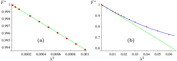
It is important to understand how the optimal time and the corresponding value of fidelity change by increasing the strength of the noise. This should yield information about the robustness of holonomic quantum computation against the detrimental effects of noise. Figure 4(a) shows the behavior of for small noise: the points are the result of a numerical analysis and the continuous line is the fit
| (18) |
yielding . The agrement is excellent and enables one to conclude that fidelity decreases linearly with for . The behavior of for larger values of is displayed in Fig. 4(b). The fit is
| (19) |
with . Observe that is a very large (unphysical) value. The conclusion that fidelity decreases as (for small ) is to be expected from a perturbation expansion of the master equation (17).
Let us now analyze the behavior of the optimal time vs . Figure 5(a) displays the otpimal time vs in the small coupling case. The values of are more affected by errors due to the approximations introduced by the numerical calculations. The optimal time decreases by increasing . The fit yields
| (20) |
with , the value being obtained analytically from Eq. (12). Again, the linear fit is in good agreement with the data and enables one to conclude that the optimal time decreases linearly with for . The behavior of for larger values of is displayed in Fig. 5(b). In this case the fit is
| (21) |
with and .

The behavior of the point is shown in Fig. 6, both for small (a) and larger (b) values of . From Eqs. (18) and (20) one obtains
| (22) |
This is the small coupling situation displayed in Fig. 6(a). Notice that the mean fidelity increases linearly with in this regime. In the presence of noise, optimal quantum gates are less precise and slightly faster than the ideal ones. A further analysis of this dependence for larger values of the noise [using Eqs. (19) and (21)] yields an involved algebraic expression that includes higher order corrections. The behavior is shown in Fig. 6(b). The evolution of the optimal working point is summarized in Fig. 7.


VI Robustness and concluding remarks
In order to shed some light on the robustness of the quantum gate in the neighborhood of the optimal working point it is useful to compare the optimal fidelity with the fidelity obtained in the adiabatic limit . Let us observe that in general, the analysis of decoherence in geometric computation raises a critical issue in connection with adiabatic evolutions, that cannot be too slow, as decoherence would eventually destroy any interference. This inevitably introduces an element of arbitrariness in the following definitions.
We shall evaluate the performance of the optimal (non adiabatic) quantum gate, as compared to its adiabatic limit, throught a “robustness” parameter:
| (23) |
By glancing at Figs. 2 and 3 it is apparent that the adiabatic limit is practically attained already at the third peak, namely for in Eq. (11). We therefore take
| (24) |
The dependence of on is displayed in Fig. 8. Clearly, the (relative) robustness of the optimal gate is larger for larger noise levels. We notice the presence of a linear regime for small coupling.

Although we focused our attention on the particular physical system shown in Fig. 1(a), our conclusions are rather general and are valid for other physically relevant situations. There exist some values of the duration of the evolution for which the fidelity is 1, even though one is far from the adiabatic regime. As already emphasized at the end of Sec. III, these results can be extended to more general loops, yielding optimal times like in Eq. (13).
The presence of these optimal peaks is important for experimental applications: if the total operation time can be tuned to the first peak, one can realize a transformation that is the most robust against noise. Moreover the maximum value of the fidelity exhibits different regimes: for small coupling it decreases linearly with . In general, the gate can be considered robust when compared to the standard adiabatic one. This can be of interest for experimental applications, if one aims at introducing further control. The case of two-qubit gates is not trivial and is at present under investigation.
Acknowledgements.
This work was partly supported by the European Community through the Integrated Project EuroSQIP and by the bilateral Italian Japanese Projects II04C1AF4E on Quantum Information, Computation and Communication of the Italian Ministry of Instruction, University and Research.References
- (1) Geometric phases in physics, A. Shapere and F. Wilczek Eds., (World Scientific, Singapore, 1989).
- (2) A. Bohm, A. Mostafazadeh, H. Koizumi, Q. Niu and J. Zwanziger, The Geometric Phase in Quantum Systems, (Springer, 2003).
- (3) M.A. Nielsen and I.L. Chuang, Quantum Computation and Quantum Information (Cambridge University Press, Cambridge, 2000).
- (4) G. Benenti, G. Casati and G. Strini, Principles of Quantum Computation and Information (World Scientific, Singapore, 2004).
- (5) J. A. Jones, V. Vedral, A. Ekert and G. Castagnoli, Nature, 403, 869 (2000); A. Ekert, M. Ericsson, P. Hayden, H. Inamori, J. A. Jones, D. K. L. Oi and V. Vedral, J. Mod. Opt. 47 2501 (2000).
- (6) P. Zanardi and M. Rasetti, Phys. Lett. A 264, 94 (1999). J. Pachos and P. Zanardi, Int. J. Mod. Phys. B 15, 1257 (2001).
- (7) L. M. Duan, J. I. Cirac and P. Zoller, Science 292, 1695 (2001).
- (8) G. Falci, R. Fazio, G. M. Palma, J. Siewert and V. Vedral, Nature 407, 355 (2000).
- (9) L. Faoro, J. Siewert and R. Fazio, Phys. Rev. Lett. 90, 028301 (2003).
- (10) P. Solinas, P. Zanardi, N. Zanghì and F. Rossi, Phys. Rev. A 67, 062315 (2003).
- (11) D. Giulini, E. Joos, C. Kiefer, J. Kupsch, I.-O. Stamatescu, and H.-D. Zeh, Decoherence and the Appearance of a Classical World in Quantum Theory (Springer, Berlin, 1996).
- (12) P. Solinas, P. Zanardi, and N. Zanghì Phys. Rev. A 70, 042316 (2004).
- (13) I. Fuentes-Guridi, F. Girelli, and E.R. Livine, Phys. Rev. Lett. 94, 020503 (2005).
- (14) G. Florio, P. Facchi, R. Fazio, V. Giovannetti and S. Pascazio, Phys. Rev. A 73, 022327 (2006).
- (15) D. Parodi, M. Sassetti, P. Solinas, P. Zanardi and N. Zanghì, quant-ph/0510056.
- (16) M.S. Sarandy and D.A. Lidar, quant-ph/0507012.
- (17) Y. Aharonov and J. Anandan, Phys. Rev. Lett. 58, 1593 (1987).
- (18) J. Anandan, Phys. Lett. A 133, 171 (1988).
- (19) M. V. Berry, Proc. Roy. Soc. London, Ser. A 392, 45 (1984).
- (20) F. Wilczeck and A. Zee, Phys. Rev. Lett. 52, 2111 (1984); A. Zee, Phys. Rev. A 38, 1 (1988).
- (21) C. W. Gardiner, P. Zoller, Quantum Noise, 2nd Ed., (Springer, Berlin, 2000).
- (22) E. B. Davies and H. Spohn, J. Stat. Phys. 19, 511 (1978).
- (23) P. Facchi, S. Tasaki, S. Pascazio, H. Nakazato, A. Tokuse and D.A. Lidar, Phys. Rev. A 71, 022302 (2005).