Quantum computing with superconductors I: Architectures
Abstract
Josephson junctions have demonstrated enormous potential as qubits for scalable quantum computing architectures. Here we discuss the current approaches for making multi-qubit circuits and performing quantum information processing with them.
1 Introduction
Macroscopic quantum behavior in a Josephson junction (JJ) was first demonstrated in the mid-1980’s by John Clarke’s group at UC Berkeley [17, 9, 18, 7]. These experiments used a superconducting device referred to as a large area, current-biased JJ, which would later become the phase qubit. Beginning in the mid-1990’s the group of James Lukens at SUNY Stony Brook [30, 10] and a collaboration between the Delft University group of Hans Mooij and the MIT group of Terry Orlando [22, 34] demonstrated macroscopic quantum behavior in superconducting loops interrupted by one or more JJs (called superconducting quantum interference devices, or SQUIDS), what would later become flux qubits. And in the late-1990’s the group of Yasunobu Nakamura at NEC in Tsukuba [23, 24] developed the first Cooper-pair box or charge qubit. Many of the earlier experiments were motivated by seminal theoretical work of Caldeira and Leggett [5, 6].
The modern era of superconducting quantum computation began in 2002. That year, the group of Siyuan Han at the University of Kansas and the group of John Martinis, then at NIST Boulder and currently at UC Santa Barbara, independently showed that long-lived quantum states in a current-biassed JJ can be controllably prepared, manipulated, and subsequently measured [40, 19]. This same year, the group of Michel Devoret, then at the CEA in Saclay and currently at Yale University, demonstrated similar quantum control using a Cooper-pair box [35]. These experiments suggest that JJ-based qubits can be used as the building blocks of a solid-state quantum computer, creating a tremendous interest in this intrinsically scalable approach. An impressive list of additional experimental achievements soon followed, including the demonstration of two-qubit quantum logic [37].
In this chapter we will review the current approaches for making multi-qubit systems. For a more detailed discussion of single qubits we refer to the excellent review by Makhlin, Schön, and Shnirman [15]. Also, a recent introductory account of the field has been given by You and Nori [38]. The approach we follow here is to construct circuit models for the basic qubits and coupled-qubit architectures. Many designs have been proposed, but only the simplest have been implemented experimentally to date.
After reviewing in Sec. 2 the basic phase, flux, and charge qubits, we discuss three broad classes of coupling schemes. The simplest class uses fixed linear coupling elements, such as capacitors or inductors, and is discussed in Sec. 3. The principal effect of fixed, weak couplings is to lift degeneracies of the uncoupled qubit pair. However, because such interactions are always present (always turned on), the uncoupled qubit states, which are often used as computational basis states, are not stationary. A variety of approaches have been proposed to overcome this shortcoming. In Sec. 4 we discuss tunable couplings that allow the interactions of Sec. 3 to be tuned, ideally between “on” and “off” values. A related class of dynamic couplings is discussed in Sec. 5, which make use of coupling elements that themselves have active internal degrees of freedom. They act like tunable coupling elements, but also have additional functionality coming from the ability to excite the internal degrees of freedom. Examples of this are resonator-based couplings, which we discuss in some detail.
2 The basic qubits: phase, flux, and charge

The primitive building block for all the qubits is the JJ shown in Fig. 1. The low-energy dynamics of this system is governed by the phase difference between the condensate wave functions or order parameters on the two sides of the insulating barrier. The phase difference is an operator canonically conjugate to the Cooper-pair number difference , according to11 1 We define the momentum to be canonically conjugate to , and In the phase representation, .
| (1) |
The low-energy eigenstates of the JJ can be regarded as probability-amplitude distributions in . As will be explained below, the potential energy of the JJ is manipulated by applying a bias current to the junction, providing an external control of the quantum states , including the qubit energy-level spacing . The crossed box in Fig. 1 represents a ‘‘real” JJ. The cross alone represents a nonlinear element that satisfies the Josephson equations22 2 .
| (2) |
with critical current . The capacitor accounts for junction charging.33 3 This provides a simple mean-field treatment of the inter-condensate electron-electron interaction neglected in the standard tunneling Hamiltonian formalism on which the Josephson equations are based. A single JJ is characterized by two energy scales, the Josephson coupling energy
| (3) |
where is the magnitude of the electron charge, and the Cooper-pair charging energy
| (4) |
with the junction capacitance. For example,
| (5) |
where and are the critical current and junction capacitance in microamperes and picofarads, respectively. In the regimes of interest to quantum computation, and are assumed to be larger than the thermal energy but smaller than the superconducting energy gap which is about in Al. The relative size of and vary, depending on the specific qubit implementation.
2.1 Phase qubit
The basic phase qubit consists of a JJ with an external current bias, and is shown in Fig. 2. The classical Lagrangian for this circuit is
| (6) |
Here
| (7) |
is the effective potential energy of the JJ, shown in Fig. 3. Note that the “mass” in (6) actually has dimensions of The form (6) results from equating the sum of the currents flowing through the capacitor and ideal Josephson element to . The phase qubit implementation uses
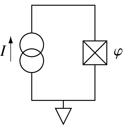
According to the Josephson equations, the classical canonical momentum is proportional to the charge or to the number of Cooper pairs on the capacitor according to . The quantum Hamiltonian can then be written as
| (8) |
where and are operators satisfying (1). Because depends on , which itself depends on time, is generally time-dependent. The low lying stationary states when are shown in Fig. 4. The two lowest eigenstates and are used to make a qubit. is the level spacing and is the height of the barrier.

A useful “spin ” form of the phase qubit Hamiltonian follows by projecting (8) to the qubit subspace. There are two natural ways of doing this. The first is to use the basis of the -dependent eigenstates, in which case
| (9) |
where
| (10) |
The -dependent eigenstates are called instantaneous eigenstates, because is usually changing with time. The time-dependent Schrödinger equation in this basis contains additional terms coming from the time-dependence of the basis states themselves, which can be calculated in closed form in the harmonic limit [11]. These additional terms account for all nonadiabatic effects.
The second spin form uses a basis of eigenstates with a fixed value of bias, . In this case
| (11) |
where
| (12) |
This form is restricted to , but it is very useful for describing rf pulses.

The angle characterizes the width of the eigenstates in . For example, in the -eigenstate basis (and with in the harmonic regime), we have44 4 is the identity matrix.
| (13) |
Here is an effective dipole moment (with dimensions of angle, not length), and .
2.2 Charge qubit
In the charge qubit, the JJ current is provided capacitively, by changing the voltage on a gate, as in Fig. 5. In this case and the small capacitance is achieved by using a Cooper-pair box, which is a nanoscale superconducting island or quantum dot.
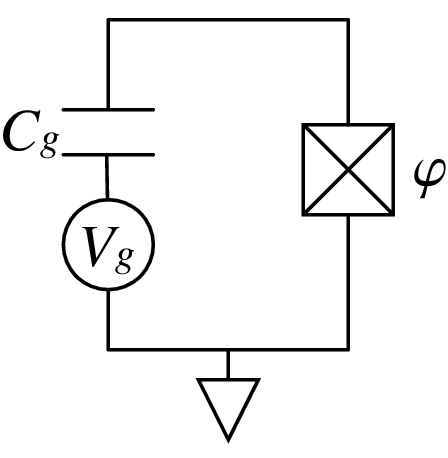
The Lagrangian and Hamiltonian for this system are
| (14) |
and
| (15) |
Here
| (16) |
is the gate charge, the charge qubit’s control variable.
It is most convenient to use the charge representation here, defined by the Cooper-pair number eigenstates satisfying
| (17) |
Because , the term in (15) acts as a Cooper-pair tunneling operator. In the qubit subspace,
| (18) | |||||
| (19) | |||||
| (20) |
The charge qubit Hamiltonian can then be written in spin form in the charge basis as
| (21) |
or in the basis of eigenstates
| (22) |
as
| (23) |
2.3 Flux qubit

The flux qubit uses states of quantized circulation, or magnetic flux, in a SQUID ring. The geometry is illustrated in Fig. 6. The current bias in this case is supplied by the circulating supercurrent. The total magnetic flux can be written as
| (24) |
where is the external contribution and is the self-induced component, with
| (25) |
the circulating current and the self-inductance.55 5 here is not to be confused with the Lagrangian. The relations (24) and (25) determine given , but there is a second condition relating these quantities, namely
| (26) |
This second condition follows from the Meissner effect, which says that the current density in the interior of the ring vanishes, requiring the total vector potential to be proportional to the gradient of the phase of the local order parameter. It is obtained by integrating around the contour in Fig. 6.

The relation (24) then becomes
| (27) |
where
| (28) |
This leads to the Lagrangian and Hamiltonian
| (29) |
and
| (30) |
The ring’s self-inductance has added a quadratic contribution to the potential energy, centered at .
The control variable in the flux qubit is . By choosing
| (31) |
one produces the double-well potential shown in Fig. 7. The condition (31) corresponds of the point of maximum frustration between the two directions of circulating supercurrent. By deviating slightly from the point (31), the energies of the and change, without changing the barrier height that controls the tunneling between the wells.
We can write the flux qubit Hamiltonian in spin form as
| (32) |
where and are parameters that depend on the SQUID geometry and . In the simplest rf SQUID flux qubit discussed here, characterizes the well asymmetry, and is tunable (via ), whereas depends on the barrier height and is fixed by the value of . However, below we will describe a modification that allows the barrier height to be tuned as well.
Hybrid charge-flux qubits have also been demonstrated, and have shown to be successful in reducing decoherence caused by interactions with the environment [35].
3 Fixed linear couplings
By fixed linear couplings we refer to coupling produced by electrically linear elements such as capacitors or inductors that lead to interaction Hamiltonians with fixed coupling strengths. In the cases usually considered, the coupling strengths are also weak, much smaller than the qubit level spacing, and we will assume that here as well. We discuss two prominent examples, capacitively coupled phase and charge qubits. For discussions of the third prominent example, inductively coupled flux qubits, we refer the reader to the literature [22, 25, 15, 20].
3.0.1 Capacitively coupled phase qubits

Capacitively coupled phase qubits have been demonstrated by the University of Maryland group of Fred Wellstood [2] and by the UC Santa Barbara group of John Martinis [21]. The architecture was discussed theoretically by Johnson et al. [13], Blais et al. [4], and Strauch et al. [33].
Referring to Fig. 8, the equations of motion for the two phase variables are66 6
| (33) | |||||
| (34) |
and the Lagrangian is
| (35) |
To find the Hamiltonian, invert the capacitance matrix in
where the are the canonical momenta. This leads to
| (43) |
where
| (44) | |||||
| (45) | |||||
| (46) |
This can be written as
| (47) |
where
| (48) |
The arrow in (48) applies to the further simplified case of identical qubits and weak coupling.
The coupling constant defined in in (48) is inconvenient, however, because the energy scale appearing in (48) is too small. A better definition is
| (49) |
where is the scale introduced in (12).
In the instantaneous basis, the spin form of the momentum operator is
where
| (53) |
Then
| (54) |
In the uncoupled qubit basis , the qubit-qubit interaction in terms of (49) is simply
3.0.2 Capacitively coupled charge qubits

A circuit for capacitively coupled charge qubits is given in Fig. 9. This architecture has been demonstrated by Pashkin et al. [26], and used to perform a CNOT by Yamamoto et al. [37]. This work is currently the most advanced in the field of solid-state quantum information processing. The equations of motion for the two phases are77 7
| (60) | |||||
| (61) |
and the Lagrangian is
| (62) |
Then the Hamiltonian is
| (63) | |||||
where
| (64) | |||||
| (65) | |||||
| (66) |
This can be written as
| (67) |
where
| (68) |
The spin form in the charge basis is
| (69) |
with
| (70) |
When this is a pure Ising interaction.
4 Tunable couplings
By introducing more complicated coupling elements, we can introduce some degree of tunability into the architectures discussed above.
4.0.1 Tunable

A simple way to make the Josephson energy effectively tunable in a circuit is to use a well known quantum interference effect in that occurs in a dc SQUID; see Fig. 10. The tunability of can be understood from two different viewpoints.
The first is to imagine introducing a hole in a current-biased JJ as in the “physical” model of Fig. 10. Tunneling occurs in the up and down direction in each of the left and right arms of the interferometer. Recalling our interpretation of as a Cooper-pair tunneling operator, the two arms of the interferometer result in
| (71) |
Here we have assumed a symmetric interferometer. The first pair of terms corresponds to tunneling (in both the up and down directions) in the left arm, which acquires half of the total Aharonov-Bohm phase ; the right arm has the opposite Aharonov-Bohm phase shift. Then the term in the potential energy of (8) becomes
| (72) |
The effective Josephson energy in (72) can be tuned by varying .
The second way to obtain (72) is to consider the circuit model in Fig. 10, and again assume symmetry (identical JJs). This leads to the coupled equations of motion
| (73) | |||||
| (74) |
The ability to tune is especially useful for inductively coupled flux qubits [15].
4.0.2 Charge qubit register of Makhlin, Schön, and Shnirman

Makhlin, Schön, and Shnirman have proposed coupling charge qubits by placing them in parallel with an inductor, such that the resulting oscillator (the capacitance provided by the JJs) has a frequency much higher than the qubit frequency [14]. The case of two qubits is illustrated in Fig. 11, but the method applies to more than two qubits as well.
The derivation of the circuit Hamiltonian follows methods similar to that used above, and is
| (78) |
The significant feature of the interaction in (78), compared to (70), is that the ’s here can be tuned by using dc SQUIDs. This gives, in principle, a fully tunable interaction between any pair of qubits attached to the same inductor.
4.0.3 Electrostatic transformer of Averin and Bruder

Averin and Bruder [1] considered a related coupled charge qubit circuit, shown in Fig. 12, which we have reorganized to emphasize the similarity to Fig. 11. The Hamiltonian in this case is
| (79) |
and
| (80) |
where
| (81) | |||||
| (82) |
The operator here is a function of the charge qubit variables, but commutes with the transformer degrees of freedom.
As in the register of Makhlin, Schön, and Shnirman, we assume the transformer degrees of freedom are fast compared with the qubit variables, so that the transformer remains in its instantaneous ground state manifold. Then
| (83) |
This finally leads to an effective Hamiltonian
| (84) |
involving charge qubit variables only, where
| (85) | |||||
| (86) |
The discrete second-order derivative , which can be interpreted as a capacitance, can be tuned to zero by varying , providing the desired tunability.
4.1 RF coupling
Finally, we briefly mention an interesting proposal by Rigetti, Blais, and Devoret, to use rf pulses to effectively bring permanently detuned qubits into resonance [29]. This is a very promising approach, but has not yet been demonstrated experimentally.
5 Dynamic couplings: Resonator coupled qubits
Several investigators have proposed the use of resonators [31, 14, 22, 39, 41, 4, 27, 42], superconducting cavities [3, 36], or other types of oscillators [16, 43] to couple JJs together. Although harmonic oscillators are ineffective as computational qubits, because the lowest pair of levels cannot be frequency selected by an external driving field, they are quite desirable as bus qubits or coupling elements. Resonators provide for additional functionality in the coupling, and can be made to have very high factor. Here we will focus on phase qubits coupled by nanomechanical resonators [8, 11, 32, 28].
5.1 Qubit-resonator Hamiltonian

The Hamiltonian that describes the low-energy dynamics of a single large-area, current-biased JJ, coupled to a piezoelectric nanoelectromechanical disk resonator, can be written as [8, 11]
| (87) |
where the and denote particle creation and annihilation operators for the Josephson junction states and denote ladder operators for the phonon states of the resonator’s dilatational (thickness oscillation) mode of frequency , is a coupling constant with dimensions of energy, and . The value of depends on material properties and size of the resonator, and can be designed to achieve a wide range of values. An illustration showing two phase qubits coupled to the same resonator is given in Fig. 13. Interactions between the JJ and resonator may be controlled by changing the JJ current, giving rise to changes in the JJ energy spacing, . For instance, a state can be transferred from the JJ to the resonator by bringing the JJ and resonator in resonance, , and waiting for a specified period.
5.2 Strong coupling and the RWA
For small couplings , the JJ-resonator system may be approximated by the Jaynes-Cummings model; this is usually referred to as the rotating wave approximation (RWA). However, once the coupling becomes comparable to the level spacing, , the RWA breaks down. When the JJ is weakly coupled to the resonator, with below a few percent, gates such as a memory operation (state transfer to and from the resonator) work well, and qubits are stored and retrieved with high fidelity. However, such gates are intrinsically slow. As is increased, making the gate faster, the fidelity becomes very poor, and it becomes necessary to deviate from the RWA protocol. Below, we first discuss an analytical approach to capture the leading corrections to the RWA at intermediate coupling strengths [32]. We then discuss a strong coupling information processing example: a quantum memory register [28].
5.3 Beyond the RWA
For simplicity we will consider only two levels in a single junction. However, all possible phonon-number states are included. The Hamiltonian may then be written as the sum of two terms, . The first term,
| (88) |
is the exactly solvable Jaynes-Cummings Hamiltonian, the eigenfunctions of which are known as dressed states. We will consider the second term,
| (89) |
as a perturbation. The RWA applied to the Hamiltonian amounts to neglecting . Therefore, perturbatively including is equivalent to perturbatively going beyond the RWA.
5.3.1 Dressed states
The eigenstates of , or the dressed states, are labeled by the nonnegative integers and a sign . On resonance, these are
| (90) |
and
| (91) |
Here, the vacuum Rabi frequency on resonance is .
5.3.2 Dressed state propagator
In quantum computing applications one will often be interested in calculating transition amplitudes of the form
| (92) |
where and are arbitrary initial and final states of the uncoupled qubit-resonator system. Expanding and in the dressed-state basis reduces the time-evolution problem to that of calculating the quantity
| (93) |
as well as and . is a propagator in the dressed-state basis, and would be equal to if were absent, that is, in the RWA.
To be specific, we imagine preparing the system at in the state , which corresponds to the qubit in the excited state and the resonator in the ground state . We then calculate the interaction-representation probability amplitude
| (94) |
for the system at a later time to be in the state . Here . Inserting complete sets of the dressed states leads to
| (95) |
and, for ,
| (96) |
So far everything is exact within the model defined in Eq. (87).
To proceed, we expand the dressed-state propagator in a basis of exact eigenstates of , leading to
| (97) |
Here is the energy of stationary state . The propagator is an infinite sum of periodic functions of time. We approximate this quantity by evaluating the and perturbatively in the dressed-state basis.
We test our perturbed dressed-state method for the case of a finite-dimensional single-qubit, five-phonon system. The bias current is chosen to make the system exactly in resonance. The Hamiltonian for this system is diagonalized numerically, and the probability amplitudes are calculated exactly, providing a test of the accuracy of the analytic perturbative solutions. Setting the initial state to be , as assumed previously, we simulate the transfer of a qubit from the Josephson junction to the resonator, by leaving the systems in resonance for half a vacuum Rabi period
In Fig. 14, we plot the probabilities for a relatively strong coupling, . For this coupling strength, the RWA is observed to fail. For example, the RWA predicts a perfect state transfer between the junction and the resonator, and does not exhibit the oscillations present in the exact solution. The dressed state perturbation theory does correctly capture these oscillations.

5.4 Memory operation with strong coupling
Here we study a complete memory operation, where the qubit is stored in the resonator and then transferred back to the JJ, for a large range of JJ-resonator coupling strengths [28]. Also, we show that a dramatic improvement in memory performance can be obtained by a numerical optimization procedure where the resonant interaction times and off-resonant detunings are varied to maximize the overall gate fidelity. This allows larger JJ-resonator couplings to be used, leading to faster gates and therefore more operations carried out within the available coherence time. The results suggest that it should be possible to demonstrate a fast quantum memory using existing superconducting circuits, which would be a significant accomplishment in solid-state quantum computation.
In the upper panel of Fig. 15 we plot the memory fidelity for the qubit state as a function of We actually report the fidelity squared,
| (98) |
which is the probability that the memory device operates correctly. As expected, the fidelity gradually decreases with increasing The lower panel of Fig. 15 gives the gate time as a function of These results suggest that memory fidelities better than 90% can be achieved using phase qubits and resonators with coherence times longer than a few tens of ns.

Acknowledgements.
This work was supported by the NSF under grants DMR-0093217 and CMS-040403.References
- Averin and Bruder (2003) Averin, D. V. and C. Bruder: 2003, ‘Variable electrostatic transformer: Controllable coupling of two charge qubits’. Phys. Rev. Lett. 91, 57003.
- Berkley et al. (2003) Berkley, A. J., H. Xu, R. C. Ramos, M. A. Gubrud, F. W. Strauch, P. R. Johnson, J. R. Anderson, A. J. Dragt, C. J. Lobb, and F. C. Wellstood: 2003, ‘Entangled macroscopic quantum states in two superconducting qubits’. Science 300, 1548–50.
- Blais et al. (2004) Blais, A., R.-S. Huang, A. Wallraff, S. M. Girvin, and R. J. Schoelkopf: 2004, ‘Cavity quantum electrodynamics for superconducting electrical circuits: An architecture for quantum computation’. Phys. Rev. A 69, 62320.
- Blais et al. (2003) Blais, A., A. Massen van den Brink, and A. M. Zagoskin: 2003, ‘Tunable coupling of superconducting qubits’. Phys. Rev. Lett. 90, 127901.
- Caldeira and Leggett (1981) Caldeira, A. O. and A. J. Leggett: 1981, ‘Influence of dissipation on quantum tunneling in macroscopic systems’. Phys. Rev. Lett. 46, 211–4.
- Caldeira and Leggett (1983) Caldeira, A. O. and A. J. Leggett: 1983, ‘Quantum tunneling in a dissipative system’. Ann. Phys. (N.Y.) 149, 374–456.
- Clarke et al. (1988) Clarke, J., A. N. Cleland, M. H. Devoret, D. Esteve, and J. M. Martinis: 1988, ‘Quantum mechanics of a macroscopic variable: The phase difference of a Josephson junction’. Science 239, 992–7.
- Cleland and Geller (2004) Cleland, A. N. and M. R. Geller: 2004, ‘Superconducting qubit storage and entanglement with nanomechanical resonators’. Phys. Rev. Lett. 93, 70501.
- Devoret et al. (1985) Devoret, M. H., J. M. Martinis, and J. Clarke: 1985, ‘Measurements of macroscopic quantum tunneling out of the zero-voltage state of a current-biased Josephson junction’. Phys. Rev. Lett. 55, 1908–11.
- Friedman et al. (2000) Friedman, J. R., V. Patel, W. Chen, S. K. Tolpygo, and J. E. Lukens: 2000, ‘Quantum superpositions of distinct macroscopic states’. Nature (London) 406, 43–6.
- Geller and Cleland (2005) Geller, M. R. and A. N. Cleland: 2005, ‘Superconducting qubits coupled to nanoelectromechanical resonators: An architecture for solid-state quantum information processing’. Phys. Rev. A 71, 32311.
- Geller et al. (2006) Geller, M. R., E. J. Pritchett, A. T. Sornborger, M. Steffen, and J. M. Martinis: 2006, ‘Controlled-NOT logic for Josephson phase qubits’. e-print cond-mat/0000000.
- Johnson et al. (2003) Johnson, P. R., F. W. Strauch, A. J. Dragt, R. C. Ramos, C. J. Lobb, J. R. Anderson, and F. C. Wellstood: 2003, ‘Spectroscopy of capacitively coupled Josephson-junction qubits’. Phys. Rev. B 67, 20509.
- Makhlin et al. (1999) Makhlin, Y., G. Schön, and A. Shnirman: 1999, ‘Josephson-junction qubits with controlled couplings’. Nature (London) 398, 305–7.
- Makhlin et al. (2001) Makhlin, Y., G. Schön, and A. Shnirman: 2001, ‘Quantum-state engineering with Josephson-junction devices’. Rev. Mod. Phys. 73, 357–400.
- Marquardt and Bruder (2001) Marquardt, F. and C. Bruder: 2001, ‘Superposition of two mesoscopically distinct quantum states: Coupling a Cooper-pair box to a large superconducting island’. Phys. Rev. B 63, 54514.
- Martinis et al. (1985) Martinis, J. M., M. H. Devoret, and J. Clarke: 1985, ‘Energy-level quantization in the zero-voltage state of a current-biased Josephson junction’. Phys. Rev. Lett. 55, 1543–6.
- Martinis et al. (1987) Martinis, J. M., M. H. Devoret, and J. Clarke: 1987, ‘Experimental tests for the quantum behavior of a macroscopic degree of freedom: The phase difference across a Josephson junction’. Phys. Rev. B 35, 4682–98.
- Martinis et al. (2002) Martinis, J. M., S. Nam, J. Aumentado, and C. Urbina: 2002, ‘Rabi oscillations in a large Josephson-junction qubit’. Phys. Rev. Lett. 89, 117901.
- Massen van den Brink (2005) Massen van den Brink, A.: 2005, ‘Hamiltonian for coupled flux qubits’. Phys. Rev. B 71, 64503.
- McDermott et al. (2005) McDermott, R., R. W. Simmonds, M. Steffen, K. B. Cooper, K. Cicak, K. D. Osborn, D. P. Oh, S. Pappas, and J. M. Martinis: 2005, ‘Simultaneous state measurement of coupled Josephson phase qubits’. Science 307, 1299–302.
- Mooij et al. (1999) Mooij, J. E., T. P. Orlando, L. S. Levitov, L. Tian, C. H. van der Wal, and S. Lloyd: 1999, ‘Joesphson persistent-current qubit’. Science 285, 1036–9.
- Nakamura et al. (1997) Nakamura, Y., C. D. Chen, and J. S. Tsai: 1997, ‘Spectroscopy of energy-level splitting between two macroscopic quantum states of charge coherently superposed by Josephson coupling’. Phys. Rev. Lett. 79, 2328–31.
- Nakamura et al. (1999) Nakamura, Y., Y. A. Pashkin, and J. S. Tsai: 1999, ‘Coherent control of macroscopic quantum states in a single-Cooper-pair box’. Nature (London) 398, 786–8.
- Orlando et al. (1999) Orlando, T. P., J. E. Mooij, L. Tian, C. H. van der Wal, L. S. Levitov, S. Lloyd, and J. J. Mazo: 1999, ‘Superconducting persistent-current qubit’. Phys. Rev. B 60, 15398–413.
- Pashkin et al. (2003) Pashkin, Y. A., T. Yamamoto, O. Astafiev, Y. Nakamura, D. V. Averin, and J. S. Tsai: 2003, ‘Quantum oscillations in two coupled charge qubits’. Nature (London) 421, 823–6.
- Plastina and Falci (2003) Plastina, F. and G. Falci: 2003, ‘Communicating Josephson qubits’. Phys. Rev. B 67, 224514.
- Pritchett and Geller (2005) Pritchett, E. J. and M. R. Geller: 2005, ‘Quantum memory for superconducting qubits’. Phys. Rev. A 72, 10301.
- Rigetti et al. (2005) Rigetti, C., A. Blais, and M. H. Devoret: 2005, ‘Protocol for universal gates in optimally biased superconducting qubits’. Phys. Rev. Lett. 94, 240502.
- Rouse et al. (1995) Rouse, R., S. Han, and J. E. Lukens: 1995, ‘Observation of resonant tunneling between macroscopically discinct quantum levels’. Phys. Rev. Lett. 75, 1614–7.
- Shnirman et al. (1997) Shnirman, A., G. Schön, and Z. Hermon: 1997, ‘Quantum manipulations of small Josephson junctions’. Phys. Rev. Lett. 79, 2371–4.
- Sornborger et al. (2004) Sornborger, A. T., A. N. Cleland, and M. R. Geller: 2004, ‘Superconducting phase qubit coupled to a nanomechanical resonator: Beyond the rotating-wave approximation’. Phys. Rev. A 70, 52315.
- Strauch et al. (2003) Strauch, F. W., P. R. Johnson, A. J. Dragt, C. J. Lobb, J. R. Anderson, and F. C. Wellstood: 2003, ‘Quantum logic gates for coupled superconducting phase qubits’. Phys. Rev. Lett. 91, 167005.
- van der Wal et al. (2000) van der Wal, C. H., A. C. J. ter Haar, F. K. Wilhelm, R. N. Schouten, C. J. P. M. Harmans, T. P. Orlando, S. Lloyd, and J. E. Mooij: 2000, ‘Quantum superpositions of macroscopic persistent current’. Science 290, 773–7.
- Vion et al. (2002) Vion, V., A. Aassime, A. Cottet, P. Joyez, H. Pothier, C. Urbina, D. Esteve, and M. H. Devoret: 2002, ‘Manipulating the quantum state of an electrical circuit’. Science 296, 886–9.
- Wallraff et al. (2004) Wallraff, A., D. I. Schuster, A. Blais, L. Frunzio, R.-S. Huang, J. Majer, S. Kumar, S. M. Girvin, and R. J. Schoelkopf: 2004, ‘Strong coupling of a single photon to a superconducting qubit using circuit quantum electrodynamics’. Nature (London) 431, 162–7.
- Yamamoto et al. (2003) Yamamoto, T., Y. A. Pashkin, O. Astafiev, Y. Nakamura, and J. S. Tsai: 2003, ‘Demonstration of conditional gate operations using superconducting charge qubits’. Nature (London) 425, 941–4.
- You and Nori (2005) You, J. Q. and F. Nori: 2005, ‘Superconducting circuits and quantum information’. Physics Today, November 2005. p. 42.
- You et al. (2002) You, J. Q., J. S. Tsai, and F. Nori: 2002, ‘Scalable quantum computing with Josephson charge qubits’. Phys. Rev. Lett. 89, 197902.
- Yu et al. (2002) Yu, Y., S. Han, X. Chu, S.-I. Chu, and Z. Wang: 2002, ‘Coherent temporal oscillations of macroscopic quantum states in a Josephson junction’. Science 296, 889–92.
- Yukon (2002) Yukon, S. P.: 2002, ‘A multi-Josephson junction qubit’. Physica C 368, 320–3.
- Zhou et al. (2004) Zhou, X., M. Wulf, Z. Zhou, G. Guo, and M. J. Feldman: 2004, ‘Dispersive manipulation of paired superconducting qubits’. Phys. Rev. A 69, 30301.
- Zhu et al. (2003) Zhu, S.-L., Z. D. Wang, and K. Yang: 2003, ‘Quantum-information processing using Josephson junctions coupled through cavities’. Phys. Rev. A 68, 34303.