Entanglement Distribution Revealed by Macroscopic Observations

Observation of quantum entanglement between increasingly larger objects is one of the most promising avenues of experimental quantum physics. Eventually, all these developments might lead to a full understanding of the simultaneous coexistence of a macroscopic classical world and an underlying quantum realm. Macroscopic samples typically contain $N\sim 10^{23}$ particles. Because the system’s Hilbert space grows exponentially with the number of constituent particles, a complete microscopic picture of entanglement in large systems seems to be in general intractable. The question arises: What can we learn about entanglement between constituent particles of macroscopic samples, if only limited experimentally accessible knowledge about the samples is available?

There is a strong motivation in addressing this question because of recent experimental progress in creating and manipulating entangled states of increasing complexity, such as spin-squeezed states of two atomic ensembles Polzik. In such experiments one typically measures only expectation values of collective operators of two separated samples. It is known that the two samples of spins can be characterized as either entangled or separable by measuring collective spin operators Sorensen. Furthermore, such measurements are shown to be sufficient to determine entanglement measures of Gaussian states Molmer and of a pair of particles that are extracted from a totally symmetric spin state (invariant under exchange of particles) WangMolmer. It appears that collective operators cannot be used to fully characterize entanglement in composite systems without strong requirements on the symmetry of the state.

Here we present a general and practical method for entanglement detection between two samples of spins. It solely employs collective spin properties of the samples and works irrespective of the number of spin particles constituting the samples and with no assumption about the symmetry or mixedness of the state. The method is based on an entanglement measure which is a tight lower bound for average entanglement between all pairs of spins belonging to the two samples. This measure is equal to the average entanglement for a certain class of systems which need not be totally symmetric. We generalize the method to obtain the entanglement measure between $M$ separated spin samples based on collective measurements. The results apply for any entanglement monotone that is a convex measure on the set of density matrices (e.g., concurrence Wootters, negativity Zycz1998, three-way tangle Coffman).

Consider two separated ensembles $A$ and $B$ of spin-$\frac{1}{2}$ particles (figure 1). Each of them contains a large number $n$ of spins. Because of the large dimensions ($d=2^{n}$) of the samples’ Hilbert spaces, the structure of entanglement between the two samples is considerably more complex than between two single spins. While there are experimentally viable methods for detecting entanglement, they still require a large number of parameters to be determined (proportional to $d^{2}$ Horodecki). The problem simplifies in situations in which each of the ensembles of $n$ spins can be treated as one large (total) spin of length $n/2$. This means that, within the ensembles, the individual spin-$\frac{1}{2}$ particles form symmetrized states (Dicke states). Though this reduces the dimension of the Hilbert space of $A$ ($B$) to $d=n+1$, entanglement determination is still demanding for large $n$ both experimentally and theoretically: analytical solutions exist only for pure states in general and for mixed states only for small $n$ Schliemann.

In this paper, we give a method to detect entanglement between large spin samples by measuring only a small number of collective spin properties (sample spin components and their correlations), which is independent of the sample size $n$. The collective spin operators are

The index $i$ denotes the spatial component of the spins: $i\in\{1\!\equiv\!x,2\!\equiv\!y,3\!\equiv\!z\}$. The Pauli matrix of the spin at site $\alpha\in A$ is given by $\hat{\sigma}_{i}^{(\alpha)}$, and analogously for a spin $\beta$ from subsystem $B$. Note that the collective operators satisfy the usual commutation relations $[\hat{S}_{i}^{A},\hat{S}_{j}^{A}]=\;$i$\,\hbar\,\varepsilon_{ijk}\,\hat{S}_{k}^{A}$, since $[\hat{\sigma}_{i}^{(\alpha)},\hat{\sigma}_{j}^{(\alpha^{\prime})}]=2\,$i$\,\varepsilon_{ijk}\,\hat{\sigma}_{k}^{(\alpha)}\,\delta_{\alpha\alpha^{\prime}}$.

The spin expectation values and correlations are

and analogously for $S_{i}^{B}\equiv\frac{\hbar}{2}\,{\sum\nolimits_{\beta\in B}}\,g_{i}(\beta)$, where $S_{i}^{A},S_{i}^{B}\!\in\![-\frac{n\hbar}{2},\frac{n\hbar}{2}]$, $T_{ij}^{AB}\!\in\![-\frac{n^{2}\hbar^{2}}{4},\frac{n^{2}\hbar^{2}}{4}]$. These are only 15 numbers. Here $g_{i}(\alpha)$, $g_{i}(\beta)$ and $h_{ij}(\alpha,\beta)$ are the (dimensionless) expectation values and pair correlations of two single spins ($\alpha,\beta$) to which it is assumed there is no experimental access: $g_{i}(\alpha)\equiv\left\langle\!\right.\hat{\sigma}_{i}^{(\alpha)}\left.\!\right\rangle_{\hat{\rho}_{\alpha\beta}}$, $h_{ij}(\alpha,\beta)\equiv\left\langle\!\right.\hat{\sigma}_{i}^{(\alpha)}\hat{\sigma}_{j}^{(\beta)}\left.\!\right\rangle_{\hat{\rho}_{\alpha\beta}}$. They are obtained from the actual $4\!\times\!4$ density matrix

where $\mathbf{1}^{(\alpha)}$ is the $2\!\times\!2$ identity matrix in the Hilbert space of spin $\alpha$.

Out of the experimentally accessible quantities (2) and (3) we will construct a $4\!\times\!4$ density matrix of two virtual qubits which describes the collective properties of the two spin sets. Its a priori justification is (i) that a general treatment of the problem between two large samples of spins is intractable because of the high dimensionality, and (ii) that we have a fully developed theory of entanglement for two-qubit systems. Therefore, this approach is a natural (and successful) way to say something at all about the entanglement between two spin systems if only collective observables are measured.

We first introduce the normalized (dimensionless) average subsystem expectation values (magnetization per particle) and correlations:

where $s_{i}^{a},t_{ij}^{ab}\in[-1,1]$. These are the coefficients of the virtual density matrix:

with $a$ denoting the first and $b$ the second virtual collective qubit, associated with subsystems $A$ and $B$, respectively. Here, $\mathbf{1}^{a}$, $\mathbf{1}^{b}$, $\hat{\sigma}_{k}^{a}$ and $\hat{\sigma}_{l}^{b}$ are $2\!\times\!2$ identity and Pauli matrices for the collective qubits $a$ and $b$.

The question is whether the density matrix (7) is positive semi-definite, i.e., whether it is a physical state of two qubits. The answer is affirmative and the proof follows from consideration of an equal-weight statistical mixture of one qubit pair which can be in any of the $n^{2}$ states $\hat{\rho}_{\alpha\beta}$. The density matrix of this mixture is the mixture of density matrices of all possible pairs ($\alpha,\beta$): $\hat{\rho}_{\text{mix}}=\frac{1}{n^{2}}\,{\sum\nolimits_{\alpha,\beta}}\,\hat{\rho}_{\alpha\beta}$. It can easily be seen that $\hat{\rho}_{\text{mix}}$ is equal to $\hat{\rho}_{ab}$ as both are uniquely determined by the same expectations and correlations: $\langle\hat{\sigma}_{i}^{(\alpha)}\rangle_{\hat{\rho}_{\text{mix}}}=\langle\hat{\sigma}_{i}^{a}\rangle_{\hat{\rho}_{ab}}=s_{i}^{a}=\frac{2}{n\hbar}\,S_{i}^{A}$ and $\langle\hat{\sigma}_{i}^{(\alpha)}\hat{\sigma}_{j}^{(\beta)}\rangle_{\hat{\rho}_{\text{mix}}}=\langle\hat{\sigma}_{i}^{a}\hat{\sigma}_{j}^{b}\rangle_{\hat{\rho}_{ab}}=t_{ij}^{ab}=\frac{4}{n^{2}\hbar^{2}}\,T_{ij}^{AB}$. Thus, $\hat{\rho}_{ab}$ is a density matrix. Note that without the normalizations as given in (5) and (6), the method would not work.

Encapsulated in the following two propositions, we relate the entanglement properties of the virtual qubits to those of the spin samples.

Proposition 1. For any entanglement measure $E$ that is convex on the set of density matrices the entanglement of the virtual density matrix $E_{ab}\equiv E(\hat{\rho}_{ab})$ is a lower bound for the average entanglement between all pairs $\bar{E}_{\alpha\beta}\equiv\tfrac{1}{n^{2}}\,\sum\nolimits_{\alpha,\beta}\,E(\hat{\rho}_{\alpha\beta})$. This is an immediate consequence of the convexity of $E$: $E_{ab}=E(\tfrac{1}{n^{2}}\,{\sum\nolimits_{\alpha,\beta}}\,\hat{\rho}_{\alpha\beta})\leq\tfrac{1}{n^{2}}\,{\sum\nolimits_{\alpha,\beta}}\,E(\hat{\rho}_{\alpha\beta})$.

Remarks: First, the result holds for entanglement measures that are convex. In certain cases this is directly implied by the definition of the entanglement measure for mixed states, which involves a convex roof $E(\hat{\rho})\equiv\text{min}_{p_{i},\psi_{i}}\sum_{i}p_{i}\,E(|\psi_{i}\rangle\langle\psi_{i}|)$, where the minimization is taken over those probabilities $\{p_{i}\}$ and pure states $|\psi_{i}\rangle$ that realize the density matrix $\hat{\rho}=\sum_{i}p_{i}|\psi_{i}\rangle\langle\psi_{i}|$ and $E(|\psi_{i}\rangle\langle\psi_{i}|)$ is the entanglement measure of the pure state $|\psi_{i}\rangle$. Second, the proposition implies that if $E_{ab}\!>\!0$ then at least for one pair we must have $E(\hat{\rho}_{\alpha\beta})\!>\!0$. Thus, a non-zero value of $E_{ab}$ is a sufficient condition for entanglement between the two samples $A$ and $B$. Third, the maximal pairwise concurrence Wootters for symmetric states is found to be $2/n$ and is achieved for the W-state Koachi. It is conjectured that this remains valid also when the symmetry constraint is removed. This suggests $E_{ab}\leq\bar{E}_{\alpha\beta}\leq 2/n$, if concurrence is used as an entanglement measure. The existence of this upper bound can be seen as a consequence of the monogamy of entanglement.

We refer to $E_{ab}$ as pairwise collective entanglement as it is determined solely by the expectation and correlation values of the collective spin observables. The question arises: Under what conditions is $E_{ab}$ equal to the average entanglement $\bar{E}_{\alpha\beta}$? Identifying systems for which the equality holds, would allow feasible experimental determination of the entanglement distribution in large samples by observation of their macroscopic properties only. It can easily be seen that, if the state is symmetric under exchange of particles within each of the samples, one has $E_{ab}=\bar{E}_{\alpha\beta}=E(\hat{\rho}_{\alpha\beta})$ for every pair of particles $(\alpha,\beta)$. In what follows, we identify an important class of systems for which $E_{ab}\!=\!\bar{E}_{\alpha\beta}$ though the corresponding states need not be symmetric under exchange of particles.

Proposition 2. Consider a system (i) with $g_{z}(\alpha)=g_{z}^{A}$ for all $\alpha\in A$ and $g_{z}(\beta)=g_{z}^{B}$ for all $\beta\in B$ (translational invariance within the subsystems), (ii) with $h_{xx}(\alpha,\beta)=\varepsilon\,h_{yy}(\alpha,\beta)$ with $\varepsilon=\;$const$\;=+1$ or $-1$ (all pairs are in absolute value equally correlated in the $x$ and $y$-direction, where this correlation may be different in size for different pairs), (iii) with constant sign of the $z$-correlations, i.e., sgn$[h_{zz}(\alpha,\beta)]=-\varepsilon$ for all $(\alpha,\beta)$, and (iv) where all the remaining expectation values and correlations ($g_{x}$, $g_{y}$, $h_{ij}$ with $i\neq j$) are zero. Non-vanishing average entanglement $\bar{E}_{\alpha\beta}$ as measured by the negativity Zycz1998 is equal to the pairwise collective entanglement $E_{ab}$, if and only if the correlation functions $h_{xx}(\alpha,\beta)$ and $h_{yy}(\alpha,\beta)$ are each constant for all pairs and all pairs have a non-positive eigenvalue of their partial transposed density matrix.

The negativity Zycz1998 of a density matrix $\hat{\rho}$ is defined as $E(\hat{\rho})\equiv(\text{Tr}|\hat{\rho}^{\text{pT}}|-1)/2$, where $\text{Tr}|\hat{\rho}^{\text{pT}}|$ stands for the trace norm of the partially transposed density matrix $\hat{\rho}^{\text{pT}}$. Hence the negativity is equal to the modulus of the sum of the negative eigenvalues of $\rho^{\text{pT}}$.

It is important to stress that proposition 2 holds also for states that do not need to be totally symmetric, i.e., the $h_{zz}(\alpha,\beta)$ may be different for different pairs of particles. In general, under the above symmetry, the state of the virtual qubit pair is of the form

where $u_{\pm\pm\pm}\equiv\frac{1}{4}\,(1\pm s_{z}^{A}\pm s_{z}^{B}\pm t_{zz}^{ab})$, $v_{\pm}\equiv\frac{1}{4}\,t_{xx}^{ab}\,(1\pm\varepsilon)$. The state of an arbitrary pair $(\alpha,\beta)$ of particles has a similar structure. For example, the state of an arbitrary pair of particles extracted from a spin chain with $xxz$ Heisenberg interaction has such a form. The proof of proposition 2 is given in the appendix.

We illustrate the method with some explicit examples.

1. Dicke states. We consider the Dicke state (generalized W-state)

with $N\geq 2$ spins, $k$ excitations $|1\rangle$ and $N-k$ non-excited spins $|0\rangle$, where $0\leq k\leq N$. $\hat{P}_{S}$ is the symmetrization operator. Within the system we consider two subsystems $A$ and $B$ each of size $n$. Because of the total symmetry of the state one has $E_{ab}=\bar{E}_{\alpha\beta}=E(\hat{\rho}_{\alpha\beta})$ for any size $n$. Only for the cases where just a single spin ($k=0$) or all spins are excited ($k=N$), there is no entanglement between two arbitrary pairs or arbitrary sized blocks, respectively Vedr2004. The global maximum of the entanglement $E_{ab}$, measured by the negativity, is reached for $k=\frac{N}{2}$ and its value is $E_{ab}^{\text{max}}=\frac{1}{2}\,\frac{1}{N-1}$, for all $n$. It vanishes only in the limit $N\rightarrow\infty$.

2. Generalized singlet states. The two subsystems $A$ and $B$, each forming a spin $s=\frac{n}{2}$, are in a generalized singlet state:

where $\left|m\right\rangle=\left|2\,s;s+m\right\rangle$ denotes the eigenstates of the spin operator’s $z$-component. The collective two-qubit coefficients are $t_{ii}^{ab}=-\frac{n+2}{3n}$ and the $s_{i}^{a,b}$ and $t_{ij}^{ab}$ with $i\neq j$ are all zero. The collective entanglement (negativity) is $E_{ab}=\frac{1}{2n}=\frac{1}{4s}$ which is non-zero for all sizes $n$ of the subsystems and vanishes only in the limit $n\rightarrow\infty$.

3. Generalized singlet state with an admixture of non-symmetric correlations. Consider the state

with $p\in[0,1]$. This is a mixture of the generalized singlet state (10) and $n$ perfectly $z$-correlated pairs ($\alpha,\beta\!=\!\alpha$). This state is not symmetric under particle exchange in the $zz$-correlations. The expectation values $s_{i}^{a,b}$ and correlations $t_{ij}^{ab}$ with $i\neq j$ remain zero. The correlations $t_{xx}=t_{yy}$ are reduced by a factor $p$ compared to those of the state (10). The correlations in $z$-direction, however, are modified and read $t_{zz}^{ab}=-p\,\frac{n-1}{3n}-\frac{1}{n}$. Therefore, there is a critical number of particles $n_{c}\equiv\left\lceil\!\right.\frac{1+p}{1-p}\left.\!\right\rceil$ beyond which there is no collective pairwise entanglement. Only for $n<n_{c}$ we have $E_{ab}=\frac{1}{4}\frac{1+p-n\,(1-p)}{n}>0$. Note that (11) is in accordance with proposition 2 (appendix) and thus $E_{ab}=\bar{E}_{\alpha\beta}$. Figure 2 shows $E_{ab}$ as a function of the spin length $s=\frac{n}{2}$ and the mixing parameter $p$. $E_{ab}$ is non-zero in regions where $p>\frac{2s-1}{2s+1}$ and decreases inversely proportionally to $s$.

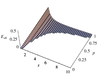
Our method can be generalized straightforwardly to define multi-partite entanglement of $M$ collective spins belonging to $M$ separated samples $A_{1},...,A_{M}$, each containing a large number of spins $n$. Any convex multi-partite entanglement measure (e.g., $M$-way tangle) which is applied to the corresponding collective matrix of the $M$ virtual qubits gives a lower bound for the average multi-partite entanglement, obeying the usual constraints for entanglement sharing such as the Coffman–Kundu–Wootters inequality Coffman.

Importantly, in the examples considered above our entanglement measure scales at most with $1/n$ and vanishes in the limit of infinitely large subsystem sizes $n$. This is a generic property that follows from the commutation relation for normalized spins in this limit. Taking $\hat{s}_{i}\equiv\frac{1}{n}\,\hat{S}_{i}=\frac{\hbar}{2n}\sum_{\alpha}\hat{\sigma}_{i}^{(\alpha)}$ one obtains $\lim_{n\rightarrow\infty}[\hat{s}_{x},\hat{s}_{y}]=\lim_{n\rightarrow\infty}\,$i$\,\frac{\hbar}{2n}\,\hat{s}_{z}=0$. This is sometimes interpreted as suggesting that averaged collective observables, like the magnetization per particle, represent ”macroscopic” or classical-like, properties of samples. Note, however, that for any $n$ there are $n^{2}$ pairs between the subsystems so that the number of pairs multiplied by the pairwise collective entanglement can scale with $n$, showing the existence of entanglement for arbitrarily large $n$.

Conclusion. In a recent work it was shown that macroscopic properties such as magnetic susceptibility can reveal entanglement within macroscopic samples Wiesniak. The present work can be viewed as in a way complementary as it demonstrates that macroscopic properties (collective spin properties and their correlations) can reveal the entanglement distribution between two or more macroscopic samples. On the fundamental side, our method demonstrates that there is no reason in principle why purely quantum correlations could not have an effect on the global properties of objects. On the practical side, it enables us to characterize the structure of entanglement in large spin systems by performing only a few feasible measurements of their collective properties, independent of the symmetry and mixedness of the state.

This work was supported by the Austrian Science Foundation, Proj. SFB (No. 1506), the Europ. Commission, Proj. QAP (No. 015846), and the British Council in Austria.

Appendix. Proof of proposition 2. Depending on the sign $\varepsilon$ of the $zz$-correlations, only one eigenvalue of $\hat{\rho}_{\alpha\beta}^{\text{pT}}$ and $\hat{\rho}_{ab}^{\text{pT}}$, respectively, can be negative:

The corresponding negativities are given by $E_{\alpha\beta}=|\!\min(0,\mu_{\alpha\beta})|$ and $E_{ab}=|\!\min(0,\nu_{ab})|$. One can express $\nu_{ab}$ as given by

where $\bar{\mu}\equiv\frac{1}{n^{2}}\,{\sum\nolimits_{\alpha,\beta}}\,\mu_{\alpha\beta}$ and $\Delta\equiv\frac{1}{4n^{2}}\,{\sum\nolimits_{\alpha,\beta}}[(g_{z}^{A}+\varepsilon\,g_{z}^{B})^{2}+4\,h_{xx}^{2}(\alpha,\beta)]^{1/2}-\frac{1}{4}[(s_{z}^{a}+\varepsilon\,s_{z}^{b})^{2}+4\,(t_{xx}^{ab})^{2}]^{1/2}$. The quantity $\Delta$ is the difference between the entanglement measures $\bar{E}_{\alpha\beta}$ and $E_{ab}$, i.e., $E_{ab}=\bar{E}_{\alpha\beta}-\Delta$, for the case that $\nu_{ab}\leq 0$ and $\bar{E}_{\alpha\beta}\equiv\tfrac{1}{n^{2}}\,{\sum\nolimits_{\alpha,\beta}}\,|\!\min(0,\mu_{\alpha\beta})|=|\!\min(0,\bar{\mu})|$. This is true, if and only if $\mu_{\alpha\beta}\leq 0$ for all ($\alpha,\beta$), i.e., all pairs are either entangled or have eigenvalue zero. According to proposition 1, $\Delta$ is non-negative, i.e.,

Here we abbreviated $c\equiv g_{z}^{A}+\varepsilon\,g_{z}^{B}=s_{z}^{a}+\varepsilon\,s_{z}^{b}$, where the latter equal sign is due to (5). Inequality (14) becomes an equality, i.e., $\Delta=0$, if and only if $h_{xx}(\alpha,\beta)$ is the same for all pairs $(\alpha,\beta)$ such that $t_{xx}^{ab}=h_{xx}$. Therefore, the pairwise collective entanglement $E_{ab}$ equals the average entanglement $\bar{E}_{\alpha\beta}$, if and only if for all individual pairs $\mu_{\alpha\beta}\leq 0$ and $h_{xx}(\alpha,\beta)=\varepsilon\,h_{yy}(\alpha,\beta)=\;$const for all pairs. $\square$

References

- (1) B. Julsgaard, A. Kozhekin, and E. S. Polzik, Nature (London) 413, 400 (2001).
- (2) A. Sørensen, L.-M. Duan, J. Cirac, and P. Zoller, Nature (London) 409, 63 (2001).
- (3) J. Sherson and K. Mølmer, Phys. Rev. A 71, 033813 (2005).
- (4) X.Wang and K. Mølmer, Eur. Phys. J. D 18, 385 (2002).
- (5) S. Hill and W. K. Wootters, Phys. Rev. Lett. 78, 5022 (1997).
- (6) K. Życzkowski, P. Horodecki, A. Sanpera, and M. Lewenstein, Phys. Rev. A 58, 883 (1998); G. Vidal and R. F. Werner, Phys. Rev. A 65, 032314 (2002).
- (7) V. Coffman, J. Kundu, and W. K. Wootters, Phys. Rev. A 61, 052306 (2000).
- (8) P. Horodecki and A. Ekert, Phys. Rev. Lett. 89, 127902 (2002).
- (9) J. Schliemann, Phys. Rev. A 72, 012307 (2005).
- (10) M. Koashi, V. Bužek, and N. Imoto, Phys. Rev. A 62, 050302(R) (2000).
- (11) V. Vedral, New J. Phys. 6, 102 (2004).
- (12) M. Wiesniak, V. Vedral, and Č. Brukner, New J. Phys. 7, 258 (2005); Č. Brukner, V. Vedral, and A. Zeilinger, Phys. Rev. A 73, 012110 (2006).