One-dimensional models of disordered quantum wires: general
formalism
Alberto Rodríguez 11
1
email:argon@usal.es
Física Teórica. Departamento de Física Fundamental. Universidad
de Salamanca. 37008 Salamanca. Spain
In this work we describe, compile and generalize a set of tools that can be used to analyse the electronic
properties (distribution of states, nature of states, …) of
one-dimensional disordered compositions of potentials. In particular, we derive an ensemble of universal functional equations
which characterize the thermodynamic limit of all one-dimensional models
and which only depend formally on the distributions that define the
disorder. The equations are useful to obtain relevant quantities of the system such as density of states or
localization length in the thermodynamic limit.
Introduction
The pioneering work of Anderson [1] changed completely the understanding of the properties of disordered systems and meant the opening of a research field which is of primary importance nowadays. The physics of disordered systems is currently a significant part of condensed matter physics and it has been the subject of an intense research activity specially during the last ten years. Electronic localization due to disorder is a key element to understand different physical phenomena such as the Quantum Hall Effect or the suppression of conductivity in amorphous matter. In the last years the effect of the presence of statistical correlations in disordered systems has been analysed [2, 3, 4, 5, 6, 7] and the conclusions regarding the appearance of extended states in the spectrum have been experimentally confirmed for the case of short-range correlations [8] as well as for long-range correlations [9, 10]. Scaling theory and Universality of the distributions of transport-related quantities characterizing disordered systems are subjects which are still evolving nowadays: the conditions for the validity of single parameter scaling (SPS) have been recently reformulated [11, 12] and it has been found that different scaling regimes appear when disorder is correlated [13]. The presence of disorder is of key importance for the characterization of low-dimensional structures, such as one-dimensional quantum wires, since it plays a key role in the transport processes and it can strongly alter the electronic properties of the system. Unlike the case of ordered matter, for disordered systems there is a lack of a general theory describing in a compact form their physical properties. Nevertheless a large ensemble of different techniques exists that can be used to unravel some features of this kind of structures. Our fundamental premise to study the electronic properties of one-dimensional disordered systems is to consider non-interacting spinless carriers within the independent particle approximation, that is the Hamiltonian of the system only includes the potential of a linear array of different atomic units . Also our approach focuses on the characterization of the static transport properties of these structures. Within this framework, the aim of this work is to describe, compile and generalize a set of tools that can be used for all one-dimensional systems in order to analyse their electronic properties (distribution of states, nature of states, …). In particular, we derive an ensemble of universal functional equations which characterize the thermodynamic limit of all one-dimensional models (within the approximations made above) and that are useful to obtain relevant quantities of the system such as density of states or localization length in that limit. Therefore a great part of our efforts are aimed at contributing to the growth of a general methodology that can be applied to all potential models in one-dimension. Let us also mention that the formalism here contained has already been used by the author and co-workers to describe successfully a large variety of one-dimensional disordered models [35, 36, 37, 38, 39]. However a complete and general derivation of the theoretical formalism is still lacking; the present work comes to fill this gap.
The work is organized as follows. In section 1 we make a thorough description of the continuous transmission matrix formalism and its applicability to finite-range as well as continuous potentials. Detailed analysis and calculations completing this section are contained in appendix A. The canonical equation and its derivation from the transmission matrix is treated in section 2. In section 3 the discrete transmission matrix formalism is briefly commented. The reliable parameters that can be used to characterize electronic localization are described in section 4, where we particularly focus on the Lyapunov exponents, whose analysis is completed in appendix B. The procedure to calculate the distribution of states for the disordered chain is explained and generalize in section 5 and appendix C, to proceed subsequently with the construction of the functional equation formalism which is contained in section 6 and constitutes the main body of the work. The expressions of DOS and localization length in the thermodynamic limit in terms of the solutions of the functional equations are rigorously obtained. The applicability of the formalism developed is illustrated studying the one-dimensional tight-binding model.
1 Continuous transmission matrix formalism
The time-independent scattering process of a one-dimensional potential can be described using the well-known continuous transfer matrix method,
| (1) |
where , (, ), mean the amplitudes of the asymptotic travelling plane waves , , at the left (right) side of the potential. The peculiarities of the transmission matrix and its elements depend on the nature of the potential. A detailed analysis on this subject can be found in appendix A. As a summary let us say that for real potentials belongs to the group and that the property holds for all kind of potentials whether they are real or complex.
The transmission and reflection scattering amplitudes of the potential read
| (2) |
where the superscripts , , stand for left and right incidence. The insensitivity of the transmission amplitude to the incidence direction is a universal property. In general the reflection amplitudes will differ, although for real potentials and complex ones with parity symmetry [14].
Obtaining the transmission matrix is specially easy for discontinuous short-range potentials such as deltas or square well/barriers, for which the asymptotic limit is not necessary to satisfy equation (1). In these cases the effect of a composition of different potential units can be considered through the product of their transmission matrices,
| (3) |
therefore obtaining analytically or numerically the exact scattering probabilities of the whole structure. This formalism can also be used to obtain the bound states from the poles of the complex transmission amplitude. An intuitive and general interpretation of the composition procedure can be given in the following form. Let us consider two finite range potentials , , characterized by the amplitudes , , , , , , and joined at a certain point. Then, the scattering amplitudes of the composite potential can be obtained by considering the coherent sum of all the multiple reflection processes that might occur at the connection region [15],
| (4a) | ||||
| (4b) | ||||
| (4c) | ||||
Replacing the scattering amplitudes with the elements of the corresponding transmission matrices , , one can trivially check that in fact the latter formulae are the equations of the matrix product . Thus, the composition rules given by (4) are not restricted to the convergence interval of the series . They provide an explicit relation of the global scattering amplitudes in terms of the individual former ones and can be easily used recurrently for numerical purposes.
For continuous potentials the calculation of the transfer matrix is more complex. After solving the Schrödinger equation for positive energies, one has to take the limits to recover the free particle states and identify the matrix elements. Hence equation (1) is strictly satisfied only asymptotically. However depending on the decay of the potential one could neglect its effects outside a certain length range.

If the asymptotic transmission matrix of the potential in figure 1 is known, then the matrix for the cut-off potential contained between the dashed lines can be written as (see appendix A)
| (5) |
The cut-off matrix is the same as the asymptotic one plus an extra phase term in the diagonal elements that accounts for the total distance during which the particle feels the effect of the potential, and also an extra phase term in the off-diagonal elements measuring the asymmetry of the cut-off . Doing such approximation one gets matrices suitable to be composed in linear arrays.
2 The canonical equation
As stated in the introduction we are treating one-dimensional atomic wires within the independent particle approximation. The electron-electron interaction is not considered and also the carriers are supposed to be spinless. Then, the Hamiltonian of the system only includes the potential of a linear array of different atomic units. From the solutions of the one-particle Schrödinger equation it is always possible to derive an expression with the following canonical form22 2 The meaning of the coefficients appearing in the canonical equation depends on the particular Hamiltonian. For a tight-binding model they have a straightforward interpretation in terms of the on-site energies and the transfer integrals, thus the equation is usually written in the form . For other models that comparison may not be so clear, so we keep a more general expression. [16, 4]
| (6) |
where means the amplitude of the electronic state at the th site of the wire, denotes the parameters of the potential at the th site (th sector) and the functions , , which depend on the potential and the energy, rule the spreading of the state from one site to its neighbours, as shown in figure 2. The canonical equation can be systematically obtained for a given solvable Hamiltonian and it contains the same information as the Schrödinger equation. It is not hard to see that and can be chosen to be real functions provided the potential is real, so that the state amplitudes can also be considered to be real. Equation (6) determines also the behaviour of other elementary excitations inside 1-D structures, thus it appears in different physical contexts such as the study of vibrational states (phonons), electron-hole pairs (excitons), …

From the transmission matrix of the potential one can readily obtain the canonical equation applying to the electronic states in the one-dimensional composite chain. Let us consider a linear composition of potentials. All of them are formally described by the same transmission matrix with different parameters. And let be the transmission matrix of the th potential,
| (7) |
where the coordinates of the electronic wave function in the different sectors of the chain are chosen to satisfy that the amplitude of the state at all sites is simply given by the sum of the complex amplitudes of the travelling plane waves, that is for all . To build the canonical equation one simply calculates the quantity , using and to write the amplitudes in terms of . Then is solved by imposing the coefficients of and to be the same. Following this procedure one concludes that the canonical equation for the most general potential can be written as,
| (8) |
where
| (9a) | ||||
| (9b) | ||||
| (9c) | ||||
In the case of a real potential, using the symmetries of the transmission matrix (appendix A), one finds
| (10a) | ||||
| (10b) | ||||
| (10c) | ||||
And it also can be observed that for real and parity invariant potentials the functions and coincide because the off-diagonal elements of the matrix are pure imaginary. Then, the canonical equation can be easily calculated from the continuous transmission matrix of the compositional potentials of the system.
Although the applicability of the canonical equation is not restricted by the ordering of the sequence in the wire, it is a key ingredient to study non-periodic arrangements of potentials, for which the Bloch theorem is not valid. For certain boundary conditions, one can numerically obtain the permitted levels and the form of the envelope of the wave functions inside the system using equation (6). Apart from being useful from a numerical viewpoint, the canonical form also provides some analytical results concerning the gaps of the system’s spectrum. For this purpose, the equation must be written as a two-dimensional mapping, originally proposed in reference [17], that permits establishing analogies between the quantum problem and classical dynamical systems [18]. The matrix form of (6) with the definitions , , reads
| (11) |
which in polar coordinates , , leads to the following transmission relations for the phase and the moduli:
| (12) | ||||
| (13) |
Now let us impose hard-wall boundary conditions in our wire composed of atoms. That means . Using the mapping it is clear that the initial point is placed on the axis. Thus for an eigenenergy, after all the steps the final point must be of the form lying on the axis. That means the whole transformation acts rotating the initial point. Therefore the permitted levels must be clearly contained in the ranges of energy for which the sequence of mappings generates a rotating trajectory (generally open) around the origin, which is the only fixed point independently of the parameters of the mapping. This behaviour guarantees that after an arbitrary number of steps the final boundary condition could still be satisfied. However if all mappings have real eigenvalues the behaviour described is not possible (see for example reference [19]). And it follows that permitted levels cannot lie inside the energy ranges satisfying
| (14) |
Note that this conclusion does not depend upon the sequence of the chain, thus it holds for ordered and disordered structures.
3 Discrete transmission matrix formalism
The problem of a one-dimensional quantum wire can also be treated via a composition procedure of another type of transfer matrices, when one obtains a discretized version of the Schrödinger equation. An analytical discretized form of this equation is given by the canonical expression (6), that can be written as
| (15) |
The properties of the system can then be calculated from the product imposing appropriate boundary conditions.
If the solutions of the differential equation are not known, one can always take a spatial discretization, translating the original equation
| (16) |
into
| (17) |
where we have defined , and being the spatial step. And the corresponding matrix representation is
| (18) |
Then, the scattering probabilities of the system can be numerically obtained by constructing , considering a large enough distance so that the correct asymptotic form of the state and can be imposed at the extremes. The transmission and reflection probabilities are then given by
| (19) | ||||
| (20) |
4 Characterizing electronic localization
The localized nature of the electronic states inside a disordered wire can be analyzed using different tools (see for example reference [20]). Let us see some reliable parameters which can be used as a probe of the localized or extended character of the carriers inside the system.
4.1 Lyapunov exponents
Lyapunov exponents emerge from random matrix theory [21], and they are used to characterize the asymptotic behaviour of systems determined by products of such matrices. They are a key element in chaotic dynamics [19] and play an important role in the study of disordered systems. For a full understanding of the meaning of the Lyapunov exponents and their expressions it is mandatory to recall Oseledet’s multiplicative ergodic theorem (MET) (a complete analysis can be found in reference [22]), which in its deterministic version and without full mathematical rigour33 3 Several conditions must be satisfied by the set and its products that we suppose to be fulfilled in meaningful physical situations. reads as follows. Let be a sequence of matrices and be . Then the following matrix exists as a limit
| (21) |
so that its eigenvalues can be written as and the corresponding eigenspaces . And for every vector of this -dimensional space the following quantity exists as a limit
| (22) |
that verifies where is the set of spaces in which has a non-zero projection. The set are the Lyapunov characteristic exponents (LCE) of the asymptotic product . Therefore this theorem implies that the asymptotic exponential divergence of any spatial vector under the action of the product of matrices is determined by the LCE. More precisely, the divergence will be dominated by the component of on with the fastest growing rate.
Now let us consider our one-dimensional quantum wires, which as already known can be described through products of different type of matrices, namely the discrete transfer matrices defined from the canonical equation in (15) and the continuous transmission matrices defined in equation (1). It can be proved that for one-dimensional Hamiltonian systems the two LCE come in a pair of the form (see appendix B). Considering the discrete transfer matrices we have
| (23) |
where and . Therefore applying the MET
| (24) |
Imposing hard-wall boundary conditions which is straightforwardly equivalent to
| (25) |
a common expression found in the literature for the Lyapunov exponent, and that always provides the largest LCE [19], in our case the positive one.
On the other hand the same physical system can be realized using the continuous transmission matrix formalism, that must yield asymptotically the same values for the Lyapunov exponents if they have physical sense at all. Therefore,
| (26) |
where and corresponding to the amplitudes of the travelling plane waves. If we impose the initial conditions , , then the final result will be , , where and are the scattering amplitudes. Thus the MET implies
| (27) |
where is the transmission probability of the system, and obviously the negative Lyapunov exponent is obtained. The above expression was first obtained by Kirkman and Pendry [23]. It implies that for a given energy, the transmission of a one-dimensional disordered structure decreases asymptotically exponentially with the length of the system [24]. This is a consequence of the same asymptotic exponential decreasing behaviour exhibited by the electronic states for that energy. From this fact we define the localization length of the electronic state with energy , if it exists, as the inverse of the rate of the asymptotic exponential decrease of the transmission amplitude with the length of the system for that energy,
| (28) |
This definition is also a measure of the spatial extension of the exponentially localized state inside the system, and it has a clear physical meaning. Although the Lyapunov exponent and therefore the localization length defined can only be strictly obtained asymptotically, it makes also sense to characterize the electronic localization in a long enough finite system through
| (29) |
because the Lyapunov exponent is a self-averaging quantity [20], thus it agrees with the most probable value (its mean value) in the thermodynamic limit, for every energy. Therefore expression (29) gives relevant information of the localization length for finite , since it will show a fluctuating behaviour around the asymptotic value.
Finally let us say that a complex extension of the Lyapunov exponent is possible,
| (30a) | ||||
| (30b) | ||||
being the complex amplitudes of the state and the complex transmission amplitude. The real part of this extension is related to the localization length whereas its imaginary part turns out to be times the integrated density of states per length unit of the system [23].
4.2 Inverse participation ratio
Alternatively, localization is also usually characterized by the inverse participation ratio (IPR) [25], which is defined in terms of the amplitudes of the electronic state at the different sites of the system as
| (31) |
For an extended state the IPR takes values of order whereas for a state localized in the vicinity of only one site it goes to . The inverse of the IPR means the length of the portion of the system in which the amplitudes of the state differ appreciably from zero.
5 Obtaining the density of states
The density of states (DOS) gives the distribution of permitted energy levels and it is specially important for calculating some macroscopic properties of the structures which are usually obtained from averages over the electronic spectrum. Strictly speaking is the function such that is the number of eigenvalues of the energy inside the interval , and it is usually defined per length unit of the system. The integrated density of states is defined as
| (32) |
and measures the number of permitted energies below the value . For a one-dimensional wire the integrated DOS can be determined from the imaginary part of the complex Lyapunov exponent. From (30b) one can write [16, 4]
| (33) |
The electronic DOS can also be numerically determined using the negative eigenvalue theorem proposed by Dean for the phonon spectrum [26], however this method cannot be applied for all potential models. It is possible to build a generalization of Dean’s method to obtain the DOS for finite chains. This technique shows some relevant computational advantages comparing with the one involving the complex transmission amplitude. The whole derivation can be found in appendix C. Defining the canonical equation (6) reads
| (34) |
Now let us consider a wire composed of different atomic species and let be the number of negative whenever , divided by the number of sites of the chain. That is, is the concentration of atoms after which the envelope of the electronic wave function with energy changes its sign. Then the DOS per atom can be obtained as
| (35) |
Thus using the recursion relation (34), one has to calculate the concentrations of changes of sing for the different atomic species, which must then be added or subtracted according to the sign of the functions for the corresponding energy. Finally a numerical differentiation with respect to the energy must be performed.
6 The functional equation: the thermodynamic limit
The description of the properties of a system in the thermodynamic limit (TL) reveals the fundamental physics underlying the different problems, removing any accidental finite size effects. The TL tells us which observations are a consequence of a general physical principle. With this purpose Scaling Theory is intended to obtain different magnitudes in the TL by figuring out how they scale with the size of the system (see reference [27] for a thorough description of Scaling Theory) . Apart from Scaling Theory, a few authors have been in pursuit of obtaining analytically several quantities of an infinite one-dimensional disordered system. Dyson (1953) [28] and Schmidt (1957)[29] derived analytically a type of functional equations for certain distribution functions containing information about the integrated density of states in the TL, for the phonon spectrum of a system of harmonic oscillators with random masses and the electronic spectrum of a delta potential model with random couplings, respectively. Although some efforts were made to solve numerically these equations [30, 31, 32, 33, 34], this approach was almost completely forgotten probably because of its cumbersome mathematics and the lack of analytical solutions.
We assert that it is possible to derive a set of universal functional equations describing the TL of one-dimensional systems. In this way one can build a formalism which can be applied to a large variety of potential models. The solution of these equations can be used to obtain relevant magnitudes of the system such as the DOS or the localization length. Let us begin with the canonical equation describing our one-dimensional problem,
| (36) |
where means the real amplitude of the electronic state at the th site of the wire and denotes the set of parameters characterizing the potential at the th site (th sector). The functions and which depend on the potential and the energy, rule the spreading of the state from one site to its neighbours. From now on Greek letters are used to label the parameters of the different types of potentials composing the chain, while Latin letters always mean site indices. Using the mapping technique described in section 2 one can define a phase and radius satisfying the following transmission relations:
| (37) | ||||
| (38) |
In order to ensure the continuity of the phase transmission for a given energy we work with the inverse function defined as
| (39a) | ||||
| (39b) | ||||
where the plus (minus) sign in (39b) must be taken when corresponding to an increasing (decreasing) behaviour of the phase transmission.

The goal is to calculate a distribution function for the phase , valid in the thermodynamic limit, so that the differential form of such a function acts as a natural measure of the phase in that limit. In this way one then would be able to obtain the thermodynamic average of any quantity of the system that could be written in terms of the phase.
The first step is to define the functions with , that means the probability for to be included in the interval , that is means the probability that belongs to , for a given energy. Therefore it follows that are monotonically increasing functions with such that , for all . And we impose
| (40) |
According to the meaning of these distribution functions for the individual phases, it is clear that they must satisfy the relation
| (41) |
that is, the probability for of being included in ) must be the probability for of appearing in . Integrating the above equation leads us to
| (42) |
where the absolute value is necessary for the cases when decreases with (i.e. ), because the distribution functions must be positive. Since the inverse transmission function of the phase gives a value in the interval , the additional condition (40) is used to ensure that the argument of is always included in the interval . And from the definition of the inverse transmission function it follows
| (43) |
The equations relating the distributions for the phase at the different sites of the system clearly show that in fact those distributions only depend on the atomic species composing the chain. Thus the functions can be properly redefined in terms of the compositional species. is the distribution for the phase at the site , generated after a potential of type (see figure 3), therefore we relabel the function as , that is the distribution function for the phase after a potential. And it is defined by
| (44a) | ||||
| (44b) | ||||
where
| (45) |
due to equations (40) and (43). Now it is straightforward to carry out a thermodynamical average of the probabilities . We only have to sum over all the atomic species and binary clusters taking into account their respective concentrations,
| (46) |
where is the concentration of the species and is the frequency of appearance of the cluster –– or ––. Writing , where is the probability of finding a atom besides a atom, one can obtain an individual equation for each species,
| (47a) | ||||
| (47b) | ||||
So that in the thermodynamic limit there exists a phase distribution function for each species composing the chain, and binary statistical correlations naturally appear in their definitions through the set of probabilities . The completely uncorrelated situation corresponds to for all species. Although we have supposed a discrete composition of the system, the same reasoning can be used for a continuous model in which the compositional parameters belong to a certain interval with a given probability distribution.
Therefore solving equations (47), one would be able to calculate the average in the thermodynamic limit of any quantity of the system that can be written in terms of the phase as long as it is a periodic function with period . The latter expressions are the most general functional equations valid for all one-dimensional systems for which a canonical equation of the form (36) can be obtained.
6.1 Calculating the localization length and the DOS in the thermodynamic limit
Let us consider the Lyapunov exponent given by
| (48) |
where denotes the average in the thermodynamic limit and the amplitudes of the state at the different sites are considered to be real. Using the two-dimensional mapping defined previously,
| (49) |
The middle term vanishes because the cosine is a bounded function that does not diverge as the length of the system grows. On the other hand the argument of the logarithm in the last term takes only the values . Since and it readily follows
| (50) | ||||
| (51) |
From equation (38) the average of the real part can be easily written using the distribution functions for the phase and therefore obtaining the inverse of the localization length ,
| (52) |
which integrated by parts can also be written as
| (53) |
On the other hand the imaginary part of the Lyapunov exponent increases by every time the wave function changes sign from one site to the next one. Therefore by averaging equation (51) over all possible species at the site when the th species is a atom, and dividing by , one obtains the fraction of atoms after which the state changes its sign.
| (54) |
since the transmission function always returns a value in the interval , where the cosine is positive. Thus it follows that is the concentration of changes of sign for the species, as denoted in section 5. And from equation (35) the density of states per atom reads
| (55) |
6.2 Particular case: The canonical equation reads
The functional equations (47) can be considerably simplified depending on the particular model of the one-dimensional system. Here we consider one of the simplest forms for the canonical equation, appearing for example in the diagonal tight-binding model or the delta potential model with substitutional disorder. In this case the function depends only on the parameters of one potential and one can take for all species. Therefore the problems concerning the changes of sign of the latter function are completely avoided and the inverse transmission function for the phase is an increasing function for all energies which depends only on one atomic species, . Then equations (47) read
| (56a) | ||||
| (56b) | ||||
If one further considers the case of uncorrelated disorder, that is for all , then a global distribution function for the phase can be defined being the solution of
| (57a) | ||||
| (57b) | ||||
In this particular case only one functional equation needs to be solved and the localization length as well as the density of states per atom can be calculated respectively from
| (58) | |||
| (59) |
7 Examples
To exemplify the study of a quantum wire with the tools described in the previous sections, let us consider a basic one-dimensional model: a tight-binding Hamiltonian with nearest neighbour interactions,
| (60) |
where are the energies of the on-site orbitals and mean the transfer integrals, which we take equal to for the sake of simplicity. The on-site energies follow a random sequence so that this model is said to have diagonal disorder. The one-dimensional Anderson model consists in choosing from a finite continuous interval with a constant probability distribution. In our case the composition includes different discrete species appearing with concentrations .
Since the orbitals constitute an orthonormal basis of the Hilbert space of the system, the eigenstates can be written as . The Schrödinger equation is then translated into a discrete equation for the coefficients ,
| (61) |
showing the desired canonical form of equation (6) with and for all . Using the results of section 2 concerning the gaps of the spectrum, it is straightforward to conclude that the energy values satisfying for all , are not permitted. Therefore the eigenvalues can only be located inside intervals units of energy wide centered at the different on-site energies. In fact each interval corresponds to the allowed band of the pure chain of each species. The simplest mixed system is a binary chain composed of two different species. In this case the spectrum only depends upon the quantity thus the on-site energies are usually defined as , . When the eigenenergies are all included in the interval . That is the reason why this model is commonly referred to as a one-band model. If a gap appears in the range .
From the canonical equation, the two-dimensional mapping defined in section 2 is easily built yielding the transmission functions
| (62) | ||||
| (63) |
which only depend on one species at each step. This latter property together with the fact that for this model, simplifies considerably the functional equations (47), as described previously . For a chain with uncorrelated disorder a unique distribution function for the phase can be defined being the solution of
| (64a) | ||||
| (64b) | ||||
Thus only one functional equation needs to be solved. And the DOS per atom as well as the localization length can be obtained in the thermodynamic limit from
| (65) | |||
| (66) |
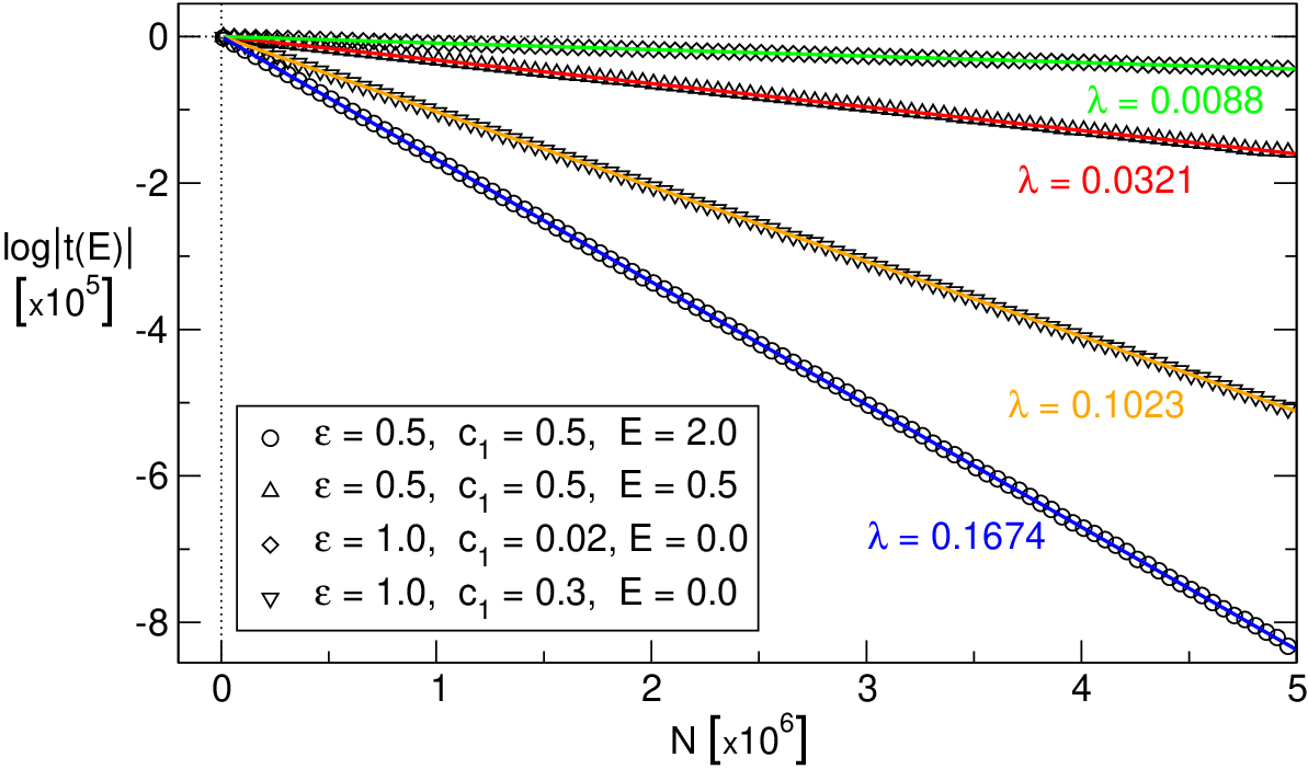


Using the discrete transmission matrix formalism, the scattering amplitudes of a finite chain can be obtained. In figure 4 the logarithm of the modulus of the transmission amplitude is plotted as a function of the length of the system for different binary chains. The exponential decrease of the transmission is clearly observed and the data for finite chains agrees with the value of the Lyapunov exponent obtained from the functional equation in the different cases. In figure 6 the DOS for a finite chain is plotted, showing a fluctuating behaviour around the distribution corresponding to the thermodynamic limit. The evolution of the DOS and the electronic localization length in the thermodynamic limit for a binary chain as a function of the concentrations can be seen in figures 6 and 7. It can be observed how the tools used provide the correct results when the chain is composed of only one species: and inside and outside the allowed energy band respectively and the density of states fits the correct form .
As can be seen in the analysis of the tight-binding Hamiltonian, taking the canonical equation as a starting point a systematic characterization of the electronic properties of the system can be performed, both for finite arrays via the transmission matrix formalism and in the thermodynamic limit with the functional equations.
Aside from the tight-binding model, the functional equation formalism described in this work has been successfully applied by the author and co-workers to other one-dimensional potential models. It has been used to describe the DOS and the localization of the electronic states in the thermodynamic limit of a disordered array of delta potentials [35], as well as to study the significance of binary correlations in the localization and transport properties inside the chain [36][37]. This formalism has revealed itself as a key tool to study other non-trivial 1-D models such as the Pöschl-Teller potential [38][39] which in the disordered configurations exhibits a large amount of exciting properties. We encourage the reader to check the given references since the results there contained are the best proof of the usefulness and power of this methodology.
8 Final discussion
In this work we have compiled and generalized some of the existing methodology to treat disordered quantum wires in one-dimension. The main result of the work is the derivation of a set of universal functional equations that describe analytically the thermodynamic limit of the disordered system independently of the potential model. The equations only depend formally upon the distributions defining the disorder in the system. The derivation of the functional equations has been described in a very detailed way, starting from the transmission matrix of the model and the canonical equation applying to the electronic states in the system. The functional equations can be solved numerically to carry out a systematic and thorough analysis of the electronic properties (DOS, electronic localization, effects of short-range correlations, …) of several models of quantum wires in the thermodynamic limit, as it has already been done by the authors for different one-dimensional potentials [35, 36, 37, 38, 39]. The formalism developed in this work has made it possible to observe several interesting features of the electronic properties of one-dimensional disordered systems such as the fractal nature of the distribution of states in the thermodynamic limit, the appearance of extended states or the drastic change induced by binary short-range correlations in the DOS and the localization of the electrons within the system. The functional equation formalism is not restricted to the framework of the electronic properties of disordered systems, since it can be applied also to other Hamiltonian systems, such as for example one-dimensional spin chains or one-dimensional phonons or excitons, which can be described in terms of a canonical equation of the form (6), where the role of the electronic state is played by a different quantity.
At the present time the theory of disordered systems does not include a unifying mathematical principle comparable to the Bloch theorem for the case of periodic structures. We would like to believe that the derivation of the universal functional equations for disordered systems in one dimension may mean a little advance in this direction. The fact that independently of the potential model it is possible to write a general set of functional equations which only depend on the distributions defining the disorder and that characterize the thermodynamic limit of the systems, is to our minds a result that must be taken into account. And physical relevant quantities such as the DOS or the localization length can be directly calculated in the thermodynamic limit from the functional equations. In spite of their formidable aspect the equations may have analytical solutions in certain cases or they may be useful to extract analytically information of the systems in the thermodynamic limit. Work along this line will probably require the use of a tough mathematical formalism but it could also be very fruitful.
Acknowledgments
I would like to thank my advisor J. M. Cerveró for several illuminating discussions. This research has been partially supported by DGICYT under contracts BFM2002-02609 and FIS2005-01375 and JCyL under contract SA007B05.
Appendix A The transmission matrix
A.1 Properties and symmetries of the transmission matrix
Let be a finite range potential appreciable only inside the region , so that the wave function can be written as
| (67) |
being the linearly independent elementary solutions for each of the continuum spectrum of the potential. By applying the continuity conditions of the state and its derivative at , it is possible to reach an expression of the form
| (68) |
relating the amplitudes of the free particle states on the right and left sides of the potential. is the continuous transmission matrix of the potential and its elements read in a general form:
| (69a) | ||||
| (69b) | ||||
| (69c) | ||||
| (69d) | ||||
where is the Wronskian of the solutions and it must be independent of . A straightforward calculation of the determinant of the transmission matrix leads to
| (70) |
Therefore for all kind of potentials, since no specific assumptions have been made regarding . Let us remark that this property is not a consequence of the time reversal symmetry of the Hamiltonian as it is usually stated. Let us study now the symmetries of the elements of the matrix in different special cases.
A.1.1 Real potential ()
If the potential is real it is always possible to find real linearly independent solutions for each value of the energy . And from equations (69) the following relations hold,
| (71) |
Therefore in the case of a real potential the transmission matrix can be written as
| (72) |
It is easy to check that these matrices satisfy
| (73) |
The latter equation together with define the group .
A.1.2 Complex potential ()
If the potential is complex, it is not possible generally to build functions being real, therefore the conjugation relations (71) are not satisfied. There are no special symmetries among the matrix elements.
| (78) |
with parity symmetry: In the case of a complex potential with parity symmetry, the same analysis as for a real potential can be applied, and equation (76) is obtained, since it does not depend on the elementary solutions being real or complex but only on their symmetries.
| (79) |
with -symmetry: Let us consider a complex local potential invariant under the joint action of parity and time-reversal operations [40]. Then it is possible to find satisfying
| (80) | ||||||
| (81) |
Using the above symmetries in (69) one is led to
| (82) |
Thus the matrix can be written as
| (83) |
A.2 Scattering amplitudes
The scattering amplitudes are directly calculated from the transmission matrix. Figure 8 is a pictorial representation of equation (68).

Considering left incidence then , , , . And it follows
| (84) |
In the case of right incidence , , , . And the equations yield
| (85) |
The insensitivity of the complex transmission amplitude to the incidence direction is trivially proved. Using the properties of the transmission matrix for particular cases of the potential is easy to see that for parity invariant potentials (real or complex) , for generic real potentials and for generic complex ones both amplitudes differ.
In table 1 a summary of the symmetries of the transmission matrices and scattering amplitudes is given for the different type of potentials described.
| Transmission Matrix | Scattering Amplitudes | |
|---|---|---|
| All | ||
| Real | ||
| Real, | ||
| Complex | ||
| Complex, | ||
| Complex, |
A.3 Transmission matrix for a continuous potential
For the most general continuous potential, equation (68) is only satisfied asymptotically, that is the amplitudes of the asymptotic states
| (86a) | ||||
| (86b) | ||||
can be related via the asymptotic transmission matrix ,
| (87) |
The procedure to obtain this asymptotic matrix is the following. First is solving the Schrödinger equation for positive energies so that the more general state reads
| (88) |
in terms of the elementary solutions , . Now one needs to build the asymptotic form of the elementary solutions,
| (89a) | ||||
| (89b) | ||||
Therefore the more general asymptotic state becomes
| (90) |
Equating the coefficients with those corresponding to the asymptotic forms (86) yields
| (91) | ||||||
| (92) |
Solving in terms of one obtains for the elements of the asymptotic matrix
| (93) |
where is the Wronskian of the solutions.
A.3.1 Including a cut-off in the potential
Let us suppose that due to the nature of the potential, it is only appreciable inside the region (figure 1). Then the transfer matrix for the potential with the cut-off relates the amplitudes of the plane waves at and , which can be written from the asymptotic forms (86), yielding the relation
| (94) |
which implies
| (95) |
leading to
| (96) |
Once the asymptotic transmission matrix is known, the cut-off matrix is straightforwardly built. And for a given potential it is usually easier to calculate the asymptotic matrix than to construct directly the cut-off version using the continuity conditions at the cut-off points.
Appendix B The Lyapunov exponents
Let us prove that for a one-dimensional Hamiltonian system, suitable to be described in terms of products of random matrices, the two Lyapunov characteristic exponents (LCE) come in a pair of the form .
Let us consider our system within the discrete transmission matrix formalism. If the Hamiltonian of the system can be written in terms of a potential then it can be shown that the canonical equation takes always the form
| (97) |
where denotes the parameters of the potential at the th site of the system and , are functions depending on these parameters and the energy. Hence the discrete transmission matrix reads
| (98) |
The above matrix becomes a symplectic transformation if but in general . The necessary and sufficient condition to ensure that the LCE of the asymptotic product () are is that the determinant of Oseledet’s matrix equals . Let us remember that . Thus we only need to prove that which is trivial if the individual transfer matrices are symplectic, like for example in the tight-binding model with constant transfer integrals or for the delta potential model, but it may not be so obvious in the most general case. For the proof let us suppose that our system is composed of two different kind of potentials , , in a random sequence. Then the product matrix will contain four different types of matrices, namely , , , according to the different pairs of potentials occurring in the sequence and participating in the canonical equation. Then,
| (99) |
being the number of times that appears, and the frequencies of appearance of the pairs in the thermodynamic limit. From (98) it readily follows
| (100) |
A simple reflection symmetry argument requires that so the above expression equals . And finally the eigenvalues of must be of the form .
This proof can be straightforwardly extended for a case considering different potentials or for a continuous model with parameters inside a certain range with a given probability distribution.
This result about the Lyapunov exponent for a one-dimensional system must be naturally expected, by the fact that the same physical problem can be treated through the continuous transmission matrix formalism and it must lead to the same results. Therefore considering the latter matrices which have always determinant unity, it is obvious that .
Appendix C DOS from node counting
James and Ginzbarg obtained the expression of the integrated density of states (IDOS) of a linear chain of potentials in terms of the changes of sign of the wave function inside the different sectors of the system [41]. Their reasoning is the following. Let us consider a binary wire composed of two types of potentials and . And let be the th sector of the chain including a potential. Then the elementary solutions for positive energy in this cell , , can be chosen to satisfy
| (101a) | ||||||
| (101b) | ||||||
Now let us consider a certain energy for which has nodes inside the given sector (the first one at ). Then for this energy, possible states include with zeros and with zeros in the cell (for sufficiently small ). For low , and as the energy grows the index increases by one whenever . Thus the energy spectrum can be divided in intervals according to the value of the index , so that if lies in the interval labelled with then the solution will have or nodes in every sector of type . To determine whether the number of zeros is or , one has to check if and have the same signs (even number of nodes) or opposite signs (odd number of nodes). Thus for that energy the number of nodes in a sector can be written as
| (102) |
where if and have the same signs and otherwise. The same reasoning can be used for the species . And for an energy with the labels for the species and for , the total number of nodes inside the mixed system and therefore the IDOS per atom reads
| (103) |
where , , are the concentrations of the species and , , are the concentrations of changes of sign for each species, that is the number of cells containing a certain species in which the state changes sign (i.e. has opposite signs at the beginning and at the end of the sector) divided by the total number of potentials of the system. To obtain the density of states one needs to evaluate in the interval ) in which the indices , , can be considered to remain fixed. Therefore the only quantities that can vary in the differential interval are the concentrations of changes of sign. Hence,
| (104) |
And this expression is straightforwardly generalized for an arbitrary number of species. The main result is that to determine the DOS correctly, depending on the energy range one has to sum or subtract the changes of sign of the wave function at sectors corresponding to different species.
Now let us see how one can know the indices , , in a practical way. The system is completely determined by the canonical equation
| (105) |
The functions , , can be obtained in terms of the elementary solutions of the Schrödinger equation in each sector of the chain. Making use of equations (69) and (9) the function can be defined as
| (106) |
where are the elementary solutions in the th sector with a potential of type . Imposing the additional conditions (101) it follows for the case that . That is, the function takes the same values that the elementary solution , verifying equations (101), would reach at the end of every sector. Thus, whenever as a function of the energy changes its sign, and therefore the index increases by , also registers a change of sign. What is more, it is not hard to see that in equation (104) the terms , , can be directly identified with the signs of . And finally, one can write
| (107) |
From a numerical viewpoint one must do the transmission of the state through the system using the functional equation and count the number of changes of sign from site to site for the different atomic species, to perform finally a numerical differentiation with respect to the energy and sum or subtract the different contributions of the species according to the sign of the function for the energy considered.
References
- [1] Anderson, P.W.: Absence of difussion in certain random lattices. Phys. Rev. 109, 1492-1505 (1958)
- [2] Flores, J.C.: Transport in models with correlated diagonal and off-diagonal disorder. J. Phys.: Condens. Matter 1, 8471-8479 (1989)
- [3] Dunlap, D.H., Wu, H.-L. and Phillips, P.W.: Absence of localization in a Random-Dimer model. Phys. Rev. Lett. 65, 88-91 (1990)
- [4] Sánchez, A., Maciá, E. and Domínguez-Adame, F.:Suppression of localization in Kronig-Penney models with correlated disorder. Phys. Rev. B 49, 147-157 (1994)
- [5] Hilke, M.: Localization properties of the periodic random Anderson model. J. Phys. A: Math. Gen. 30, L367-L371 (1997)
- [6] Izrailev, F.M. and Krokhin, A.A.: Localization and the mobility edge in one-dimensional potentials with correlated disorder. Phys. Rev. Lett. 82, 4062-4065 (1999)
- [7] de Moura, F.A.B.F. and Lyra, M.L.: Delocalization in the 1D Anderson model with long-range correlated disorder Phys. Rev. Lett. 81, 3735-3738 (1998)
- [8] Bellani,V., Diez, E., Hey, R., Tony, L., Tarricone, L., Parravicini, G.B., Domínguez-Adame, F. and Gómez-Alcalá, R.: Experimental Evidence of delocalized states in random dimer superlattices. Phys. Rev. Lett. 82, 2159-2162 (1999)
- [9] Krokhin, A., Izrailev, F., Kuhl, U., Stöckmann, H.J. and Ulloa, S.E.: Random 1D structures as filters for electrical and optical signals. Physica E 13, 695-698 (2002)
- [10] Kuhl, U., Izrailev, F.M., Krokhin, A.A. and Stöckmann, H.J.: Experimental observation of the mobility edge in a waveguide with correlated disorder. Appl. Phys. Lett. 77, 633-635 (2000)
- [11] Deych, L.I., Erementchouk, M.V. and Lisyansky, A.A.: Scaling in one-dimensional Anderson localization problem in the region of fluctuation states. Phys. Rev. Lett. 90, 126601 (2003)
- [12] Deych, L.I., Lisyansky, A.A. and Altshuler, B.L.: Single parameter scaling in one-dimensional localization revisited. Phys. Rev. Lett. 84, 2678-2681 (2000)
- [13] Deych, L.I., Erementchouk, M.V. and Lisyansky, A.A.: Scaling properties of the one-dimensional Anderson model with correlated diagonal disorder. Phys. Rev. B 67, 024205 (2003)
- [14] Ahmed, Z.: Schrödinger transmission through one-dimensional complex potentials. Phys. Rev. A 64, 042716 (2001)
- [15] Beam, J.E.: Multiple reflection in potential-barrier scattering. Am. J. Phys. 38, 1395-1401 (1970)
- [16] Maciá, E. and Domínguez-Adame, F.: Electrons, phonons and excitons in low dimensional aperiodic systems. Editorial Complutense, 2000
- [17] Izrailev, F.M., Kottos, T. and Tsironis, G.P.: Hamiltonian map approach to resonant states in paired correlated binary alloys. Phys. Rev. B 52, 3274-3279 (1995)
- [18] Izrailev, F.M., Ruffo, S. and Tessieri, L.: Classical representation of the one-dimensional Anderson model. J. Phys. A: Math. Gen. 31, 5263-5270 (1998)
- [19] Tabor, M.: Chaos and integrability in nonlinear dynamics: an introduction. John Wiley & Sons, 1989
- [20] Kramer, B. and MacKinnon, A.: Localization: theory and experiment. Rep. Prog. Phys. 56, 1469-1564 (1993)
- [21] Crisanti, A., Paladin, G. and Vulpiani, A.: Products of Random Matrices in Statistical Physics. Springer-Verlag, 1993
- [22] Arnold, L.: Random Dynamical Systems. Springer-Verlag, 1998
- [23] Kirkman, P.D. and Pendry, J.B.: The statistics of one-dimensional resistances. J. Phys. C 17, 4327-4344 (1984)
- [24] Johnson, R. and Kunz, H.: The conductance of a disordered wire. J. Phys. C 16, 3895-3912 (1983)
- [25] Canisius, J. and van Hemmen, J.L.: Localisation of phonons. J. Phys. C 18, 4873-4884 (1985)
- [26] Dean, P.: The vibrational properties of disordered systems: numerical studies. Rev. Mod. Phys. 44, 127-168 (1972)
- [27] Lee, P.A. and Ramakrishnan, T.V.: Disordered electronic systems. Rev. Mod. Phys. 57, 287-337 (1985)
- [28] Dyson, F.J.: The dynamics of a disordered linear chain. Phys. Rev. 92, 1331-1338 (1953)
- [29] Schmidt, H.: Disordered one dimensional crystals. Phys. Rev. 105, 425-441 (1957)
- [30] Agacy, R.L.: The vibrational spectrum of a disordered linear system. Proc. Phys. Soc. 83, 591-596 (1964)
- [31] Borland, R.E. and Bird, N.F.: A calculation of the density of electron states and degree of localization in a one-dimensional liquid model. Proc. Phys. Soc. 83, 23-29 (1964)
- [32] Dean, P.: Vibrations of glass-like disordered chains. Proc. Phys. Soc. 84, 727-744 (1964)
- [33] Agacy, R.L. and Borland, R.E.: The electronic structure of a one dimensional random alloy. Proc. Phys. Soc. 84, 1017-1026 (1964)
- [34] Gubernatis, J.E. and Taylor, P.L.: Special aspects of the electronic structure of a onedimensional random alloy. J. Phys. C 4, L94-L96 (1971)
- [35] Cerveró, J.M. and Rodríguez, A.: Infinite chain of N different deltas: a simple model for a quantum wire. Eur. Phys. J. B 30, 239-251 (2002)
- [36] Cerveró, J.M. and Rodríguez, A.: Simple model for a quantum wire II. Statistically correlated disorder. Eur. Phys. J. B 32, 537-543 (2003)
- [37] Cerveró, J.M. and Rodríguez, A.: Simple model for a quantum wire III. Transmission in finite samples with correlated disorder. Eur. Phys. J. B 43, 543-548 (2005)
- [38] Cerveró, J.M. and Rodríguez, A.: Absorption in atomic wires. Phys. Rev. A 70, 052705 (2004)
- [39] Rodríguez, A. and Cerveró, J.M.: Continuum of extended states in the spectrum of a one-dimensional random potential. Phys. Rev. B 72, 193312 (2005)
- [40] Muga, J.G., Palao, J.P., Navarrro, B. and Egusquiza, I.L.: Complex absorbing potentials. Phys. Rep. 395, 357-426 (2004)
- [41] James, H. and Ginzbarg, A.: Band structure in disordered alloys and impurity semiconductors. J. Phys. Chem. 57, 840-848 (1953)