Entanglement in Graph States and its Applications

Marc Hein Affiliation: Institut für Theoretische Physik, Universität Innsbruck, Technikerstraße 25, A-6020 Innsbruck, Austria
Institut für Quantenoptik und Quanteninformation der Österreichischen Akademie der Wissenschaften, Technikerstraße 21a, A-6020 Innsbruck, Austria Wolfgang Dür Jens Eisert Robert Raussendorf Maarten Van den Nest Hans Jürgen Briegel

1 Introduction

The recognition of the key role entanglement plays in the understanding of the radical departure of quantum from classical physics came historically remarkably late. In the early years of quantum mechanics starting from the mid twenties of the last century, often referred to as the ‘golden years’, this aspect was not quite in the center of activities: Researchers were occupied with successfully applying the new theory to a wide range of physical phenomena, continuously adding to the impressive list of theoretical studies matching experimental findings. It was not until the year 1935, when Einstein, Podolsky and Rosen expressed their dissatisfaction with the state of the theory, constructing a Gedanken experiment involving a measurement setup in a ‘separated laboratories paradigm’ that should identify the description provided by quantum mechanics as incomplete EPR35. This Gedanken experiment involved local measurements on constituents of a composite quantum system prepared in an entangled state in a distributed setup. In the same year, Schrödinger, also one of the major contributors to the theory, formulated some of the mathematical implications of entanglement on the statistics of measurement outcomes; and actually coined the term ‘entanglement’ both German and in English schroedinger35. The program envisioned by Einstein and colleagues – to demonstrate the incompleteness of a quantum mechanical description – may be fairly said to have essentially failed. They nevertheless could pinpoint the aspect of quantum theory in which it would crucially depart from a local classical statistical theory.

This was fully realized in the 1960ies, when Bell reconsidered the situation discussed by Einstein, Podolsky and Rosen, restated in a setting involving spin- $1/2$ degrees of freedom due to Bohm Bohm51. He demonstrated the validity of bounds to correlation functions of measurement outcomes of dichotomic measurements, provided that they would be resulting from a ‘local realistic model’, meaning from a local classical statistical theory Bell64. These bounds are indeed violated by the predictions of quantum mechanics. After the advent of reliable sources of entangled states, many experiments were performed, all consistent with the predictions of quantum theory, and none with the bounds put forth in form of Bell’s inequalities (see, e.g., ref. As81, Zei99). It can be said that it is in the role of entanglement where the departure of quantum from classical physics is most manifest, indicating that the intrinsic randomness in quantum theory can not be thought of as resulting from mere classical ignorance in an underlying classical statistical theory.

In the meantime, it has become clear that entanglement plays a central role also from a different perspective: it can serve as an essential ingredient in applications of quantum information processing NielsenBook. For example, entanglement is required for an established key to be unconditionally secure in quantum key distribution BB84, Ekert91, Shor00, Curty04. Entanglement is also believed to be responsible for the remarkable speedup of a quantum computer compared to classical computers Braunstein99, Lloyd00, JL02, Miy01, Vidal03, the underlying logic of which being based on the laws of classical physics Feynman, Deutsch, Shor97, Grover.

Formally, entanglement is defined by what it is not: a quantum state is called entangled, if it is not classically correlated. Such a classically correlated state is one that – in the distant laboratories paradigm – can be prepared using physical devices locally, where all correlations are merely due to shared classical randomness. The kind of correlations in such preparations are hence of the same origin as ones that one can realize in classical systems by means of communicating over telephone lines. This is in sharp contrast to the situation in entangled states, which cannot be produced using local physical apparata alone. This facet of entanglement hence concentrates on the preparation procedure. The concept of distillable entanglement IBMPure in turn grasps directly entanglement as a resource, and asks whether maximally entangled states can be extracted, distilled, within a distant laboratories paradigm.

Part of the theoretical challenge of understanding entanglement lies in the fact that is also (at least partly) responsible for the quantum computational speedup: state space is big. The dimension of state space, the set of all quantum states corresponding to legitimate preparation procedures, grows very rapidly with the number of constituents in a composite quantum system. In fact, it grows exponentially. Consequently, in the whole development of quantum information theory, it has been a very useful line of thought to investigate situations where the involved quantum states could be described with a smaller number of parameters, while still retaining the essential features of the problem at hand. So certain ‘theoretical laboratories’ facilitated the detailed investigation of phenomena, properties, and protocols that arise in quantum information theory, while keeping track of a set of states that is at most polynomially growing in dimension. So-called stabilizer states Gottesman, NielsenBook, Werner states We89, matrix-product states MPS, or quasi-free states Gaussian are instances of such ‘laboratories’. In the center of this review article are the graph states, the structure of which can be described in a concise and fruitful way by mathematical graphs. They have been key instrumental tools in the development of models for quantum computing, of quantum error correction, and of grasping the structure of bi- and multi-partite entanglement.

Graph states are quantum states of a system embodying several constituents, associated with a graph¹¹ 1 Note that in the literature one finds several inequivalent concepts of quantum states that are in one way or another associated with graphs Graph, Graph2. For example, entanglement sharing questions have been considered in a multi-partite quantum system based on quantum states defined through mathematical graphs, see refs. Rings, Buzek, Zanardi, Parker.. This graph may be conceived as an interaction pattern: whenever two particles, originally spin- $1/2$ systems, have interacted via a certain (Ising) interaction, the graph connecting the two associated vertices has an edge. Hence, the adjacency matrix of a simple graph, a symmetric $N\times N$ matrix for a system consisting of $N$ qubits with entries taken from $\{0,1\}$ , fully characterizes any graph state at hand Briegel01, OneWay3, He04, Du03a, Nest04a. In this sense the graph can be understood as a summary of the interaction history of the particles. At the same time, the adjacency matrix encodes the stabilizer of the states, that is, a complete set of eigenvalue equations that are satisfied by the states ²² 2 In some sense, this graphical representation plays a similar pedagogical role as Feynman diagrams in quantum electrodynamics: The latter provide an intuitive description of interaction processes in spacetime, but, at the same time, they have a concise mathematical meaning in terms of the corresponding propagator in an expansion of the scattering operator.. Thus graph states are actually stabilizer states Gottesman. This class of graph states play a central role in quantum information theory indeed.

To start with, graph states form a universal resource for quantum computing based on measurements OneWay1, OneWay2, OneWay3, OneWay5. In such one-way computing, one starts off with a cluster state, which is a specific instance of a graph state, and performs von-Neumann measurements at single sites associated with vertices. In fact, it was in the form of such cluster states Briegel01, when graph states have first been considered, in a narrower sense, with respect to a graph reflecting a cubic lattice. On the subspace that is retained any unitary can be implemented, thereby realizing universal computation without the need of making use of any controlled two-system quantum gates. The cluster state hence forms a universal resource for quantum computation. The performed measurements introduce a probabilistic aspect to the scheme; yet, the overall set-up of the one-way computer is deterministic, as the process can be de-randomized by means of appropriate local unitaries taken from the Pauli group applied before the readout step OneWay1, OneWay3.

Such one-way computing is interesting at least from two perspectives: on the one hand, it provides a computational model OneWay2 different from the original gate-based model, which resembles more closely the gate model of classical computation. In fact, questions of complexity and simulatability often become more transparent in the picture of the one-way computer than in the gate model. For instance, operations from a certain set of operations, the so-called Clifford operations NielsenBook, can be kept track of classically in an efficient manner. When measuring Pauli operators in the course of the computation, the states of the whole system will be a sequence of graph states that can be described by a sequence of adjacency matrices OneWay3. However, if in the first step of the gate-based model, a non-Clifford operation is applied, unlike in the picture of the one-way computer, it is no longer obvious in the gate-model that the dynamics of the rest of the network can be described efficiently.

On the other hand, there are good reasons to believe that the undoubtedly tremendous challenges associated with actually realizing a quantum computer can be lessened when relying on an architecture based on graph states. In many quantum systems in a lattice, nearest-neighbor interactions are natural, rendering the preparation of cluster states through one dynamical process a relatively feasible step. Furthermore, and maybe more importantly, one realizes a certain distinction between the process of creating entanglement and the process of consuming it. Hence, even if one exploits a lossy or even probabilistic process in order to prepare the graph states, in many set-ups one can, in principle, end-up with graph states free of errors, then to be used as a resource of the actual computation. Even if the entangling operations are themselves faulty, e.g. subject to photon loss in a linear optical implementation, fault tolerant schemes can be devised, in principle up to a loss rate of several tens of percents.

In quantum-gate-based quantum computation, graph states also play a prominent role as codewords in quantum error correction, allowing for reliable storage and processing of quantum information in the presence of errors. This is done by appropriately encoding quantum information in quantum states of a larger number of quantum systems. This is the second branch how the concept of graph states originally came into play, namely in form of graph codes Schlinge02a, SchlingeHabilschrift. These instances of quantum codes are determined by the underlying graph.

Finally, the idea of the ‘theoretical laboratory’ itself allows for a wide range of applications. Aspects of bi-partite and, in particular, multi-partite entanglement are typically extraordinarily hard to grasp Du99. This is again partially due to the fact that state space is so rapidly increasing in dimension with a larger number of constituents. The decision problem whether a mixed state is entangled or classically correlated is already provably a computationally hard problem in the dimension of the constituents. Apart from the classification of multi-particle entanglement, even for pure states, a complete meaningful quantification of multi-particle entanglement is yet to be discovered LiPo98. Already at the origin is the question in what units to phrase any result on quantification matters: there is no multi-particle analog of the maximally entangled pair of spin- $1/2$ -particles, to which any pure bi-partite entanglement is equivalent: any pure state can be transformed into such maximally entangled pairs in an asymptotically lossless manner, one of the key results of entanglement theory pureState, Th02. This means that the achievable rate of distillation and formation is the same. The multi-partite analogue of such a reversible entanglement generating set (as it is formed by the maximally entangled qubit pair in the bi-partite setting) has not yet been identified, at least none that has a finite cardinality³³ 3 For a brief review on multi-particle entanglement, see, e.g., ref. Eisert05..

Within the setting of graph states, some of the intriguing questions related to aspects of multi-particle entanglement can be addressed, expressing properties of entanglement in terms of the adjacency matrix. Central tasks of interconverting different forms of multi-particle entanglement, in particular of ‘purifying’ it, can and have been studied: here, the aim is to extract pure graph states from a supply of noisy ones, having become mixed through a decoherence process Du03a. Based on such purification protocols, even protocols in quantum cryptography have been devised, making use of the specific structure of this class of quantum states Lo04, Du05c. In turn, graph states form an ideal platform to study the robustness of multi-particle entangled states under such in realistic settings anyway unavoidable decoherence processes. In a nutshell, multi-particle entangled states may exhibit a surprising robustness with respect to decoherence processes, independent from the system size Du04b. Finally, questions of inconsistency of quantum mechanics with local classical statistical theories become very transparent for graph states Gue04. In all of the above considerations, the class of graph states is sufficiently restricted to render a theoretical analysis feasible, yet often complex enough to appropriately grasp central aspects of the phenomenon at hand.

Departing slightly from the original formulation, weighted graph states have been considered CDHB05, where the interaction is no longer a fixed Ising interaction with a constant weight. Such states can be thought of as resulting from a semi-classical Boltzmann gas: classical particles carrying a quantum spin- $1/2$ degree of freedom would in an idealized description give rise to such a graph state through collision of particles. Such weighted graph states find numerous applications in the description of random quantum systems. They can also be taken as a basis set of states to approximate ground states of many-body systems in a variational principle. Owing the structural similarity to the fact that mathematically, discrete and continuous Weyl systems have so much in common, graph states in harmonic infinite-dimensional quantum systems have finally been studied that resemble very much the situation of graph states for finite-dimensional quantum systems HC, Pl04.

This review article aims at providing a self-contained introduction to the theory of graph states in most of these aspects, both conceived as a tool and as a central resource in quantum information theory in their own right. We will introduce the basic notions of graph states, discuss possible descriptions of their entanglement content, their interconversion and purification, and various applications in the context of quantum information science.

1.1 Outline

We start with a detailed introduction of graph states, whose entanglement properties are analyzed in the following chapters. After setting basic notations in sec. 1.2 that are frequently used throughout this article, we give essentially two alternative definitions for graph states in sec. 2, namely, in terms of the underlying interaction pattern and in terms of the stabilizer. We illustrate how elementary properties of a graph state and basic operations, such as (Pauli) measurements, on these states, can be phrased concisely in terms of the underlying graph. It is shown that the action of Clifford operations on graph states (sec. 3) and the reduced states for graph states (sec. 6) can be determined efficiently from the underlying graph. These relations will allow for a classification of graph states in sec. 7 and for an efficient computation of entanglement properties in sec. 8. We discuss some examples and applications to quantum error correction, multi–party quantum communication, and quantum computation in sec. 4. We briefly discuss some generalizations of graph states in the language of discrete Weyl systems in sec. 2. Sec. 5 contains also a short review about possible realizations of graph states in physical systems.

In sec. 7 we will then discuss the classification of graph states in terms of equivalence classes under different types of local operations and provide a complete classification for graph states with up to seven vertices. The results indicate that graph states form a feasible and sufficiently rich class of multi-party entangled states, which can serve as good starting point for studies of multi-party entanglement.

In sec. 8 we discuss various aspects of entanglement in graph states. We briefly review some results about the ‘non-classicality’ of graph states and how their entanglement can be detected with Bell inequalities. The genuine multi-particle entanglement of graph states is characterized and quantified in terms of the Schmidt measure, to which we provide upper and lower bounds in graph theoretical terms.

Finally, we introduce two possible extensions of graph states. On the one hand, in sec. 9 the class of weighted graph states is introduced, which comprises particles that interact for different times and provides an interesting model for the study of the entanglement dynamics in many–particle systems. Here, we consider $N$ initially disentangled spins, embedded in a ring or $d$ -dimensional lattice of arbitrary geometry, which interact via some long–range Ising–type interaction. We investigate relations between entanglement properties of the resulting states and the distance dependence of the interaction in the limit $N\to\infty$ and extend this concept to the case of spin gases.

On the other hand, in sec. 10, graph diagonal states serve as standard forms for mixed states and occur naturally whenever pure graph states are exposed to decoherence. We show that the lifetime of (distillable) entanglement for GHZ-type superposition states decreases with the size of the system, while for a class of other graph states the lifetime is independent of the system size. These results are largely independent of the specific decoherence model. Finally, the concept of entanglement purification is applied to graph states and possible applications to quantum communication are described.

1.2 Notations

Refer to caption — Figure 1: This ring depicts a graph with $7$ vertices

At the basis this review article lies the concept of a graph Graph, Graph2. A graph is a collection of vertices and a description which of the vertices are connected by an edge. Each graph can be represented by a diagram in a plane, where a vertex is represented by a point and the edges by arcs joining two not necessarily distinct vertices. In this pictorial representation many concepts related to graphs can be visualized in a transparent manner. In the context of the present article, vertices play the role of physical systems, whereas edges represent an interaction. Formally, an (undirected, finite) graph is a pair

G=(V,E)

(1)

of a finite set $V=\{1,\ldots,N\}$ and a set $E\subset[V]^{2}$ , the elements of which are subsets of $V$ with two elements each Graph. The elements of $V$ are called vertices, the elements of $E$ edges. In the following, we will mainly consider simple graphs. A simple graph contains neither loops (edges connecting vertices with itself) nor multiple edges. We also regard a generalization of these simple graphs, where each edge $\{a,b\}$ is associated with a weight $\varphi_{ab}$ representing the strength of the respective interaction. Although the concept of a weighted graph is more general than that of a simple graph, we will use the notion of a graph in the more narrow sense of a simple graph, unless we explicitly mention that a certain section is devoted to weighted graphs.

Since there are in general

\tbinom{N}{2}=\tfrac{N(N-1)}{2}

(2)

different possibilities for choosing set of edges $E$ in a graph of $|V|=N$ vertices, the number of distinct graphs is $2^{\tbinom{N}{2}}$ . Graph theory is mostly interested in problems that are invariant under permutations of the vertices, when these permutations respect the neighborhood relation, i.e., map neighbored vertices onto neighbored vertices. Such permutations are called graph isomorphisms. Two graphs $G_{1}=(V_{1},E_{1})$ and $G_{2}=(V_{2},E_{2})$ are called isomorphic if there exists a bijection $f:V_{1}\mapsto V_{2}$ such that

\{a,b\}\in E_{1}\hskip 28.45274pt\Longleftrightarrow\hskip 28.45274pt\{f(a),f(b)\}\in E_{2}\;.

(3)

Note that the number of non-isomorphic graphs still grows exponentially with the number $N$ of vertices Harary73.

Vertices $a,b\in V$ that are the endpoints of an edge are referred to as being adjacent. The adjacency relation gives rise to an adjacency matrix $\mathbf{\Gamma}_{G}=\mathbf{\Gamma}$ associated with a graph. $\mathbf{\Gamma}$ is a symmetric $N\times N$ -matrix, with elements

\mathbf{\Gamma}_{ab}=\left\{\begin{array}[]{ll}1,&\text{ if $\{a,b\}\in E$,}\\ 0&\text{otherwise}.\end{array}\right.

(4)

In the case of weighted graphs, the adjacency matrix also specifies the weights of the edges, i.e., $\mathbf{\Gamma}_{ab}=\varphi_{ab}$ . We will make repeated use of the neighborhood

N_{a}:=\left\{b\in V\,|\,\{a,b\}\in E\right\}

(5)

of a given vertex $a\in V$ . The neighborhood is the set of vertices adjacent to a given vertex. The number $|N_{a}|$ of neighbors is called the degree of the vertex $a$ . A vertex $a\in V$ of degree $|N_{a}|=0$ will be called an isolated vertex. An $\{a,b\}$ -path is an ordered list of vertices $a=a_{1},a_{2},\ldots,a_{n-1},a_{n}=b$ , such that $a_{i}$ and $a_{i+1}$ are adjacent for all $i$ . A connected graph is a graph that has an $\{a,b\}$ -path for any two $a,b\in V$ . Otherwise it is referred to as disconnected .

When a vertex $a$ is deleted in a graph $G$ , together with all edges incident with $a$ , one obtains a new graph, denoted by $G\setminus a$ . For a subset of vertices $U\subset V$ of a graph $G=(V,E)$ let us denote with $G\setminus U$ the graph that is obtained from $G$ by deleting the set $U$ of vertices and all edges which are incident with an element of $U$ . In a mild abuse of notation, we will also write $G\setminus F$ for the graph that results from a deletion of all edges $e\in F$ , where $F\subset E\subset[V]^{2}$ is a set of edges. For a set of edges $F\subset[V]^{2}$ we will write $G\cup F:=(V,E\cup F)$ and $G+F:=(V,E+F)$ , where

E+F=(E\cup F)\setminus(E\cap F)

(6)

is the symmetric difference of $E$ and $F$ . Note that the symmetric difference corresponds to the addition modulo $2$ or the component-wise XOR if the sets are considered as binary vectors over the integer field $\mathbb{F}_{2}$ modulo two . Similarly, an induced subgraph $G[A]$ of a graph $G=(V,E)$ , where $A\subset V$ , is obtained by deleting all vertices (and the incident edges) that are not contained in $A$ .

Graphs may be colorable. A proper two-coloring of a graph is a labeling $V\longrightarrow\{1,2\}$ , such that all adjacent vertices are associated with a different element from $\{1,2\}$ , which can be identified with two colors. In graph theory these graphs are also called ‘bi-partite graphs’, since the set of vertices can be partitioned into two disjoint sets, often called sinks or sources, such that no two vertices within the same set are adjacent. It is a well known fact in graph theory that a graph is two-colorable if and only if (iff) it does not contain any cycles of odd length.

In the remainder of this article each vertex stands for a two–level quantum system $\mathbf{H}^{a}\simeq\mathbb{C}^{2}$ or qubit. The state vector of the single–qubit system $\mathbf{H}^{a}$ can be written as $|\psi\rangle^{a}=\alpha|0\rangle^{a}+\beta|1\rangle^{a}$ with $|\alpha|^{2}+|\beta|^{2}=1$ . The vectors $|0\rangle$ and $|1\rangle$ are the eigenvectors of the Pauli matrix $\sigma_{z}$ with eigenvalue $+1$ and $-1$ . The matrices $\sigma^{a}_{0}=\mathbf{1}_{a}$ , $\sigma^{a}_{1}=\sigma_{x}^{a}$ , $\sigma^{a}_{2}=\sigma_{y}^{a}$ and $\sigma^{a}_{3}=\sigma_{z}^{a}$ are the Pauli matrices of this two–level system, where the upper index specifies the Hilbert space on which the operator acts. Note that these operators form an orthogonal basis of Hermitian operators with respect to the scalar product $\langle A,B\rangle:=\text{tr}(A^{\dagger}B)$ . Up to the phase factors $\pm 1$ and $\pm i$ they also generate the Pauli group $\mathcal{P}:=\langle\{\pm 1,\pm i\}\times\{\sigma_{0},\sigma_{x},\sigma_{y},\sigma_{z}\}\rangle$ . We will frequently use the projectors onto the eigenvectors of the Pauli operators. For example,

P^{a}_{z,\pm}=\frac{1\pm\sigma_{z}^{a}}{2}

(7)

denotes the projector onto the eigenvector $|z,\pm\rangle$ of $\sigma_{z}^{a}$ with eigenvalue $\pm 1$ (similarly for $\sigma_{x}^{a}$ and $\sigma_{y}^{a}$ ).

To simplify notations, we use subsets $U\subseteq V$ as an upper index for states, operators and sets. They denote the respective tensor product of a given state or sets, e.g.

|+\rangle^{V}=\bigotimes_{a\in V}|+\rangle^{a}\hskip 19.91684pt\text{or}\hskip 19.91684pt\mathcal{P}^{V}=\bigotimes_{a\in V}\mathcal{P}^{a}\;,

(8)

where $|+\rangle=\frac{1}{\sqrt{2}}\left(|0\rangle+|1\rangle\right)$ . The subsets are also used to label those vertices where the operator acts non-trivially, for example

\sigma_{z}^{U}=\bigotimes_{b\in U}\sigma_{z}^{b}\;.

(9)

Moreover, we identify sets $U$ and their corresponding binary vectors $U=(U_{b})_{b\in V}\simeq(U_{1},\ldots,U_{N})$ over the binary field $\mathbb{F}_{2}^{V}$ with the same symbol. Finally, $a$ refers to both the vertex and the corresponding one-element set $\{a\}$ ensuring that $\sigma_{x}^{a}\equiv\sigma_{x}^{\{a\}}$ . These notations allow us to use set and binary operations in the same formula. For example, for $A,B\in\mathcal{P}(V)\cong\mathcal{F}_{2}^{V}$ we will write $A\cup B$ , $A\cap B$ and $A\setminus B$ ( $\bar{A}:=V\setminus A$ ) for the union, intersection and difference (complement) as well as $A+B$ and $\langle A,B\rangle$ for the addition and the scalar product modulo $2$ .

In the multi-partite case one can group the vertices into different partitions and, for example, study the entanglement with respect to these partitions. Here, any tuple $(A_{1},...,A_{M})$ of disjoint subsets $A_{i}\subset V$ with $\bigcup^{M}_{i=1}A_{i}=V$ will be called a partition of $V$ . We will write

(A_{1},...A_{M})\leq(B_{1},...,B_{M^{\prime}}),

(10)

if $(A_{1},...A_{M})$ is a finer partition than $(B_{1},...,B_{M^{\prime}})$ . which means that every $A_{i}$ is contained in some $B_{j}$ . The latter is then a coarser partition.

2 Definitions for graph states

With the notations introduced in the previous section we can provide some definitions for graph states. Throughout this article, we mainly consider two alternative descriptions. Most naturally, graph states can be regarded as the result of an interaction of particles initially prepared in some product state. Certainly not all imaginable interaction patterns can be represented reasonably by a simple graph. In sec. 2.1 we introduce the description of graph states in terms of the interaction pattern and show that such a definition is also meaningful if all particles interact with the same Ising-type interaction but possibly for different interaction times. This description generalizes to so called weighted graph states, which are introduced in sec. 9. The alternative definition proposed in sec. 2.2, on the other hand, is restricted to the class of states that correspond to a simple graph. Such states can be described efficiently in terms of their stabilizer, which is a subgroup of the Pauli group. We briefly address the question of local unitary equivalence, discuss the relation to stabilizer states and illustrate an alternative representation of the stabilizer formalism in terms of its binary representation⁴⁴ 4 Although the remainder of the article will not be based on the binary representation.. We sketch a possible extension of the stabilizer formalism to $d$ -level systems and finally summarize further alternative approaches to graph states in sec. 2.3.

2.1 Interaction pattern

In this subsection we give a careful motivation for the concept of graph states in terms of interaction patterns, concluding with a precise definition given at the end of this subsection. Let us consider a set of $2$ -level systems (qubits) that are labeled by the vertices $V$ of a graph $G=(V,E)$ . The qubits are prepared in some initial state vector $|\Psi\rangle$ and then are coupled according to some interaction pattern represented by the graph $G$ . For each edge $\{a,b\}\in E$ the qubits of the two adjacent vertices $a$ and $b$ interact according to some (non-local) unitary $U_{ab}=e^{-i\varphi_{ab}H_{ab}}$ . Here, $H_{ab}$ denotes the interaction Hamiltonian and $\varphi_{ab}$ represents the coupling strength or (with appropriate physical units) the interaction time. The most general of such setups, in which the qubits can interact according to different $2$ -body interactions $H_{ab}$ , has to be described by graphs, whose edges carry a labeling that specifies both the different unitaries $U_{ab}$ as well as the ordering in which interactions occur.

Under which conditions can the outcome of this interaction pattern be completely specified by a simple graph $G$ ? If the graphs shall give a sufficient characterization for a large class of interaction patterns, we can pose the following constraints:

(1)

Since the graph $G$ does not provide any ordering of the edges, all two–particle unitaries $U_{ab}$ involved must commute:

$[U_{ab},U_{bc}]=0\hskip 28.45274pt\forall a,b,c\in V\;.$ (11)
(2)

Because we deal with undirected graphs⁵⁵ 5 In a directed graph the set of edges $E$ is given by ordered pairs $(a,b)$ . The order implies that vertices $a$ and $b$ are connected by a directed edge from $a$ to $b$ ., the unitaries must be symmetric:

$U_{ab}=U_{ba}\hskip 28.45274pt\forall a,b\in V\;.$ (12)
(3)

If the edges are not further specified by weights, all qubits should interact through the same two–particle unitary $\mathbf{U}$ :

$U_{ab}=\mathbf{U}^{\{a,b\}}\hskip 28.45274pt\forall a,b\in V\;.$ (13)

In the case of qubits condition (1) is already sufficient to restrict the analysis of particles to the case where the qubits interact according to the same Ising interaction, e.g. $H^{I}_{ab}=\sigma_{z}^{a}\sigma_{z}^{b}$ . This statement is reflected in the following proposition.

Proposition 1 (Standard form for commuting interactions)

With an appropriate choice of the local basis in each individual qubit system, any set of commuting two–particle unitaries, i.e., the unitaries fulfill (1), does only contain interactions of the form

\varphi_{ab}\,H_{ab}=\varphi_{ab}\,\sigma_{z}^{a}\sigma_{z}^{b}+\alpha_{a}\,\sigma_{z}^{a}+\alpha_{b}\,\sigma_{z}^{b}\;.

(14)

In other words, any interaction pattern in which the qubits interact according to some two–particle unitaries chosen from a set of commuting interactions, is up to local $z$ -rotations⁶⁶ 6 I.e., $V^{a}=e^{i\beta_{a}\sigma_{z}^{a}}$ to be performed before or after the interaction pattern. an Ising interaction pattern

U^{I}_{ab}(\varphi_{ab}):=e^{-i\,\varphi_{ab}\,\sigma_{z}^{a}\sigma_{z}^{b}}\;.

(15)

Proof: It suffices to consider condition (1) for two different unitaries $U=e^{-iH}$ and $\tilde{U}=e^{-i\tilde{H}}$ in the two settings of three vertices $a$ , $b$ and $c$ :
(i) $U_{ab}=U^{\{a,b\}}$ and $U_{bc}=\tilde{U}^{\{b,c\}}$ : $[H^{\{a,b\}},\tilde{H}^{\{b,c\}}]=0$ ,
(ii) $U_{ab}=\tilde{U}^{\{a,b\}}$ and $U_{bc}=U^{\{b,c\}}$ : $[\tilde{H}^{\{a,b\}},H^{\{b,c\}}]=0$ .
Note that here $H$ and $\tilde{H}$ denote the complete Hermitian generator that includes the interaction time or coupling strength $\varphi$ . We have also used the fact that $[f(A),f(B)]=0$ iff $[A,B]=0$ . Every such Hermitian operator $H$ allows for a real decomposition with respect to the basis of Pauli operators $\{\sigma_{0},\sigma_{x},\sigma_{y},\sigma_{z}\}$ , i.e., $H^{\{a,b\}}=\sum_{ij}\,A_{ij}\,\sigma_{i}^{a}\sigma_{j}^{b}$ . Moreover, a local unitary transformation at a single qubit system translates to an orthogonal transformation of the corresponding operator basis $\sigma_{i}\mapsto\sigma_{i}^{\prime}$ , i.e., $A^{\prime}=OAO^{T}$ for some orthogonal matrix $O$ . By local unitaries we can thus diagonalize one of the Hamiltonians, say $H^{\{a,b\}}=\sum_{i}A_{i}\sigma_{i}^{a}\sigma_{i}^{b}$ and represent the other Hermitian matrix $\tilde{H}$ with respect to this basis, i.e., $\tilde{H}^{\{b,c\}}=\sum_{jk}\,B_{jk}\,\sigma_{j}^{b}\sigma_{k}^{c}$ . With these decompositions (i) reads

\sum_{ijk}\,A_{i}B_{jk}\,\sigma^{a}_{i}\otimes[\sigma_{i},\sigma_{j}]^{b}\otimes\sigma_{k}^{c}=0\;,

(16)

from which

\forall i,j=1,2,3\;\text{with}\;i\neq j\;:\hskip 19.91684ptA_{i}=0\vee B_{jk}=0\;\;\forall k=0,1,2,3\;

(17)

follows. If $H$ corresponds to a non-trivial two-body interaction up to a (local) change of basis we can assume that $A_{3}\neq 0$ . Rewriting (ii) with these decompositions one essentially arrives at two different cases: If another component, say $A_{2}\neq 0$ , then all components in $B$ except $B_{00}$ have to vanish, which would imply that $\tilde{H}$ is a trivial interaction. If instead $A_{1}=A_{2}=0$ , then at least all components in $B$ apart from $B_{00}$ , $B_{03}$ , $B_{30}$ and $B_{33}$ have to vanish. Since the component $B_{00}$ correspond to some negligible global phase factor, we thus have shown that any two commuting interaction Hamiltonians have to be of the form eq. (14). Any terms due to $B_{03}$ or $B_{30}$ correspond to local $z$ -rotations and all these rotations commute with the Ising interaction terms $H^{I}_{ab}=\sigma_{z}^{a}\sigma_{z}^{b}$ . Thus the interaction pattern can alternatively be described by an interaction pattern with pure Ising interaction according to the same graph and some local $z$ -rotations to be applied before or after the coupling operation.

The remainder of this article is largely devoted to the entanglement properties of states that result from an interaction pattern described by a simple or weighted graph. We can omit the $z$ -rotations, since they do not change these entanglement properties. In the following we thus consider an interaction pattern of qubits that are coupled only by pure Ising interactions. Note that the Ising interaction $H^{I}_{ab}=\sigma_{z}^{a}\sigma_{z}^{b}$ is already symmetric and hence (2) does not yield an additional constraint. Without condition (3) the state, which results from the application of the interaction pattern, is determined by (a) the initial state vector $|\Psi\rangle$ and (b) by a weighted graph. This weighted graph identifies the pairs $\{a,b\}$ of qubits which interact together with the interaction strength $\varphi_{ab}$ (interaction time) of the respective interactions. The resulting states are weighted graph states as they are introduced in sec. 9. However, in the remainder of this section we will restrict to states that can be described by simple graphs. Now (3) implies that we have to fix the interaction strength $\varphi$ in eq. (15). For graph states according to simple graphs we will from now on choose $\varphi=\frac{\pi}{4}$ . Together with the choice of

|\Psi\rangle=|+\rangle^{V}

(18)

for the initial state this ensures that this interaction creates maximal entanglement between to qubits in the state with state vector $|+\rangle$ , i.e., $U^{I}_{ab}|+\rangle|+\rangle$ is maximally entangled⁷⁷ 7 A state vector $|\Psi\rangle^{ab}$ is maximally entangled iff the reduced state at one qubit is maximally mixed, i.e., $\text{tr}_{a}|\Psi\rangle^{ab}\langle\Psi|=\frac{1}{2}\mathbf{1}_{b}$ .. In sec. 2.2 we will see that this choice also allows for an efficient description of the resulting states in terms of their stabilizer.

To further simplify notations we will not use the Ising interaction in eq. (15) but rather the (controlled) phase gate

U_{ab}(\varphi_{ab}):=e^{-i\varphi_{ab}H_{ab}}\hskip 19.91684pt\text{with}\hskip 19.91684ptH_{ab}:=|1\rangle^{a}\langle 1|\otimes|1\rangle^{b}\langle 1|

(19)

as the elementary two-qubit interaction. Note that the corresponding interaction strength now is $\varphi_{ab}=\pi$ , because from

H_{ab}=\frac{\mathbf{1}_{a}-\sigma_{z}^{a}}{2}\,\frac{\mathbf{1}_{b}-\sigma_{z}^{b}}{2}=\frac{1}{4}\left(\mathbf{1}_{ab}-\sigma_{z}^{a}-\sigma_{z}^{b}+H^{I}_{ab}\right)

(20)

we find

U_{ab}(\varphi_{ab})=e^{-i\frac{\varphi_{ab}}{4}}\,e^{i\frac{\varphi_{ab}}{4}\sigma_{z}^{a}}\,e^{i\frac{\varphi_{ab}}{4}\sigma_{z}^{a}}\,U^{I}_{ab}(\frac{\varphi_{ab}}{4})\;.

(21)

In other words, the phase gate corresponds to the Ising interaction up to some additional $\frac{\pi}{4}$ –rotations around the $z$ -axes at each qubit. For simple graphs, i.e., $\varphi_{ab}=\pi$ , we find that

U_{ab}:=U_{ab}(\pi)=\;P^{a}_{z,+}\otimes{\mathbbm{1}}^{b}+P^{a}_{z,-}\otimes\sigma_{z}^{b}\;.

(22)

This gate corresponds to a controlled $\sigma_{z}$ on qubits $a$ and $b$ , i.e.

U_{ab}\;\stackrel{{\scriptstyle\cdot}}{{=}}\;\left(\begin{array}[]{cccc}1&0&0&0\\ 0&1&0&0\\ 0&0&1&0\\ 0&0&0&-1\end{array}\right)\,.

The choice $\varphi_{ab}=\pi$ ensures not only that the state vector

U_{ab}|+\rangle^{a}|+\rangle^{b}=\frac{1}{\sqrt{2}}\,\left(|0\rangle^{a}|+\rangle^{b}\,+\,|1\rangle^{a}|-\rangle^{b}\right)

(23)

is maximally entangled (Bell state) but also that $U^{2}_{ab}=\mathbf{1}_{ab}$ or $U_{ab}={U_{ab}}^{\dagger}$ . Consequently, the phase gate $U_{ab}$ creates as well as deletes the edge $\{a,b\}$ in a graph $G$ depending on whether the edge is already contained in $G$ or not. We conclude the above findings into our first definition for graph states:

Graph states (I)
Let $G=(V,E)$ be a graph. The graph state $|G\rangle$ that corresponds to the graph $G$ is the pure state with state vector

|G\rangle=\prod_{\{a,b\}\in E}U_{ab}\,|+\rangle^{V}\;.

(24)

We will also refer to the state vector $|G\rangle$ of the pure state as a graph state. The preparation procedure reads:

1.

Prepare the qubits at each vertex in the pure state with state vector $|+\rangle$ as eigenvector of $\sigma_{x}$ with eigenvalue $+1$ .
2.

Apply the phase gate $U_{ab}$ to all vertices $a,b$ that are adjacent in $G$ .

Since $U_{ab}$ is the unitary two-qubit operation on the vertices $a,b$ , which adds or removes the edge $\{a,b\}$ , the initial state with state vector $|+\rangle^{V}$ of the preparation procedure can also be regarded as the graph state that corresponds to the empty graph.

2.2 Stabilizer formalism

It is often more convenient to work with the stabilizer of a quantum state (or subspace) than with the state (or subspace) itself. Quantum information theory uses the stabilizer formalism in a wide range of applications. Among those, quantum error correcting codes (stabilizer codes) are a very prominent example Gottesman. Here, the stabilizer⁸⁸ 8 We refer the reader to ref. NielsenBook for an introduction to the stabilizer formalism. $\mathcal{S}$ is a commutative subgroup of the Pauli group $\mathcal{P}^{V}$ that does not contain $-\mathbf{1}_{V}$ (and thus not $\pm i\mathbf{1}_{V}$ ). Apart from the interaction pattern, graph states can also be defined uniquely in terms of their stabilizer:

Proposition 2

Graph states (II) Let $G=(V,E)$ be a graph. A graph state vector $|G\rangle$ is the unique, common eigenvector in $({\mathbb{C}}^{2})^{V}$ to the set of independent commuting observables:

K_{a}=\sigma_{x}^{a}\,\sigma_{z}^{N_{a}}:=\sigma_{x}^{a}\prod_{b\in N_{a}}\sigma_{z}^{b},

where the eigenvalues to the correlation operators $K_{a}$ are $+1$ for all $a\in V$ . The Abelian subgroup $\mathcal{S}$ of the local Pauli–group $\mathcal{P}^{V}$ generated by the set $\{K_{a}\,|\,a\in V\}$ is called the stabilizer of the graph state.

Proof: The fact that $|G\rangle$ is actually uniquely defined by its correlation operators, follows from the subsequent Proposition 3, since the set of eigenstates to all possible eigenvalues for $K_{a}$ is a basis for $({\mathbb{C}}^{2})^{V}$ . Nevertheless, Proposition 2 provides also an alternative definition for graph states. Hence, we have to proof that this definition is equivalent to the definition in the previous section. Note that the graph state for the empty graph actually is stabilized by the set of independent Pauli matrices $\{\sigma_{x}^{a}\,|\,a\in V\}$ . Hence, by induction over the set of edges $E$ it suffices to show the following: Given a graph state vector $|G\rangle$ stabilized by $K_{a}$ , the application of the phase gate $U_{ab}$ in eq. (22) leads to a graph state vector $|G^{\prime}\rangle$ with a new stabilizer generated by $K^{\prime}_{a}$ , which corresponds to the graph $G^{\prime}$ that is obtained after the edge $\{a,b\}$ is added (or removed). This certainly holds for all vertices $c\in V\setminus\{a,b\}$ , since $K_{c}$ commutes with $U_{ab}$ . For the remaining vertex $b$ , we find

U_{ab}\,K_{a}\,{U_{ab}}^{\dagger}=U_{ab}\,\left(P^{a}_{z,-}\,+\,P^{a}_{z,+}\sigma_{z}^{b}\right)\;K_{a}=\sigma_{z}^{b}\,K_{a}\;,

(25)

because $\sigma_{x}P_{z,\pm}=P_{z,\mp}\sigma_{x}$ . Due to $U_{ab}=U_{ba}$ , we similarly obtain for $a$

U_{ab}K_{b}{U_{ab}}^{\dagger}=\sigma_{z}^{a}\,K_{b}\;,

(26)

so that the transformed stabilizer corresponds indeed to a graph $G^{\prime}$ , where the edge $\{a,b\}$ is added modulo $2$ .

The generators $K_{a}$ of the stabilizer $\mathcal{S}$ have a straightforward interpretation in terms of correlation operators: Consider a graph state vector $|G\rangle$ that is measured according to the measurement pattern given by $K_{a}=\sigma_{x}^{a}\sigma_{z}^{N_{a}}$ , i.e., the qubit at vertex $a$ is measured in $x$ -direction and the vertices $b$ in $N_{b}$ in $z$ -direction. Then $K_{a}$ provides constraints to the correlations between the measurement outcomes $m^{a}_{x}=\pm 1$ and $m^{b}_{z}=\pm 1$ , namely

m_{x}^{a}\prod_{b\in N_{a}}m_{z}^{b}=1\;.

(27)

Since all elements $\sigma\in\mathcal{S}$ stabilize $|G\rangle$ they give rise to different constraints to the correlations of the spin statistics for graph states.

That the set of correlation operators has a unique common eigenstate, is most easily seen by considering the graph state basis:

Proposition 3 (Graph state basis)

Given a graph state vector $|G\rangle$ , the set of states

|W\rangle=\sigma_{z}^{W}|G\rangle

(28)

is basis for $({\mathbb{C}}^{2})^{V}$ . The states $|W\rangle$ are the eigenstates for the correlation operators $K_{a}$ according to different eigenvalues $W_{a}$ where $W=(W_{1},\ldots,W_{N})$ , i.e.,

K_{a}|W\rangle_{G}=(-1)^{W_{a}}\,|W\rangle\;.

(29)

The projector onto the graph state has a direct representation in terms of the corresponding stabilizer $\mathcal{S}$ :

|G\rangle\langle G|=\frac{1}{2^{N}}\,\sum_{\sigma\in\mathcal{S}}\sigma

(30)

Proof: For the verification of eq. (29) it suffices to consider a single $\sigma_{z}^{a}$ operator at some vertex $a$ . $\sigma_{z}^{b}$ commutes with all correlation operators $K_{a}$ for $a\neq b$ and anti-commutes with $K_{b}$ . For all $a\in V$ , we obtain

K_{a}|W\rangle=K_{a}\prod_{b\in W}\sigma_{z}^{b}|G\rangle=(-1)^{\delta_{a\in W}}\prod_{b\in W}\sigma_{z}^{b}|G\rangle=(-1)^{W_{a}}\,|W\rangle\;,

(31)

where $\delta_{a\in U}=1$ if $a\in U$ and zero otherwise. Thus, any two distinct sets $W,W^{\prime}\subseteq V$ correspond to eigenvectors $|W\rangle,|W^{\prime}\rangle$ for the set of generators $\{K_{a}\,|\,a\in V\}$ but with eigenvalues that differ in at least one position $a\in V$ . Hence $\langle W|W^{\prime}\rangle=\delta_{WW^{\prime}}$ , where $\delta_{WW^{\prime}}=1$ if $W=W^{\prime}$ and zero otherwise. Since there are $2^{N}$ possible sets, the eigenvectors $\left\{|W\rangle\right\}_{W\subseteq V}$ form a basis of $({\mathbb{C}}^{2})^{V}$ .
A similar calculation verifies eq. (30):

\langle W|\,\sum_{\sigma\in\mathcal{S}}\sigma\,|W^{\prime}\rangle\;=\;2^{N}\,\delta_{W\emptyset}\,\delta_{W^{\prime}\emptyset}

(32)

for any basis vectors $|W\rangle$ and $|W^{\prime}\rangle$ . The normalization constant $\frac{1}{2^{N}}$ is due to $\text{tr}(|G\rangle\langle G|)=1$ and because the number $|\mathcal{S}|$ of stabilizer elements is $2^{N}$ .

In the following we will briefly address local equivalence for the class of graph states and relate this class to the more general concept of stabilizer states and codes. We also present an alternative description of the stabilizer of a graph state in terms of its binary representation and review a possible generalization of the stabilizer formalism to $d$ -level systems.

2.2.1 Stabilizer states and codes

There exists a natural generalization of the description of graph states within the stabilizer formalism. Each stabilizer $\mathcal{S}$ , i.e., any commutative subgroup of the Pauli group $\mathcal{P}^{V}$ that does not contain $-\mathbf{1}_{V}$ , uniquely corresponds to some stabilized subspace $\mathbf{H}_{\mathcal{S}}\subseteq({\mathbb{C}}^{2})^{V}$ , which is the largest subspace satisfying $\mathcal{S}\,\mathbf{H}_{\mathcal{S}}=\mathbf{H}_{\mathcal{S}}$ . The minimal number

r_{\mathcal{S}}:=\text{rank}(\mathcal{S})=\min\left\{n\,|\,\langle\{s_{1},...,s_{n}\}\rangle=\mathcal{S}\,,\;s_{i}\in\mathcal{S}\right\}{\@index{\@indexphrase{rank of a stabilizer}}}\leq N

(33)

of generators for a stabilizer is a well-defined quantity and is called the rank of the stabilizer. Thus, a necessary requirement for some stabilizer $\mathcal{S}$ to represent a graph state is that it has rank $N$ , or, equivalently, that $\mathcal{S}$ is generated by $N$ independent stabilizer elements. More generally, any full rank stabilizer ${\cal S}$ stabilizes exactly one (up to an overall phase factor) pure state, which is called a stabilizer state and which is in short denoted by $|{\cal S}\rangle$ . This stabilizer state is the pure state with the unique common eigenvector with eigenvalue 1 of all elements of ${\cal S}$ , which is denoted by ${\cal S}|{\cal S}\rangle=|{\cal S}\rangle$ . Thus, every graph state is a stabilizer state; however, the class of stabilizer states is strictly larger than the class of graph states.

It is clear that an $N-$ qubit stabilizer state vector $|{\cal S}\rangle$ is completely determined by a set of $N$ independent generators $\{s_{a}\}_{a\in V}$ of ${\cal S}$ . Note that, for computational reasons, it is often much more efficient to deal with such a set of independent generators rather than with the complete stabilizer itself. However, this leads to an ambiguity in the description of a stabilizer state, since there are many independent generating sets for every stabilizer. Therefore, the question frequently arises whether two given sets of generators $\{s_{a}\}_{a\in V}$ and $\{s^{\prime}_{a}\}_{a\in V}$ generate the same stabilizer $\mathcal{S}$ . In section 2.2.4 we will see an efficient approach to answer this question.

If a stabilizer $\mathcal{S}$ does not have full rank $r<N$ , it only stabilizes an $N-r$ dimensional subspace $\mathcal{C}$ of $({\mathbb{C}}^{2})^{V}$ Gottesman, NielsenBook. In principle, such a subspace corresponds to an $[r,N-r]$ --stabilizer code encoding $N-r$ into $N$ qubits. For a decent stabilizer code the $N-r$ degrees of freedom are used to detect possible errors. The main idea is to arrange the code in such a way that, under the influence of errors, the complete $N-r$ -dimensional space containing the encoded information is mapped onto an orthogonal eigenspace of $\mathcal{S}$ . The coherent information encoded in this $r$ -dimensional space can then be maintained by some error correction procedure. More precisely, suppose that some error operator $\sigma\in\mathcal{P}^{V}$ occurs, i.e., the underlying noise process has a Kraus representation with $\sigma$ as one of its Kraus operators ⁹⁹ 9 Note that a restriction in the error considerations to Pauli errors is legitimate, since error correction capabilities of a code $\mathcal{C}$ can be determined w.r.t. any basis of operation elements $E_{i}$ (see e.g. Theorem 10.1 and 10.2 in ref. NielsenBook).. Then if $\sigma\in\mathcal{S}$ the stabilized subspace $\mathcal{C}$ , and thus also any encoded quantum information, is not affected at all. On the other hand, if $\sigma\in\mathcal{P}^{V}\setminus\mathbf{N}(\mathcal{S})$ , where $\mathbf{N}(\mathcal{S})=\{\sigma\in\mathcal{P}^{V}\,|\,\sigma\mathcal{S}\sigma^{\dagger}\subseteq\mathcal{S}\}$ denotes the normalizer of the subgroup $\mathcal{S}$ , then $\sigma$ anti-commutes with at least one element of the stabilizer $\mathcal{S}$ and thus transforms the complete subspace $\mathcal{C}$ into an orthogonal subspace. By measuring a generating set of stabilizer elements $s_{i}$ the corresponding error thus can be detected. Only if the error $\sigma\in\mathcal{P}^{V}$ is an element of the normalizer $\mathbf{N}(\mathcal{S})$ but not of the stabilizer itself, i.e. $\sigma\in\mathbf{N}(\mathcal{S}))\setminus\mathcal{S}$ , then this transformation remains within the codespace $\mathcal{C}$ and thus cannot be detected. More generally, for a correction of a set of possible errors $\{E_{i}\}\subseteq\mathcal{P}^{V}$ , i.e., a noise process with Kraus operators $E_{j}$ , the effect of different errors has to be distinguishable by the error syndrome $\beta_{i}$ obtained through measuring the stabilizer generators $s_{i}$ , i.e. $s_{i}E_{j}\mathcal{C}=\beta_{i}E_{j}\mathcal{C}$ . One finds Gottesman, NielsenBook that the set of errors $\{E_{i}\}$ is correctable if $E_{j}E_{k}\notin\mathbf{N}(\mathcal{S}))\setminus\mathcal{S}$ for all $j$ and $k$ . If there is a unique error $E_{j}$ associated with a given error syndrome $\beta_{i}$ , the error can be corrected by applying $E_{j}^{\dagger}$ . If, however, two errors $E_{j}$ and $E_{k}$ correspond to the same error syndrome $E_{i}$ , which implies $E_{j}\mathcal{C}=E_{k}\mathcal{C}$ , both errors can be corrected by applying either of the operators $E_{j}^{\dagger}$ and $E_{k}^{\dagger}$ , since if $E_{j}$ occurred but $E_{k}^{\dagger}$ is applied for error correction one nevertheless finds $E_{k}^{\dagger}E_{j}\mathcal{C}=\mathcal{C}$ by assumption.

Supplementing the $N-r$ generators of the stabilizer by $r$ additional elements $Z_{1},\ldots,Z_{r}\in\mathcal{P}^{V}$ to form a full rank stabilizer corresponds to the choice of a basis of codeword vectors¹⁰¹⁰ 10 Choose $|W\rangle=|(W_{1},\ldots,W_{r})\rangle\in\mathcal{C}$ such that $Z_{i}|W\rangle=(-1)^{W_{i}}|W\rangle$ . in the codespace $\mathcal{C}$ . This basis is frequently called the ‘logical computational basis’. As we will discuss in sec. 4.3 graph states, or more generally stabilizer states, also appear as codeword vectors in stabilizer codes. Together with similarly defined logical $X$ -operators $X_{i}$ , the logical $Z$ -operations $Z_{i}$ allow for concise manipulations¹¹¹¹ 11 For details we refer the reader to ref. Gottesman, NielsenBook. of the underlying code space such as error detection and correction, and the concatenation of codes in order to improve error correction capabilities.

2.2.2 Local Clifford group and LC equivalence

Each graph state vector $|G\rangle$ corresponds uniquely to a graph $G$ . In other words, two different graphs $G=(V,E)$ and $G^{\prime}=(V,E^{\prime})$ cannot describe the same graph state: the interaction picture tells us that $|G\rangle=|G^{\prime}\rangle$ would yield a contradiction

	$\displaystyle\|+\rangle^{V}$	$\displaystyle=$	$\displaystyle\prod_{\{a,b\}\in E^{\prime}}U_{ab}\,\|G^{\prime}\rangle=\prod_{\{a,b\}\in E^{\prime}}U_{ab}\,\|G\rangle$		(34)
		$\displaystyle=$	$\displaystyle\prod_{\{a,b\}\in E^{\prime}}U_{ab}\,\prod_{\{a,b\}\in E}U_{ab}\,\|+\rangle^{V}=\prod_{\{a,b\}\in E+E^{\prime}}U_{ab}\,\|+\rangle^{V}\;.$		(34)

Here, $E+E^{\prime}$ denotes the symmetric difference eq. (6) of the edge sets, which is by assumption not empty and thus yields a non-vanishing interaction.

However, graph states of two different graphs might be equal up to some local unitary (LU) operation. We will call two graphs $G=(V,E)$ and $G^{\prime}=(V,E^{\prime})$ LU-equivalent, if there exists a local unitary $U\in\mathbf{U}(2)^{V}$ such that

|G^{\prime}\rangle=U\,|G\rangle.

(35)

Locality here refers to the systems associated with vertices of $G$ and $G^{\prime}$ . Denoting

\Sigma^{\prime}:=U\mathcal{S}U^{\dagger}=\{UsU^{\dagger}\ |\ s\in\mathcal{S}\},

(36)

where $\mathcal{S}$ is the stabilizer of the state vector $|G\rangle$ , one finds that $s^{\prime}|G^{\prime}\rangle=|G^{\prime}\rangle$ for every $s^{\prime}\in\Sigma^{\prime}$ . In this sense the group $\Sigma^{\prime}$ is a ’stabilizing subgroup’ of the state vector $|G^{\prime}\rangle$ , being a group of (local) unitary operators that have $|G^{\prime}\rangle$ as a fixed point; however, in general $\Sigma^{\prime}$ is not equal to stabilizer of $|G^{\prime}\rangle$ , since in general $\Sigma^{\prime}$ is not a subgroup of the Pauli group¹²¹² 12 This issue is closely related to the problem of local unitary versus local Clifford equivalence of graph states, which is discussed in sec. 7.. In view of this observation, it is interesting to consider the subclass of those local unitary operators $U$ satisfying $\mathcal{P}^{V}=U\,\mathcal{P}^{V}\,U^{\dagger}$ , meaning that $U$ maps the whole Pauli group $\mathcal{P}^{V}$ onto itself under conjugation. The set

\mathcal{C}_{1}^{V}:=\{U\in\mathbf{U}(2)^{V}\,|\,U\mathcal{P}^{V}U^{\dagger}=\mathcal{P}^{V}\}{\@index{\@indexphrase{Local Clifford group $\mathcal{C}_{N}$}}}

(37)

of such unitaries is a group, the so-called local Clifford group (on $N$ qubits). If $|G\rangle$ and $|G^{\prime}\rangle$ are graph states such that $U|G\rangle=|G^{\prime}\rangle$ for some $U\in{\cal C}_{1}^{V}$ , then the group $\Sigma^{\prime}$ in (36) is equal to the stabilizer of $|G^{\prime}\rangle$ . Therefore, the action of local Clifford operations on graph states can entirely be described within the stabilizer formalism – and this is one of the main reasons why the local Clifford group is of central importance in the context of graph states. In the following, we will call two graph states $|G\rangle$ and $|G^{\prime}\rangle$ LC-equivalent iff they are related by some local Clifford unitary $U\in\mathcal{C}_{1}^{V}$ , i.e., $|G^{\prime}\rangle=U|G\rangle$ .

The local Clifford group is the $N-$ fold tensor product of the one-qubit Clifford group $\mathcal{C}_{1}$ with itself, where $\mathcal{C}_{1}$ is defined by

\mathcal{C}_{1}:=\{U\in\mathbf{U}(2)\,|\,U\mathcal{P}U^{\dagger}=\mathcal{P}\}.

(38)

One can show that, up to a global phase factor, any one-qubit Clifford operation $U\in\mathcal{C}_{1}$ is a product of operators chosen from the set $\{H,S\}$ , where

\displaystyle H=\frac{1}{\sqrt{2}}\begin{pmatrix}1&1\\ 1&-1\end{pmatrix}\;\;\text{(Hadamard gate)}{\@index{\@indexphrase{Hadamard gate $H$}}}\hskip 28.45274ptS=\begin{pmatrix}1&0\\ 0&i\end{pmatrix}\;\;\text{(single-qubit phase gate)}.

(39)

The action of the Clifford group $\mathcal{C}_{1}$ under conjugation permutes the Pauli matrices $\sigma_{1}$ , $\sigma_{2}$ and $\sigma_{3}$ up to some sign $\pm 1$ . This can be shown as follows: First, the matrices $\pm\sigma_{0}$ and $\pm i\sigma_{0}$ are left unchanged under conjugation. Secondly, the set $\{\pm\sigma_{1},\pm\sigma_{2},\pm\sigma_{3}\}$ has to be mapped onto itself, since $U\sigma_{i}U^{\dagger}$ is Hermitian iff $\sigma_{i}$ is Hermitian. Because the conjugation is invertible, the conjugation permutes the matrices $\sigma_{1}$ , $\sigma_{2}$ and $\sigma_{3}$ up to some sign $\pm 1$ . Also, note that it suffices to fix the action of $U$ for two traceless Pauli matrices, say $\sigma_{1}$ and $\sigma_{2}$ , since the action for the other matrices follows from linearity of the conjugation and the relation $\sigma_{3}=-i\sigma_{1}\sigma_{2}$ .

If one disregards the overall phases of its elements, the one-qubit Clifford group has finite cardinality. In Tab. 1 we have itemized all $24$ single-qubit Clifford unitaries, disregarding such global phases. For each unitary we have also included a possible decomposition in terms of Pauli operators and the $\frac{\pi}{4}$ -rotations

\sqrt{\pm i\sigma_{j}}=e^{\pm i\frac{\pi}{4}\sigma_{j}}\hskip 19.91684ptj=1,2,3\;,

(40)

that we frequently use throughout this article. These rotations correspond to the elementary permutations $\{1,2,3\}\mapsto\{1,3,2\}$ , $\{1,2,3\}\mapsto\{3,2,1\}$ and $\{1,2,3\}\mapsto\{2,1,3\}$ that only permute two indices. Instead of $H$ and $S$ any two of these elementary permutations can be used to generate the Clifford group $\mathcal{C}_{1}$ .

$\sigma_{1}$	$\sigma_{2}$	$\sigma_{3}$	Decomposition
$\sigma_{1}$	$\sigma_{2}$	$\sigma_{3}$	$\sigma_{0}$
$\sigma_{1}$	$-\sigma_{2}$	$-\sigma_{3}$	$\sigma_{1}$
$-\sigma_{1}$	$\sigma_{2}$	$-\sigma_{3}$	$\sigma_{2}$
$-\sigma_{1}$	$-\sigma_{2}$	$\sigma_{3}$	$\sigma_{3}$
$\sigma_{1}$	$-\sigma_{3}$	$\sigma_{2}$	$\sqrt{i\sigma_{1}}$
$\sigma_{1}$	$\sigma_{3}$	$-\sigma_{2}$	$\sqrt{-i\sigma_{1}}$
$-\sigma_{1}$	$-\sigma_{3}$	$-\sigma_{2}$	$\sigma_{3}\sqrt{i\sigma_{1}}$
$-\sigma_{1}$	$\sigma_{3}$	$\sigma_{2}$	$\sigma_{3}\sqrt{-i\sigma_{1}}$
$\sigma_{3}$	$\sigma_{2}$	$-\sigma_{1}$	$\sqrt{i\sigma_{2}}$
$-\sigma_{3}$	$\sigma_{2}$	$\sigma_{1}$	$\sqrt{-i\sigma_{2}}$
$\sigma_{3}$	$-\sigma_{2}$	$\sigma_{1}$	$\sigma_{3}\sqrt{i\sigma_{2}}$
$-\sigma_{3}$	$-\sigma_{2}$	$-\sigma_{1}$	$\sigma_{3}\sqrt{-i\sigma_{2}}$

$\sigma_{1}$	$\sigma_{2}$	$\sigma_{3}$	Decomposition
$-\sigma_{2}$	$\sigma_{1}$	$\sigma_{3}$	$\sqrt{i\sigma_{3}}$
$\sigma_{2}$	$-\sigma_{1}$	$\sigma_{3}$	$\sqrt{-i\sigma_{3}}$
$\sigma_{2}$	$\sigma_{1}$	$-\sigma_{3}$	$\sigma_{1}\sqrt{i\sigma_{3}}$
$-\sigma_{2}$	$-\sigma_{1}$	$-\sigma_{3}$	$\sigma_{1}\sqrt{-i\sigma_{3}}$
$-\sigma_{2}$	$-\sigma_{3}$	$\sigma_{1}$	$\sqrt{i\sigma_{3}}\sqrt{i\sigma_{1}}$
$\sigma_{2}$	$-\sigma_{3}$	$-\sigma_{1}$	$\sqrt{i\sigma_{3}}\sqrt{-i\sigma_{1}}$
$-\sigma_{2}$	$\sigma_{3}$	$-\sigma_{1}$	$\sqrt{-i\sigma_{3}}\sqrt{i\sigma_{1}}$
$\sigma_{2}$	$\sigma_{3}$	$\sigma_{1}$	$\sqrt{-i\sigma_{3}}\sqrt{-i\sigma_{1}}$
$\sigma_{3}$	$\sigma_{1}$	$\sigma_{2}$	$\sqrt{i\sigma_{3}}\sqrt{i\sigma_{2}}$
$-\sigma_{3}$	$\sigma_{1}$	$-\sigma_{2}$	$\sqrt{i\sigma_{3}}\sqrt{-i\sigma_{2}}$
$\sigma_{3}$	$-\sigma_{1}$	$-\sigma_{2}$	$\sqrt{-i\sigma_{3}}\sqrt{i\sigma_{2}}$
$-\sigma_{3}$	$\sigma_{1}$	$-\sigma_{2}$	$\sqrt{-i\sigma_{3}}\sqrt{-i\sigma_{2}}$

Table 1: All

24

single-qubit Clifford unitaries and their decomposition into elementary permutations.

An important result in the theory of graph states and stabilizer states is that any stabilizer state is LC-equivalent to some graph state. This statement was first proven in ref. Schlinge02b and Grassl02 for the more general setup of stabilizer codes over $d$ -level systems.

Proposition 4 (Stabilizer states)

Any stabilizer state vector $|\mathcal{S}\rangle$ is LC-equivalent to some graph state vector $|G\rangle$ , i.e., $|\mathcal{S}\rangle=U|G\rangle$ for some LC-unitary $U\in\mathcal{C}^{V}$ . This unitary can be calculated efficiently.

Proof: A proof for the qubit case in terms of the binary framework (see sec. 2.2.4) can be found in ref. Nest04a.

A similar statement holds more generally for all stabilizer codes: Any stabilizer code is LC-equivalent to some graph code. Thus, graph states can be regarded as standard forms¹³¹³ 13 In ref. Auden05 some normal forms for stabilizer states are suggested that do not rely on graph states, but which also allow for an efficient calculation of various (entanglement) properties. for stabilizer states, since many properties, such as entanglement, are invariant under LC operations. Note that this standard form is however not unique. A stabilizer state vector $|\mathcal{S}\rangle$ can be LC-equivalent to several graph states $|G_{1}\rangle=U_{1}|\mathcal{S}\rangle$ and $|G_{2}\rangle=U_{2}|\mathcal{S}\rangle$ , whenever these graph states are LC-equivalent $|G_{1}\rangle=U_{1}U_{2}^{\dagger}|G_{2}\rangle$ . Thus, the study of local equivalence of stabilizer states reduces to that of local equivalence of graph states.

Note that in general there are $24^{N}$ different Clifford unitaries (up to global phases) to relate two graphs states with $N$ vertices. Therefore, the difficulty to decide whether two graph states are LC-equivalent seems to increase exponentially with the number of parties. However in sec. 2.2.4 we will briefly mention a method due to ref. Nest04b that scales only polynomially with the number of vertices.

Interestingly, the action of local Clifford operations on graph states can be described in terms a simple graph transformation rule, called local complementation Bouchet: letting $G=(V,E)$ be a graph and $a\in V$ , the local complement of $G$ at $a$ , denoted by $\tau_{a}(G)$ , is obtained by complementing the subgraph of $G$ induced by the neighborhood $N_{a}$ of $a$ and leaving the rest of the graph unchanged:

\tau_{a}:\,G\mapsto\tau_{a}(G):=G+N_{a}\;.

(41)

With this notation the following result can be stated Glynn02, Nest04a:

Proposition 5 (LC-rule)

By local complementation of a graph $G$ at some vertex $a\in V$ one obtains an LC-equivalent graph state $|\tau_{a}(G)\rangle$ :

|\tau_{a}(G)\rangle=U^{\tau}_{a}(G)\,|G\rangle\;,

(42)

where

U^{\tau}_{a}(G)=e^{-i\frac{\pi}{4}\sigma_{x}^{a}}e^{i\frac{\pi}{4}\sigma_{z}^{N_{a}}}\propto\sqrt{K_{a}}

(43)

is a local Clifford unitary. Furthermore, two graph states $|G\rangle$ and $|G^{\prime}\rangle$ are LC-equivalent iff the corresponding graphs are related by a sequence of local complementations, i.e. $G^{\prime}=\tau_{a_{1}}\circ\ldots\circ\tau_{a_{n}}(G)$ for some $a_{1},\ldots,a_{n}\in V$ .

Fig. 4 depicts an example for such a successive application of the LC-rule. Starting with the first graph the complete orbit can be obtained by applying the LC-rule to the vertices in the preceding graph that appear above the arrow of the following diagram:

\begin{CD}\text{No.\ }1@>{3}>{}>\text{No.\ }2@>{2}>{}>\text{No.\ }3@>{3}>{}>\\ \text{No.\ }4@>{1}>{}>\text{No.\ }5@>{3}>{}>\text{No.\ }6@>{1}>{}>\\ \text{No.\ }7@>{3}>{}>\text{No.\ }8@>{4}>{}>\text{No.\ }9@>{1}>{}>\\ \text{No.\ }10@>{2}>{}>\text{No.\ }11\end{CD}

Proof of Proposition 5:

Let $G$ be a graph with correlation operators $K_{b}$ and $G^{\prime}=\tau_{a}(G)$ the corresponding graph under local complementation at vertex $a$ with correlation operators $K^{\prime}_{b}$ . For $c\in V\setminus N_{a}$ we find

U^{\tau}_{a}K_{c}(U^{\tau}_{a})^{\dagger}=K_{c}=K^{\prime}_{c}\;.

(44)

For $b\in N_{a}$ , we compute

$\displaystyle U^{\tau}_{a}\,K_{b}\,(U^{\tau}_{a})^{\dagger}$	$\displaystyle=$	$\displaystyle\left(-i\sigma_{x}^{a}\right)\;\left(i\sigma_{z}^{b}\right)\,\sigma_{x}^{b}\;\,\sigma_{z}^{a}\sigma_{z}^{N_{b}\setminus a}$
	$\displaystyle=$	$\displaystyle\sigma_{x}^{a}\,\sigma_{z}^{N_{a}}\;\cdot\;\sigma_{x}^{b}\,\sigma_{z}^{N_{b}+N_{a}}$
	$\displaystyle=$	$\displaystyle K^{\prime}_{a}\;\cdot\;K^{\prime}_{b}\,.$

Thus the stabilizer $U^{\tau}_{a}\,\mathcal{S}\,(U^{\tau}_{a})^{\dagger}$ is generated by $\{K^{\prime}_{c}\}_{c\in V\setminus N_{a}}\cup\{K^{\prime}_{a}K^{\prime}_{b}\}_{b\in N_{a}}$ . By multiplication of the generators $K^{\prime}_{a}K^{\prime}_{b}$ with $K^{\prime}_{a}$ (since $a\in V\setminus N_{a}$ ) it follows that $U^{\tau}_{a}\,\mathcal{S}\,(U^{\tau}_{a})^{\dagger}$ is also generated by $\{K^{\prime}_{a}\}_{a\in V}$ and therefore stabilizes the graph state $|G^{\prime}\rangle$ . This proves that a sequence LC-rule applications yields an LC-equivalent graph state. That the action of any unitary within the Clifford group on graph states can be decomposed into a sequence of LC-rule applications is however more involved and we refer to refs. Glynn02, Nest04a for a proof.

2.2.3 Clifford group

Whereas the LC group ${\cal C}_{1}^{V}$ is defined to consist of all local unitary operators mapping the Pauli group to itself under conjugation, one is also often interested in the group of all unitary operators with this property, i.e., the group

\mathcal{C}_{N}:=\{U\in\mathbf{U}(2^{N})\,|\,U\mathcal{P}^{V}U^{\dagger}=\mathcal{P}^{V}\},

(45)

which is called the Clifford group (on $N$ qubits). By definition, Clifford operations map stabilizer states to stabilizer states. Up to a global phase factor any Clifford operation $U$ can be decomposed into a sequence of ${\cal O}(N^{2})$ one- and two-qubit gates NielsenBook, Gottesman in the set $\{H,S,CNOT\}$ , where $H$ and $S$ are defined as before and

\displaystyle\text{CNOT}=\begin{pmatrix}1&0&0&0\\ 0&1&0&0\\ 0&0&0&1\\ 0&0&1&0\end{pmatrix}\;\;\text{(controlled-NOT gate)}\;.

(46)

For example, the controlled phase gate $U_{ab}$ can be decomposed into $U_{ab}=H^{b}\text{CNOT}_{ab}H^{b}$ .

2.2.4 Binary representation

$\left(\mathbf{X}|\mathbf{Z}\right)=\left(\begin{array}[]{ccccc|ccccc}1&0&0&0&0&0&1&0&0&1\\ 0&1&0&0&0&1&0&1&0&0\\ 0&0&1&0&0&0&1&0&1&0\\ 0&0&0&1&0&0&0&1&0&1\\ 0&0&0&0&1&1&0&0&1&0\end{array}\right)$

Figure 5: The generator matrix for a graph state that corresponds to a ring with

5

vertices.

We now briefly review an alternative representation of the stabilizer formalism in terms of its binary representation Gottesman, Nest04a. This description is frequently used in the literature, since it allows one to treat the properties of the stabilizer in terms of a symplectic subspace of the vector space $\mathbb{F}_{2}^{2N}$ .

Any element $u$ of the Pauli group $\mathcal{P}^{V}$ can be represented uniquely, up to some phase factor, by a vector $\mathbf{U}=(\mathbf{U}_{x},\mathbf{U}_{z})\in\mathbb{F}_{2}^{2N}$ , where $\mathbf{U}_{x},\mathbf{U}_{z}\in\mathbb{F}_{2}^{N}$ :

u=\sigma_{x}^{\mathbf{U}_{x}}\sigma_{z}^{\mathbf{U}_{z}}\equiv\prod_{a\in V}\sigma_{x}^{U_{x}^{a}}\,\prod_{a\in V}\sigma_{z}^{U_{z}^{a}}\;,

(47)

where $\mathbf{U}_{x}^{a},\mathbf{U}_{z}^{a}\in\mathbb{F}_{2}$ for every $a\in V$ . At each qubit we have used the following encoding of the Pauli matrices as pairs of bits:

\sigma_{0}\mapsto(0|0),\hskip 19.91684pt\sigma_{x}\mapsto(1|0),\hskip 19.91684pt\sigma_{y}\mapsto(1|1),\hskip 19.91684pt\sigma_{z}\mapsto(0|1)\;.

(48)

For example, the correlation operator $K_{1}$ of the ring in fig. 3 has the binary representation

K_{1}=\sigma_{x}^{1}\sigma_{z}^{2}\sigma_{z}^{5}\longmapsto(10000|01001)\in\mathbb{F}_{2}^{10}\;.

(49)

It is important to note that the binary representation captures the features of a Pauli operator only up to a phase factor.

The binary representation has the following two important properties: letting $u,v,x\in\mathcal{P}^{V}$ with corresponding binary vectors $\mathbf{U},\mathbf{W},\mathbf{X}\in\mathbb{F}_{2}^{2N}$ , one finds that

	(i)	$\displaystyle u\,w\sim x$	$\displaystyle\ \longleftrightarrow\hskip 14.22636pt\mathbf{U}+\mathbf{W}\,=\,\mathbf{X}\hskip 14.22636pt\text{(mod $2$)}\;,$
	(ii)	$\displaystyle[u,w]=0$	$\displaystyle\ \longleftrightarrow\hskip 14.22636pt\mathbf{U}^{T}\,\mathbf{P}\,\mathbf{W}\,=\,\mathbf{0}\hskip 14.22636pt\text{(mod $2$)}\;,$		(50)

where $\sim$ denotes equality up to a global phase factor and where the $2N\times 2N$ matrix

\mathbf{P}=\left(\begin{array}[]{c|c}\mathbf{0}&\mathbf{1}\\ \hline\cr\mathbf{1}&\mathbf{0}\end{array}\right)

(51)

defines a symplectic inner product on the binary space $\mathbb{F}_{2}^{2N}$ . Property (i) shows that the encoding $u\in\mathcal{P}^{V}\mapsto\mathbf{U}\in\mathbb{F}_{2}^{2N}$ is a homomorphism of groups. Note that the multiplicative structure of the group $\mathcal{P}^{V}$ is mapped to the additive structure of $\mathbb{F}_{2}^{2N}$ , where addition has to be performed modulo $2$ . Property (ii) shows that two Pauli operators commute if and only if the corresponding binary vectors are orthogonal with respect to the symplectic inner product.

It follows from (i) and (ii) that, within the binary representation, the stabilizer $\mathcal{S}$ of any stabilizer state $|\mathcal{S}\rangle$ on $N$ qubits is an $N$ –dimensional, self-dual linear subspace $\mathbf{S}$ of $\mathbb{F}_{2}^{2N}$ . By self-duality it is meant that

•

$\mathbf{U}^{T}\mathbf{P}\mathbf{V}=0$ for every $\mathbf{U},\mathbf{V}\in\mathbf{S}$ , and
•

if $\mathbf{X}\in\mathbb{F}_{2}^{2N}$ and $\mathbf{X}^{T}\mathbf{P}\mathbf{U}=0$ for every $\mathbf{U}\in\mathbf{S}$ , then $\mathbf{X}\in\mathbf{S}$ .

The subspace $\mathbf{S}$ is usually presented in terms of a generator matrix $\left(\mathbf{X}|\mathbf{Z}\right)$ (where $\mathbf{X}$ and $\mathbf{Z}$ are $N\times N$ matrices), which is a full rank $2N\times N$ matrix, the rows of which form a basis of $\mathbf{S}$ ; a generator matrix is obtained by assembling the binary representations $\{\mathbf{S}_{a}^{T}\}_{a\in V}$ of a set of independent stabilizer generators $\{s_{a}\}_{a\in V}$ as the rows of a $2N\times N$ matrix. Note that any generator matrix $\left(\mathbf{X}|\mathbf{Z}\right)$ of a self-dual subspace $\mathbf{S}$ satisfies

\left(\mathbf{X}|\mathbf{Z}\right)\mathbf{P}\left(\mathbf{X}|\mathbf{Z}\right)^{T}=\mathbf{0}\;

(52)

from the self-duality of $\mathbf{S}$ . The generator matrix for a graph state $|G\rangle$ has the standard form

\left(\mathbf{X}|\mathbf{Z}\right)=\left(\mathbf{1}|\mathbf{\mathbf{\Gamma}}\right)\;,

where $\mathbf{\mathbf{\Gamma}}$ is the adjacency matrix of the graph $G$ . Fig. 5 displays the generator matrix for the ring on five qubits (see also fig. 3).

Choosing a different set of generators in $\mathcal{S}$ corresponds to a transformation of the generator matrix of the form

\left(\mathbf{X}|\mathbf{Z}\right)\mapsto\left(\mathbf{X^{\prime}}|\mathbf{Z^{\prime}}\right)=\mathbf{R}\left(\mathbf{X}|\mathbf{Z}\right),

(53)

where $\mathbf{R}$ is some $\mathbb{F}_{2}$ –invertible $N\times N$ -matrix. From the definition of self-duality, two generator matrices $\left(\mathbf{X}|\mathbf{Z}\right)$ and $\left(\mathbf{X^{\prime}}|\mathbf{Z^{\prime}}\right)$ correspond to the same stabilizer iff

\left(\mathbf{X^{\prime}}|\mathbf{Z^{\prime}}\right)\mathbf{P}\left(\mathbf{X}|\mathbf{Z}\right)^{T}=\mathbf{0}\;.

(54)

In section 2.2.1 we encountered the problem of recognizing whether two sets of commuting Pauli operators are generating sets of the same stabilizer. This issue has a simple solution within the binary representation as follows. First we must test eq. (54) for the corresponding generator matrices. In addition we have to compute the transformation matrix $\mathbf{R}=(R_{ab})$ in eq. (53), which can be achieved by Gaussian elimination over $\mathbb{F}_{2}$ . Finally, we ensure that, at the level of the actual stabilizer rather than its binary representation, $\{s_{a}\}_{a\in V}$ is indeed transformed into $\{s^{\prime}_{a}\}_{a\in V}$ , i.e., whether

s_{a}^{\prime}\;=\;\prod_{b\in V}\,(s_{b})^{R_{ab}}\hskip 14.22636pt\forall a\in V\;.

(55)

The action of (local) Clifford operations on stabilizer states also has an elegant translation in terms of the binary stabilizer framework. Let $U\in\mathcal{C}_{N}$ be an arbitrary (possibly non-local) Clifford operation and let $f_{U}:\mathbb{F}_{2}^{2N}\to\mathbb{F}_{2}^{2N}$ be the unique function such that $f(\mathbf{X})$ is the binary representation of $UxU^{\dagger}$ when $x\in{\cal P}^{V}$ with binary representation $\mathbf{X}\in\mathbb{F}_{2}^{2N}$ . First, it follows from the property

Uxx^{\prime}U^{\dagger}=(UxU^{\dagger})(Ux^{\prime}U^{\dagger})

(56)

for every $x,x^{\prime}\in{\cal P}^{V}$ , that

f_{U}(\mathbf{X}+\mathbf{X^{\prime}})=f_{U}(\mathbf{X})+f_{U}(\mathbf{X^{\prime}})

(57)

for every $\mathbf{X},\mathbf{X^{\prime}}\in\mathbb{F}_{2}^{2N}$ . In other words, $f_{U}$ is a linear transformation of $\mathbb{F}_{2}^{2N}$ and we write $f_{U}(\mathbf{X})=\mathbf{Q}\mathbf{X}$ , for some (nonsingular) $2N\times 2N$ matrix $Q$ over $\mathbb{F}_{2}$ . Secondly, the property $[UxU^{\dagger},Ux^{\prime}U^{\dagger}]=[x,x^{\prime}]$ implies that

\mathbf{X}^{T}\mathbf{Q}^{T}\mathbf{P}\mathbf{Q}\mathbf{X^{\prime}}=\mathbf{X}^{T}\mathbf{P}\mathbf{X^{\prime}}

(58)

for every $\mathbf{X},\mathbf{X^{\prime}}\in\mathbb{F}_{2}^{2N}$ , showing that $\mathbf{Q}$ is a symplectic transformation, i.e., $\mathbf{Q}^{T}\mathbf{P}\mathbf{Q}=\mathbf{P}.$ One can also prove the reverse statement, i.e., that every symplectic transformation can be realized as a Clifford operation.

It follows that conjugation of the stabilizer $\mathcal{S}^{\prime}=U\mathcal{S}U^{\dagger}$ corresponds to the linear transformation

\left(\mathbf{X}|\mathbf{Z}\right)\mapsto\left(\mathbf{X}|\mathbf{Z}\right)\mathbf{Q}^{T}\;.

(59)

Letting ${\cal S}$ , ${\cal S}^{\prime}$ be full rank stabilizers on $N$ qubits with generator matrices $\left(\mathbf{X}|\mathbf{Z}\right)$ , $\left(\mathbf{X}^{\prime}|\mathbf{Z}^{\prime}\right)$ , respectively, it is straightforward to prove the following chain of equivalent statements:

	$\displaystyle\mathcal{S}^{\prime}=U\mathcal{S}U^{\dagger}\hskip 8.5359pt\text{for some}\hskip 5.69046ptU\in\mathcal{C}_{N}\mbox{ with corresponding symplectic matrix }\mathbf{Q}\hskip 8.5359pt$	(60)
$\displaystyle\Leftrightarrow$	$\displaystyle\left(\mathbf{X^{\prime}}\|\mathbf{Z^{\prime}}\right)=\mathbf{R}\left(\mathbf{X}\|\mathbf{Z}\right)\mathbf{Q}^{T}\hskip 8.5359pt\text{for some invertible}\hskip 2.84544pt\mathbf{R}$	(60)
$\displaystyle\Leftrightarrow$	$\displaystyle\left(\mathbf{X^{\prime}}\|\mathbf{Z^{\prime}}\right)\mathbf{P}\mathbf{Q}\left(\mathbf{X}\|\mathbf{Z}\right)^{T}=\mathbf{0}\hskip 8.5359pt\;.$	(61)

In the special case where $U$ is a local Clifford operation, i.e., $U\in{\cal C}_{1}^{V}$ , the corresponding symplectic matrix $\mathbf{Q}$ has the following particular structure:

\mathbf{Q}=\left[\begin{array}[]{cc}\mathbf{A}&\mathbf{B}\\ \mathbf{C}&\mathbf{D}\end{array}\right],

(62)

where $\mathbf{A},\mathbf{B},\mathbf{C},\mathbf{D}$ are diagonal $N\times N$ matrices. The property $\mathbf{Q}^{T}\mathbf{P}\mathbf{Q}=\mathbf{P}$ is then equivalent to $\mathbf{A}\mathbf{D}+\mathbf{B}\mathbf{C}=\mathbf{I}$ . This is in turn equivalent to stating that the $N$ $2\times 2$ matrices

\mathbf{Q}_{a}=\left[\begin{array}[]{cc}\mathbf{A}_{aa}&\mathbf{B}_{aa}\\ \mathbf{C}_{aa}&\mathbf{D}_{aa}\end{array}\right]

(63)

are nonsingular (over $\mathbb{F}_{2}$ ) for every $a\in V$ . Note that the matrices $\mathbf{Q}_{a}$ correspond to the one-qubit tensor factors of $U$ and, up to a simultaneous permutation of rows and columns, the matrix $\mathbf{Q}$ is equal to $\mathbf{Q}_{1}\oplus\ldots\oplus\mathbf{Q}_{N}$ .

Now, suppose that $G$ and $G^{\prime}$ are two graphs with adjacency matrices $\mathbf{\Gamma}$ and $\mathbf{\Gamma}^{\prime}$ , respectively. Then, from eq. (61), the graph states $|G\rangle$ and $|G^{\prime}\rangle$ are LC-equivalent iff there exist $N\times N$ diagonal matrices $\mathbf{A},\mathbf{B},\mathbf{C},\mathbf{D}$ satisfying $\mathbf{A}\mathbf{D}+\mathbf{B}\mathbf{C}=\mathbf{I}$ , such that

\mathbf{\Gamma}^{\prime}\mathbf{B}\mathbf{\Gamma}+\mathbf{D}\mathbf{\Gamma}+\mathbf{\Gamma^{\prime}}\mathbf{A}+\mathbf{C}=\mathbf{0}.

(64)

Thus, in order to check whether $|G\rangle$ and $|G^{\prime}\rangle$ are LC-equivalent, one has to decide whether the linear system of equations (64), together with the additional quadratic constraints $\mathbf{A}\mathbf{D}+\mathbf{B}\mathbf{C}=\mathbf{I}$ , has a solution. This approach leads to an efficient algorithm to recognize LC-equivalence of graph states Nest04a, Bouchet as follows. First, note that the set ${\cal V}$ of solutions $(\mathbf{A},\mathbf{B},\mathbf{C},\mathbf{D})$ to the linear equations (64), with disregard of the constraints, is a linear vector space. A basis $B=\{b_{1},\dots,b_{d}\}$ of ${\cal V}$ can be calculated efficiently in ${\cal O}(N^{4})$ time by standard Gauss elimination over $\mathbb{F}_{2}$ . Then we can search the space ${\cal V}$ for a vector which satisfies the constraints. As (64) is for large $N$ a highly overdetermined system of equations, the space ${\cal V}$ is typically low-dimensional. Therefore, in the majority of cases this method gives a quick response. Nevertheless, in general one cannot exclude that the dimension of ${\cal V}$ is of order ${\cal O}(N)$ and therefore the overall complexity of this approach is non-polynomial. However, it was shown in ref. Bouchet that it is sufficient to enumerate the subset

{\cal V^{\prime}}:=\left\{b+b^{\prime}\ |\ b,b^{\prime}\in B\right\}\subseteq{\cal V}

(65)

in order to find a solution which satisfies the constraints, if such a solution exists, where one observes that $|{\cal V}^{\prime}|={\cal O}(N^{2})$ . This leads to a polynomial time algorithm to detect LC-equivalence of graph states. The overall complexity of the algorithm is ${\cal O}(N^{4})$ . We note, however, that it is to date not known whether it is possible to compute the LC orbit of an arbitrary graph state efficiently.

2.2.5 Generalizations to $d$ -level systems

The stabilizer formalism can be generalized to $d$ -level systems, where $d$ is a prime power, see refs. Schlinge02a, schlinge04, ZZXS03, Hostens04, David. In such a generalizations to systems where the Hilbert spaces of constituents are ${\mathbbm{C}}^{d}$ , a lot of the intuition developed for binary systems carries over. We will here sketch the situation only in which the individual constituents take a prime dimension. Ironically, in this more general framework, the case of binary stabilizer states even constitutes a special case, which has to be treated slightly differently than other prime dimensions. Actually, the language reminds in many respects of the setting of ‘continuous-variable systems’ with canonical coordinates Gaussian. The familiar real phase space in the latter setup is then replaced by a discrete phase space. Also the Weyl operators, so familiar in the quantum optical context, find their equivalent in the discrete setting.

At the foundation of this construction is the unique finite field ${\mathbbm{F}}_{d}$ of prime order $d$ . All arithmetic operations are defined modulo $d$ . We may label a basis of ${\mathbbm{C}}^{d}$ as usual as $|0\rangle,...,|d-1\rangle$ . The shift operators and the clock (or phase or multiplier) operators are then defined as

	$\displaystyle U_{x}\|m\rangle$	$\displaystyle:=$	$\displaystyle\|m+x\rangle,$		(66)
	$\displaystyle V_{p}\|m\rangle$	$\displaystyle:=$	$\displaystyle e^{i\frac{2\pi}{d}pm}\|m\rangle.$		(67)

for $x,p\in{\mathbbm{F}}_{d}$ . The number $\omega:=e^{i\frac{2\pi}{d}}$ is a primitive $d$ -th root of unity. Let us assume that $d$ is prime but exclude the case $d=2$ . Using the above shift and clock operators, one can associate with each point $(x,p)\in{\mathbbm{F}}_{d}^{2}$ in phase space a Weyl operator according to

w(x,p):=V_{p}U_{x}.

(68)

These Weyl operators correspond to translations in phase space. In analogy to the previous considerations, we may define the elementary operators

X=U_{1},\,\,\,Z=V_{1},

(69)

satisfying $X^{d}={\mathbf{1}}$ and $Z^{d}={\mathbf{1}}$ . The operators

\omega^{v}\omega^{-2^{-1}px}w(x,p)

(70)

for $(x,p,v)\in{\mathbbm{F}}_{d}^{3}$ form a representation of the Heisenberg group with its associated group composition law. The Weyl operators in this sense can be conceived as generalized Pauli operators familiar from the binary setting. They satisfy the Weyl commutation relations

w(x,p)w(x^{\prime},p^{\prime})=\omega^{-p^{\prime}x}w(x+x^{\prime},p+p^{\prime}),

(71)

as can be readily verified using the above definitions, so the product of two Weyl operators is up to a number again a Weyl operator. This is the discrete analog of the familiar canonical commutation relations for position and momentum for Weyl operators in continuous phase space, which takes essentially the same form. It follows that two Weyl operators $w(x,p)$ and $w(x^{\prime},p^{\prime})$ defined in this way commute if and only if

[(x,p),(x^{\prime},p^{\prime})]=0,

(72)

so if and only if the standard symplectic scalar product vanishes, which is defined as

[(x,p),(x^{\prime},p^{\prime})]:=(x,p)\left(\begin{array}[]{cc}0&-1\\ 1&0\end{array}\right)(x^{\prime},p^{\prime})^{T}=px^{\prime}-xp^{\prime}

(73)

for $(x,p)\in{\mathbbm{F}}_{d}^{2}$ . This is a antisymmetric bi-linear form in that

[(x,p),(x^{\prime},p^{\prime})]=-[(x^{\prime},p^{\prime}),(x,p)].

(74)

Hence, the discrete phase space is a symplectic space over a finite field. In turn, the linear combinations of all Weyl operators form an algebra, the full observable algebra of the system.

The composition of $N$ constituents of a composite systems, each of dimension $d$ , can be incorporated in a natural fashion. We now encounter coordinates in phase space $(x_{1},p_{1},...,x_{N},p_{N})$ with $\mathbf{x}\in{\mathbbm{F}}^{N}_{d}$ and $\mathbf{p}\in{\mathbbm{F}}^{N}_{d}$ . The above symplectic scalar product is then replaced by the one defined as

[(\mathbf{x},\mathbf{p}),(\mathbf{x}^{\prime},\mathbf{p}^{\prime})]=(\mathbf{x},\mathbf{p})\cdot{\boldsymbol{\sigma}}\cdot(\mathbf{x}^{\prime},\mathbf{p}^{\prime})^{T},

(75)

with

{\boldsymbol{\sigma}}:=\bigoplus_{j=1}^{N}\left(\begin{array}[]{cc}0&-1\\ 1&0\end{array}\right).

(76)

Similarly, the Weyl operators become

\mathbf{w}(\mathbf{x},\mathbf{p})=w(x_{1},p_{1})\otimes...\otimes w(x_{N},p_{N}),

(77)

and let us set

W(\mathbf{x},\mathbf{p}):=\omega^{-\frac{\mathbf{p}\cdot\mathbf{x}}{2}}\mathbf{w}(\mathbf{x},\mathbf{p}).

(78)

We now turn to the actual definition of stabilizer codes and stabilizer states Schlinge02a, schlinge04, David. At the foundation here is the definition of an isotropic subspace. An isotropic space $\mathbf{S}\subset{\mathbbm{F}}_{d}^{2N}$ is a subspace on which the symplectic scalar product vanishes for all pairs of its vectors, so where

[(\mathbf{x},\mathbf{p}),(\mathbf{x}^{\prime},\mathbf{p}^{\prime})]=0

(79)

for all $(\mathbf{x},\mathbf{p}),(\mathbf{x}^{\prime},\mathbf{p}^{\prime})\in\mathbf{S}$ . Now, let $\chi$ a character as a map from $\mathbf{S}$ into the circle group (for example, the map mapping all elements of $\mathbf{S}$ onto $1$ ). Let us denote the dimension of $S$ with $k$ . Then, the projector onto the stabilizer code associated with the isotropic subspace $\mathbf{S}$ and the character $\chi$ can be written as

P=\frac{1}{d^{k}}\sum_{(x,p)\in\mathbf{S}}\chi^{*}(\mathbf{x},\mathbf{p})W(\mathbf{x},\mathbf{p}).

(80)

In particular, the state vectors $|\psi\rangle$ from this stabilizer code are exactly those that satisfy

\chi^{*}(\mathbf{x},\mathbf{p})W(\mathbf{x},\mathbf{p})|\psi\rangle=|\psi\rangle,

(81)

for all $(\mathbf{x},\mathbf{p})\in\mathbf{S}$ . In other words, this state vector $|\psi\rangle$ is an eigenvector of all of the operators $\chi^{*}(\mathbf{x},\mathbf{p})W(\mathbf{x},\mathbf{p})$ with the same eigenvalue $+1$ , as we encountered it in the binary setting. Again, it is said that $|\psi\rangle$ is stabilized by these operators. The above Weyl operators are, notably, no longer Hermitian. Hence, they do per se allow for an interpretation in terms of natural constraints to the correlations present in the state. This setting can be naturally been generalized to prime power dimension $d=p^{r}$ with $p$ being prime and $r$ being an integer. If, however, the underlying integer ring is no longer a field, one loses the vector space structure of ${\mathbbm{F}}_{d}$ , which demands some caution with respect to the concept of a basis¹⁴¹⁴ 14 If $d$ contains multiple prime factors the stabilizer, consisting of $d^{N}$ different elements, is in general no longer generated by a set of only $N$ generators. For the minimal generating set more elements $N\leq m\leq 2N$ of the stabilizer might be needed Hostens04.

Similarly, a stabilizer code can be conceived in this picture as the image of an isotropic subspace $\mathbf{S}$ under the Weyl representation. If a stabilizer code is one-dimensional, it is a stabilizer state.

Again, any stabilizer state can be represented as a graph state, up to local Clifford operations. This has been shown in refs. Grassl02, Schlinge02b. The notion of a Clifford operation still makes sense, as a unitary that maps Weyl operators onto Weyl operators under conjugation,

UW(\mathbf{x},\mathbf{p})U^{\dagger}\propto W({\mathbf{Q}}(\mathbf{x},\mathbf{p})),

(82)

where ${\mathbf{Q}}$ is an element of the symplectic group, so preserves the above symplectic form.

The respective graph state corresponds to a weighted graph with weights ${\bf\Gamma}_{ab}\in{\mathbbm{F}}_{d}$ , with $a,b$ again being associated with the vertices of the underlying graph. A graph state is now a state stabilized by the operators

\displaystyle K_{a}=U^{a}_{1}\prod_{b\in N_{a}}(V^{b}_{1})^{{\Gamma}_{ab}}=X^{a}\prod_{b\in N_{a}}(Z^{b})^{{\Gamma}_{ab}}.

(83)

The symmetric adjacency matrix ${\bf\Gamma}$ contains elements ${\Gamma}_{ab}\in{\mathbbm{F}}_{d}$ and, thus, it has no longer binary entries as in the case of a simple graph as in qubit systems. The interaction is instead specified by a strength $r={\bf\Gamma}_{ab}$ given by the weight of the edge $\{a,b\}$ in the weighted graph. Note, however, that this concept of a graph state based on a weighted graph is different from the one used in the remaining part of this review article (see sec. 9). When conceiving the preparation of the graph state via the successive application of phase gates, the associated unitary $U_{ab}^{r}$ acting on the Hilbert spaces of the systems labeled $a$ and $b$ is given by

U^{r}_{ab}\,|m\rangle^{a}|n\rangle^{b}\,=\,\omega^{-rmn}|m\rangle^{a}|n\rangle^{b}\;.

(84)

This picture of graph states in discrete Weyl systems, embodying the case of $d$ -dimensional systems, as well as their processing in the context of the one-way computer, has been considered in detail in refs. schlinge04. Also, quantum error correcting codes have in this setting been described in ref. schlinge04. This language of discrete Weyl systems provides a clear-cut picture to describe finite-dimensional systems in phase space.

2.2.6 Remarks on harmonic systems

Finally, it is worth noting that the close analogy between discrete and continuous Weyl systems suggests the existence of similar structures as graph states in the setting of quantum systems with canonical coordinates, so systems in a real phase space with position and momentum coordinates. Variants of such an idea have been considered in a number of publications HC, Pl04, Frust, Zhang; to describe them in detail, yet, would be beyond the scope of this review article. Here, we rather note the structural similarities to the previous finite-dimensional setting.

The phase space of a system with $N$ canonical degrees of freedom – $N$ harmonic oscillators – is ${\mathbbm{R}}^{2N}$ , equipped with an antisymmetric bi-linear form defined by

{\boldsymbol{\sigma}}=\bigoplus_{j=1}^{N}\left(\begin{array}[]{cc}0&1\\ -1&0\\ \end{array}\right).

(85)

This form originates from the canonical commutation relations between the canonical coordinates of position and momentum, which can be collected in a row vector as $(r_{1},...,r_{2N})=(x_{1},p_{1},...,x_{N},p_{N})$ . These canonical coordinates satisfy the canonical commutation relations between position and momentum, although these variables can, needless to say, correspond to quadratures of field modes. As before (in this now real phase space) we may introduce Weyl operators embodying translations in real phase space, defined as

W(\mathbf{x},\mathbf{p})=e^{i(\mathbf{x},\mathbf{p}){\boldsymbol{\sigma}}(\mathbf{x},\mathbf{p})^{T}}

(86)

for $(\mathbf{x},\mathbf{p})\in{\mathbbm{R}}^{2N}$ . This Weyl operator is, in a number of different conventions, a frequently used tool in quantum optics under the name of displacement operator. These Weyl operators inherit the canonical commutation relations: it is easy to see that they satisfy the Weyl relations

W(\mathbf{x},\mathbf{p})W(\mathbf{x}^{\prime},\mathbf{p}^{\prime})=e^{-i(\mathbf{x},\mathbf{p})\sigma(\mathbf{x}^{\prime},\mathbf{p}^{\prime})}W(\mathbf{x}+\mathbf{x}^{\prime},\mathbf{p}+\mathbf{p}^{\prime}).

(87)

The structural similarities are obvious. The characteristic function is here, just as in the discrete case, defined as the expectation value of the Weyl operator,

f(\mathbf{x},\mathbf{p})=\text{tr}(W(\mathbf{x},\mathbf{p})\rho)

(88)

for $(\mathbf{x},\mathbf{p})\in{\mathbbm{R}}^{2N}$ . This is a generally complex-valued function in phase space, uniquely defining the quantum state. Hence, the description in terms of Weyl systems serves also as a language appropriate for the description of both the discrete and as well as the infinite-dimensional setting.

A certain class of states for which the assessment of entanglement is relatively accessible is the important class of Gaussian states. They are those quantum states for which the characteristic function is a Gaussian. Then, the first moments, $d_{j}=\text{tr}(r_{j}\rho)$ and the second moments fully characterize the quantum state. The second moments, in turn, can be embodied in the real symmetric $2N\times 2N$ -matrix ${\boldsymbol{\gamma}}$ , the entries of which are given by

\gamma_{j,k}=2\text{Re}\,\text{tr}\left((r_{j}-d_{j})(r_{k}-d_{k})\rho\right),

(89)

$j,k=1,...,N$ . This matrix is typically referred to as the covariance matrix of the state. Similarly, higher moments can be defined.

Analogues or ‘close relatives’ of graph states in the Gaussian setting now arise in several context: (i) They can be thought of as originating from an interaction pattern, similar to the interaction pattern for Ising interactions Zhang. These interactions may arise from squeezing and Kerr-like interactions. (ii) They can also be resulting as ground states from Hamiltonians which are specified by a simple graph, in turn reflecting the interaction terms in the Hamiltonian

H=\mathbf{p}\mathbf{p}^{T}/2+\mathbf{x}\mathbf{V}\mathbf{x}^{T},

(90)

where again $\mathbf{p}=(p_{1},...,p_{N})$ , $\mathbf{x}=(x_{1},...,x_{N})$ , and the real symmetric matrix $N\times N$ -matrix $\mathbf{V}$ incorporates the interaction pattern as the adjacency matrix of a weighted graph HC, Pl04, Frust, Gap. Then, the resulting covariance matrix is nothing but $\gamma=\mathbf{V}^{-1/2}\oplus\mathbf{V}^{1/2}$ , when ordering the entries in the convention of $(x_{1},...,x_{N},p_{1},...,p_{N})$ . (iii) Also, the direct analog of stabilizer state vectors (conceived as state vectors ‘stabilized by a stabilizer’) in the setting of continuous Weyl systems still makes sense, yet one has to allow for singular states Infinite which can no longer be associated with elements of the Hilbert space of square integrable functions, but can conveniently be described in an algebraic language (or within a Gelfand triple approach).

2.3 Alternative approaches

Due to the description in terms of their stabilizer, graph states can be represented, under suitable interpretations, by various mathematical structures, which connect these objects also to other areas of applications in classical cryptography and discrete mathematics. For example, a graph code can be described by a self-dual additive code over the field $\mathbb{F}_{4}=GF(4)$ or by a (quantum) set of lines of the projective space over $\mathbb{F}_{2}=GF(2)$ Calderbank98, Glynn02. Graph states are also equivalent to quadratic boolean functions database, which are used in classical cryptography.

In the remainder of this section we focus on another description of graph states in terms of Valence Bond Solids (VBS), which does not rely on the stabilizer formalism and, hence, can be extended to weighted graph states (see sec. 9). This representation was recently introduced by Verstraete and Cirac Ve04 and has already found interesting applications in density-matrix renormalization group (DMRG)¹⁵¹⁵ 15 For a review of these methods we refer the reader to ref. Sc05. methods. The VBS picture has its roots in the Affleck-Kennedy-Lieb-Tasaki (AKLT) model AKLT, which allows to find exact expressions for the ground states or exited states of some particular Hamiltonians. In DMRG variational methods are applied to a generalization of these AKLT-states, the so-called matrix-product states MPS, in order to perform numerical studies of various physical systems, especially within the field of condensed matter physics. Lately, VBS states have attracted some attention, since they allow for a clear reformulation of DMRG algorithms leading to improvements of the DMRG methods for the simulation of many-body systems in two or higher dimensions or with periodic boundary conditions Ve042d, AdvancedDMRG.

In the context of this article graph states can also be regarded as particular VBS states: Here, the graph state $|G\rangle$ arises from a set of Bell pairs (bonds)

|B\rangle^{a^{i}b^{j}}=U_{a^{i}b^{j}}|+\rangle^{a^{i}}|+\rangle^{b^{j}}

(91)

between some virtual qubits after some suitable projections $P$ onto the real qubits (see fig. 6):

|G\rangle=\prod_{a\in V}P_{a}\prod_{\genfrac{}{}{0.0pt}{}{a^i,b^j}{\{a,b\}\in E}}|B\rangle^{a^{i}b^{j}}

(92)

More precisely, the graph state can be obtained following the procedure:

1.

Replace the real qubits at each vertex $a$ by $d_{a}$ virtual qubits $a^{1},\ldots,a^{d_{a}}$ , where $d_{a}=|N_{a}|$ denotes the degree of the vertex $a$ .
2.

For each edge $\{a,b\}$ in $G$ create a Bell pair $|B\rangle^{a^{i}b^{j}}$ between some virtual qubit $a^{i}$ at vertex $a$ and some virtual qubit $b^{j}$ at vertex $b$ by using the Ising interaction $U$ .

Figure 7: The phase gate on the level of the virtual qubits ‘commutes’ with the projection onto the real physical qubits.

Project all virtual qubits at each vertex $a$ into the real qubit (sub-)system by

P_{a}:=^{a}\hskip-1.42271pt|\tilde{0}\rangle\langle 0|^{a^{1}}\ldots\langle 0|^{a^{d_{a}}}+^{a}\hskip-1.42271pt|\tilde{1}\rangle\langle 1|^{a^{1}}\ldots\langle 1|^{a^{d_{a}}}\,.

(93)

That this procedure provides an equivalent description for graph states, can be shown inductively using the fact that the phase gate $U_{a_{i}b_{j}}$ on the level of the virtual qubits ‘commutes’ with the projection onto the real physical qubits, i.e.

[U_{a^{i}b^{j}},P_{c}]=0\hskip 28.45274pt\forall a^{i},b^{j},c=(c^{1},\ldots,c^{d_{c}})\;.

(94)

For the twisted four-qubit ring this is depicted by the commutative diagram in fig. 7.

3 Clifford operations and classical simulation

The stabilizer formalism is not only suited to describe states (or codes), but also to calculate the action of Clifford operations on these states. Clifford operations are (possibly non-local) Clifford unitaries $U\in\mathcal{C}_{N}$ (see eq. (37)) and projective measurements of a Pauli operator $s\in\mathcal{P}^{V}$ , which we will call Pauli measurements. The restriction to projective measurements in the Pauli basis ensures that such measurements performed on stabilizer states [codes] yield again stabilizer states [codes] as measurement results Gottesman, NielsenBook.

It is not necessary to consider measurements of arbitrary Pauli operators $s\in\mathcal{P}^{V}$ . Since it is possible to efficiently decompose an arbitrary Clifford unitary $U\in\mathcal{C}_{N}$ in terms of the one- and two-qubit gates $H$ , $S$ and CNOT (see sec. 2.2.2), any Clifford operation can be simulated by a sequence of at most ${\cal O}(N^{2})$ of these gates together with one Pauli measurement (say $s=\sigma_{z}$ ) at a single vertex. Thus a sequence of Clifford operations acting on some stabilizer state can be replaced by a sequence of one- and two-qubit gates $H$ , $S$ and CNOT and single-qubit Pauli measurements with only a polynomial overhead ${\cal O}(N^{2})$ in the number of gates. In the circuit model for quantum computation an equivalent scheme is often considered. The class of quantum computations that involve only

•

state preparations in the computational basis,
•

the one- and two qubit gates $H$ , $S$ and CNOT and
•

measurements of observables in the Pauli group $\mathcal{P}$ , including the classical control of gates conditioned on the outcome of such measurements,

is called the class of stabilizer circuits. All the states of the ‘quantum register’ in each step of such a stabilizer circuit are stabilizer states. These states can be characterized by their set of stabilizer generators. A formal representation of this set of generators in the memory of a classical computer¹⁶¹⁶ 16 In the binary representation a computer has to store the generator matrix and additional phases at each qubit. The matrix requires ${\cal O}(N^{2})$ memory size, whereas for the phases a register of size ${\cal O}(N)$ is sufficient. With this information the complete stabilizer can be recovered (see sec. 2.2.1). allows one to efficiently keep track of all changes by pure classical computation. The effect of the one- and two-qubit gates as well as the one-qubit Pauli measurements to the generating set can be calculated using ${\cal O}(N^{3})$ ¹⁷¹⁷ 17 Note that the update of the stabilizer can be determined in only ${\cal O}(N^{2})$ , but the determination of the exact measurement result in the case of measuring a Pauli-matrix $\pm\sigma_{i}\in\mathcal{S}$ seems to require some Gaussian elimination, which needs ${\cal O}(N^{3})$ time in practice Aaronson04. steps on a classical computer. In this way, any Clifford operation can be efficiently simulated on a classical computer, which is the content of the Gottesman--Knill theorem Gottesman99, NielsenBook.

Proposition 6 (Gottesman–Knill theorem)

Any stabilizer circuit on a quantum register of $N$ qubits, which consists of $M$ steps, can be simulated on a classical computer using at most ${\cal O}(N^{3}M)$ elementary classical operations.

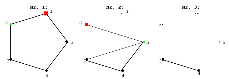
Although this result was already known for a few years Gottesman99, only very recently, such classical simulator was implemented Aaronson04 that actually requires only ${\cal O}(N^{2})$ elementary operations on classical computer. In the remainder of this section we will see how graph states can provide an alternative algorithm. This algorithm is based on elementary graph manipulations and was proposed and implemented in ref. Anders. Its complexity for the elementary gate operation requires ${\cal O}(d^{2})$ basic steps on a classical computer, where $d$ denotes the maximal degree of the graph representing the quantum register. This proposals is hence advantageous if this maximal degree remains comparably small to $N$ for the different register states throughout the computation.

According to sec. 2.2.1 any stabilizer state $|\mathcal{S}\rangle$ can be represented as a graph state $|G\rangle$ up to some LC-unitaries $U\in\mathcal{C}_{1}^{V}$ . Thus, in order to keep track¹⁸¹⁸ 18 Usually a stabilizer circuit is required to start in some kind of standard input state $|0\rangle^{V}$ of the computational basis, which has a trivial representation in terms of graph states, i.e., $|0\rangle^{V}=H^{V}|+\rangle^{V}$ . But the following argumentation will also hold for an arbitrary stabilizer state as the input, if one allows for a polynomial overhead at the beginning of classical simulation in order to determine the corresponding graphical representation. of the different steps $i=1,\ldots,M$ in the stabilizer circuit computation, one has to store a local Clifford unitary $W_{i}$ as well as the graph $G_{i}$ of the graph state $|G_{i}\rangle$ , which is LC-equivalent to the actual stabilizer state $|\mathcal{S}_{i}\rangle$ in the quantum register of step $i$ , i.e., $|\mathcal{S}_{i}\rangle=W_{i}|G_{i}\rangle$ . Note that the storage of a graph $G_{i}$ on $N$ vertices requires only $\frac{N(N-1)}{2}$ bits for the entries of the corresponding adjacency matrix. Moreover as discussed in sec. 2.2.1 at each vertex $a$ the list of single-qubit LC-unitaries $W_{i}$ can be characterized by one of $24$ ‘permutations’ $W_{i}^{a}$ of the Pauli matrices depicted in Table 1.

In order to be an efficient representation for the classical simulation of the stabilizer circuit, the graphical description remains to be provided with a set of graphical rules that account for the changes of the stabilizer when a one- or two-qubit gate or some single-qubit Pauli measurement is applied to it. The one-qubit Clifford unitary occurring at a vertex can easily be dealt with by updating the corresponding unitary according to some fixed ‘multiplication table’. For the two-qubit unitaries we will, instead of the CNOT gate, consider the phase gate $U_{ab}$ in eq. 22, since on ‘pure’ graph states it simply acts by adding or deleting the corresponding edge $\{a,b\}$ . However, the case where $U_{ab}$ does not act directly on $|G\rangle$ but on $W|G\rangle$ for some LC-unitary $W$ that is non-trivial at the vertices $a$ and $b$ , i.e., $W^{a}\neq\mathbf{1}_{a}$ or $W^{b}\neq\mathbf{1}_{b}$ , requires a more careful treatment. Remember that each of the possible single-qubit unitaries has a decomposition in terms of elementary $\frac{\pi}{4}$ –rotations given in Table 1. Since all unitaries $W_{a}=\mathbf{1}_{a},z^{a},x^{a},y^{a},\sqrt{\pm i\sigma_{z}}$ can be ‘commuted through’ the phase gate yielding at most some additional $\sigma_{z}$ on the vertex $a$ or $b$ , e.g. $U_{ab}\sigma_{x}^{a}=\sigma_{x}^{a}\sigma_{z}^{b}U_{ab}$ , we are left with the analysis of the $14$ additional cases, for which at least one unitary $W_{a}$ or $W_{b}$ is of the type $\sqrt{\pm i\sigma_{x}}$ or $\sqrt{\pm i\sigma_{y}}$ . The graphical rules for these cases can be obtained using the LC-rule derived in sec. 2.2.2 in order to remove these unitaries. For example, one finds that for an arbitrary graph $G$

U_{ab}\,\sqrt{\pm i\sigma_{x}}^{a}|G\rangle=\sqrt{\mp i\sigma_{z}}^{N_{a}}\,U_{ab}|\tau(G)\rangle\;,

(95)

since $\sqrt{+i\sigma_{x}}^{a}=\sqrt{-i\sigma_{z}}^{N_{a}}(U^{\tau}_{a})^{\dagger}$ (similarly for $\sqrt{-i\sigma_{x}}^{a}$ ), where $U^{\tau}_{a}$ denotes the LC-unitary in eq. (43) for the LC-rule. In fact in ref. Anders it is shown that, in this way, any of the remaining LC-unitaries $W_{a}$ at some vertex $a$ can be removed by means of at most five local complementations $\tau$ applied at this vertex or at one of its neighbors.

P_{x,\pm}\sigma_{z}=\sigma_{z}P_{x,\mp}

P_{y,\pm}\sigma_{z}=\sigma_{z}P_{y,\mp},

P_{z,\pm}\sigma_{z}=\sigma_{z}P_{z,\pm},

P_{x,\pm}(-i\sigma_{z})^{1/2}=(-i\sigma_{z})^{1/2}P_{y,\mp},

P_{x,\pm}(i\sigma_{y})^{1/2}=(i\sigma_{y})^{1/2}P_{z,\pm}

P_{x,\pm}(-i\sigma_{y})^{1/2}=(-i\sigma_{y})^{1/2}P_{z,\pm}

P_{x,\pm}(i\sigma_{z})^{1/2}=(i\sigma_{z})^{1/2}P_{y,\pm},

P_{y,\pm}(-i\sigma_{z})^{1/2}=(-i\sigma_{z})^{1/2}P_{x,\pm},

P_{y,\pm}(i\sigma_{y})^{1/2}=(i\sigma_{y})^{1/2}P_{y,\pm},

P_{y,\pm}(-i\sigma_{y})^{1/2}=(-i\sigma_{y})^{1/2}P_{y,\pm},

P_{y,\pm}(i\sigma_{z})^{1/2}=(i\sigma_{z})^{1/2}P_{x,\mp},

P_{z,\pm}(-i\sigma_{z})^{1/2}=(-i\sigma_{z})^{1/2}P_{z,\pm},

P_{z,\pm}(i\sigma_{y})^{1/2}=(i\sigma_{y})^{1/2}P_{x,\pm},

P_{z,\pm}(-i\sigma_{y})^{1/2}=(-i\sigma_{y})^{1/2}P_{x,\pm},

P_{z,\pm}(i\sigma_{z})^{1/2}=(i\sigma_{z})^{1/2}P_{z,\pm},

Table 2: The relevant commutation relations for Pauli projections and Clifford operators if a sequence of Pauli measurements is applied to a graph state.

Let us finally examine the effect of single-qubit Pauli measurements in more detail, since the graphical rules will be used in the subsequent secs. We will at first consider the case of a projective measurement of some Pauli operator $\sigma_{x}$ , $\sigma_{y}$ or $\sigma_{z}$ at a singe vertex $a$ in a graph state without additional LC-unitaries at this vertex and will later mention how to cope with the general case. For a Pauli measurement of the graph state $|G\rangle$ at a vertex $a$ we find that the graph $|G^{\prime}\rangle$ on the remaining unmeasured vertices can be obtained from the initial graph $G$ by means of vertex deletion and local complementation:

$\sigma_{z}:$: deleting the vertex $a$ from $G$ ;
$\sigma_{y}:$: inverting $G[N_{a}]$ and deleting $a$ ;
$\sigma_{x}:$: choosing any $b_{0}\in N_{a}$ , inverting $G[N_{b_{0}}]$ , applying the rule for $\sigma_{y}$ and finally inverting $\tilde{G}[N_{b_{0}}]$ again.

This is the content of the following proposition He04, schlinge04.

Proposition 7 (Local Pauli measurements)

A projective measurement of $\sigma_{x}$ , $\sigma_{y}$ , or $\sigma_{z}$ on the qubit associated with a vertex $a$ in a graph $G$ yields up to local unitaries $U_{i,\pm}^{a}$ a new graph state $|G^{\prime}\rangle$ on the remaining vertices. The resulting graph $G^{\prime}$ is

$\displaystyle P^{a}_{z,\pm}\|G\rangle$	$\displaystyle=$	$\displaystyle\frac{1}{\sqrt{2}}\,\|z,\pm\rangle^{a}\otimes U_{z,\pm}^{a}\|G-a\rangle,$	(96)
$\displaystyle P^{a}_{y,\pm}\|G\rangle$	$\displaystyle=$	$\displaystyle\frac{1}{\sqrt{2}}\,\|y,\pm\rangle^{a}\otimes U_{y,\pm}^{a}\|\tau_{a}(G)-a\rangle,$	(97)
$\displaystyle P^{a}_{x,\pm}\|G\rangle$	$\displaystyle=$	$\displaystyle\frac{1}{\sqrt{2}}\,\|x,\pm\rangle^{a}\otimes U_{x,\pm}^{a}\|\tau_{b_{0}}\left(\tau_{a}\circ\tau_{b_{0}}(G)-a\right)\rangle\,,$	(98)

for any choice of some $b_{0}\in N_{a}$ , whenever the $\sigma_{x}$ -measurement is not performed at an isolated vertex. If $a$ is an isolated vertex, then the outcome of the $\sigma_{x}^{a}$ -measurement is $+1$ , and the state is left unchanged. The local unitaries $U_{i,\pm}^{a}$ are

$\displaystyle U_{z,+}^{a}=$	$\displaystyle\mathbf{1},$	$\displaystyle U_{z,-}^{a}=\sigma_{z}^{N_{a}},$	(99)
$\displaystyle U_{y,+}^{a}=$	$\displaystyle\sqrt{-i\sigma_{z}}^{N_{a}},$	$\displaystyle U_{y,-}^{a}=\sqrt{+i\sigma_{z}}^{N_{a}}$	(100)
$\displaystyle U_{x,+}^{a}=$	$\displaystyle\sqrt{+i\sigma_{y}}^{b_{0}}\sigma_{z}^{N_{a}\setminus(N_{b_{0}}\cup b_{0})},$	$\displaystyle U_{x,-}^{a}=\sqrt{-i\sigma_{y}}^{b_{0}}\sigma_{z}^{N_{b_{0}}\setminus(N_{a}\cup a)}.$	(101)

For a measurement of $\sigma_{x}$ the local unitary $U_{x,\pm}$ depends on the choice of $b_{0}$ . But the resulting graph states arising from different choices of $b_{0}$ and $b^{\prime}_{0}$ will be equivalent via the LC-unitary $U_{b^{\prime}_{0}}U^{\dagger}_{b_{0}}\in\mathcal{C}_{1}^{V}$ .

For a sequence of local Pauli measurements, the local unitaries have to be taken into account, if the measured qubit is affected by the unitary. We have summarized the necessary commutation relations in Table 2, which denote the transformation of the measurement basis, if a subsequent measurement is applied to a unitarily transformed graph state. Fig. 8 shows two subsequent applications of the rather complicated $\sigma_{x}$ -measurement. An exhaustive table can also be provided for the general case that the Pauli measurement occurs at some vertex $a$ that has an arbitrary non-trivial LC-unitary $W_{a}$ attached to it.

Proof (of Proposition 7): The $\sigma_{z}$ -measurement rule follows directly from the definition of graph states in terms of the underlying interaction pattern (see eq. (24)):

$\displaystyle P_{z,\pm}^{a}\|G\rangle$	$\displaystyle=$	$\displaystyle P_{z,\pm}^{a}\prod_{\{a,b\}\in E}U_{ab}\prod_{\genfrac{}{}{0.0pt}{}{\{c,d\} \in E}{c,d \neq a}}U_{cd}\|+\rangle^{V}$	(102)
	$\displaystyle=$	$\displaystyle P_{z,\pm}^{a}\,\left(P_{z,+}^{a}+P_{z,-}^{a}\sigma_{z}^{N_{a}}\right)\,\|+\rangle^{a}\otimes\|G\setminus a\rangle^{V\setminus a}$
	$\displaystyle=$	$\displaystyle\frac{1}{\sqrt{2}}\,\left\{\begin{array}[]{ll}\|z,+\rangle^{a}\otimes\|G\setminus a\rangle^{V\setminus a}&\text{\small if measurement result is}\;m_{z}^{a}=+1\\ \|z,-\rangle^{a}\otimes\sigma_{z}^{N_{a}}\|G\setminus a\rangle^{V\setminus a}&\text{\small if measurement result is}\;m_{z}^{a}=-1\end{array}\right.$

In other words, with probability $\tfrac{1}{2}$ a $\sigma_{z}$ -measurement at a vertex of some graph state gives either $|G\setminus a\rangle$ as the graph state on the remaining vertices if the measurement outcome is $m_{z}=+1$ or $\sigma_{z}^{N_{a}}|G\setminus a\rangle$ as the graph state on the remaining vertices if the measurement outcome is $m_{z}=-1$ .

With the LC-rule at hand (see Proposition 5) one can now derive the measurement rules for a $\sigma_{x}$ - or $\sigma_{y}$ -measurement from this $\sigma_{z}$ -measurement rule. For this, one can use commutation relations, which are similar to those in Table 2, in order to show that

	$\displaystyle P^{a}_{x,\pm}$	$\displaystyle=$	$\displaystyle U^{\tau}_{b_{0}}(G)P^{a}_{y,\pm}(U^{\tau}_{b_{0}}(G))^{\dagger}$		(106)
	$\displaystyle P^{a}_{y,\pm}$	$\displaystyle=$	$\displaystyle U^{\tau}_{a}(G)P^{a}_{z,\mp}(U^{\tau}_{a}(G))^{\dagger}\,$		(107)

where $b_{0}$ is a neighbor¹⁹¹⁹ 19 Note that if $a$ is an isolated vertex the graph state is $|G\rangle=|+\rangle^{a}\otimes|G^{\prime}\rangle^{V\setminus a}$ for some graph on the remaining vertices. In this case a $\sigma_{x}$ -measurement yields $+1$ with probability $1$ . of $a$ in $G$ . With eq. (107) and using $e^{\pm i\frac{\pi}{4}\sigma_{k}}=\sqrt{\pm i\sigma_{k}}=\frac{\mathbf{1}\pm i\sigma_{k}}{\sqrt{2}}$ we can now compute

$\displaystyle P^{a}_{y,\pm}\|G\rangle$	$\displaystyle=$	$\displaystyle U^{\tau}_{a}(G)P^{a}_{z,\mp}\|\tau_{a}(G)\rangle$
	$\displaystyle=$	$\displaystyle U^{\tau}_{a}(G)\frac{1}{\sqrt{2}}\,\left\{\begin{array}[]{ll}\|z,-\rangle^{a}\otimes\sigma_{z}^{N_{a}}\|\tau_{a}(G)\setminus a\rangle^{V\setminus a}&\text{\small if }\;m_{y}^{a}=+1\\ \|z,+\rangle^{a}\otimes\|\tau_{a}(G)\setminus a\rangle^{V\setminus a}&\text{\small if}\;m_{y}^{a}=-1\end{array}\right.$
	$\displaystyle=$	$\displaystyle\frac{1}{\sqrt{2}}\,\left\{\begin{array}[]{ll}\sqrt{-i\sigma_{x}^{a}}\|z,-\rangle^{a}\otimes\sqrt{i\sigma_{z}^{N_{a}}}\sigma_{z}^{N_{a}}\|\tau_{a}(G)\setminus a\rangle^{V\setminus a}&\text{\small if }\;m_{y}^{a}=+1\\ \sqrt{-i\sigma_{x}^{a}}\|z,+\rangle^{a}\otimes\sqrt{i\sigma_{z}^{N_{a}}}\|\tau_{a}(G)\setminus a\rangle^{V\setminus a}&\text{\small if }\;m_{y}^{a}=-1\end{array}\right.$
	$\displaystyle\propto$	$\displaystyle\frac{1}{\sqrt{2}}\,\left\{\begin{array}[]{ll}\|y,+\rangle^{a}\otimes\sqrt{-i\sigma_{z}^{N_{a}}}\|\tau_{a}(G)\setminus a\rangle^{V\setminus a}&\text{\small if }\;m_{y}^{a}=+1\\ \|y,-\rangle^{a}\otimes\sqrt{i\sigma_{z}^{N_{a}}}\|\tau_{a}(G)\setminus a\rangle^{V\setminus a}&\text{\small if }\;m_{y}^{a}=-1\end{array}\right.$

This is the $\sigma_{y}$ -measurement rule, from which the $\sigma_{x}$ -measurement rule now can be derived along the same lines using eq. (106).

4 Examples and applications

In this section we give some prominent, not necessarily distinct classes of examples for graph states. We also sketch important applications of these states in multi-party quantum communication, quantum computation and quantum error correction. These examples illustrate that graph states do not only provide an interesting model to study multi-party entanglement, as it will be carried out in the following sections, but can also be an important resource for quantum information processing.

4.1 GHZ–states

Figure 9: The GHZ-state is LU-equivalent to the graph state corresponding to a star graph or the complete graph.

We start by considering the $N$ --qubit Greenberger-Horne-Zeilinger states

|GHZ\rangle=\frac{1}{\sqrt{2}}(|0\rangle^{\otimes N}+|1\rangle^{\otimes N}),

(117)

which were introduced in ref. GHZ89 for the case of three qubits and since serve as a ‘text book’ example for multi-party entangled ‘Schrödinger cat’ states. These states are special examples of states that maximally violate multi-partite Bell inequalities BI and can, for instance, be used to improve frequency standards Frequency. GHZ states have also become an interesting resource for multi-party quantum communication, e.g. in the context of secret sharing and secure function evaluation Secure. The multi--party GHZ-state corresponds to the star graph and the complete graph. This is easily seen by applying Hadamard unitaries $H^{V\setminus a}$ to all but one qubit $a$ in the GHZ-state, which yields the star graph state with $a$ as the central qubit. A further application of the LC-unitary $U_{a}^{\tau}$ for the LC-rule $\tau_{a}$ in Proposition 5 then transforms the star graph state into the complete graph state. Thus the star graphs for different central vertices as well as the complete graph are LC-equivalent representations of the GHZ-state.

4.2 Cluster states and the one-way quantum computer

The initial resource for quantum computation in the one-way quantum computer ( $\text{QC}_{G}$ ), as it was introduced in refs. Briegel01, OneWay1, OneWay2, OneWay3, OneWay5, is the cluster state in two dimensions, which corresponds to a rectangular lattice. More generally, a $d$ -dimensional cluster state is represented by a graph of the form of a $d$ -dimensional lattice. But only cluster states of dimension two and higher can serve as a universal resource for quantum computation Nielsen05a.

In the following we consider the example of the quantum Fourier transform (QFT) on three qubits as depicted in fig. 10 to sketch the basic concept of the $\text{QC}_{G}$ model. In the standard framework of quantum computation²⁰²⁰ 20 For details we refer e.g. to ref. NielsenBook. this QFT is implemented by performing a sequence of elementary ( $2$ -qubit) gates operating on the $n=3$ input qubits. In the $\text{QC}_{G}$ model we start instead with the preparation of a highly entangled resource state via the same entangling procedure as for the cluster state, except that a subset of $n$ of these qubits representing the input qubits initially are prepared in the desired input state. Then the actual computation consists in a sequence of local measurements which turns the state on the remaining, non-measured qubits into the desired (pure) output state.

In general, the measurement outcomes of the local measurements have to be stored in a classical register (’information flow vector’) of $2n$ bits, since the direction of subsequent measurements have to be adapted according to these results OneWay1, OneWay2, OneWay3, OneWay5. Moreover, each measurement round requires an update of the information flow vector that contains the ‘algorithmic information’, from which, at the end, the outcome of the quantum computation²¹²¹ 21 E.g. as it would have been obtained by a corresponding network of quantum gates. can be read off directly. The different dependencies of the measurement directions upon previous measurement results induce a temporal ordering on the set of vertices that can be measured simultaneously, whose total length represent the temporal complexity of the quantum computation in the $\text{QC}_{G}$ model. In a first measurement round all Pauli-measurements can be performed at the same time, since these do not depend on previous measurement results. This fraction of the quantum computation corresponds to the part of the network model that solely consists of Clifford operations. According to the Gottesmann-Knill theorem²²²² 22 See Proposition 6 in sec. 3. this Clifford part can be efficiently simulated on a classical computer. Note that stabilizer circuits are not even universal for classical computation Aaronson04.

In the framework of the $\text{QC}_{G}$ the stabilizer circuits can be dealt with by using only a single measurement round. If the input state is some stabilizer state, e.g. some state of the computational basis, then such a Pauli-measurement round still ends up in a stabilizer state, whereas the states obtained after some subsequent measurements can in general no longer be described within the stabilizer formalism. Note that the first measurement round might as well contain the input and output²³²³ 23 If the objective of the quantum computation is not only to compute a (coherent) quantum state on the output qubits but also to perform a read out in order to obtain some classical result. vertices, which in general are measured in $\sigma_{x}$ - and $\sigma_{z}$ -direction if the quantum computation is carried out with respect to the computational basis. In other words, input and output qubits can also be measured long before the whole quantum computation is completed, since then the actual result of the quantum computation is given by the information flow vector after the last measurement round.

In fig. 10 we have depicted the graphs that are obtained after performing all $\sigma_{z}$ measurements and after all Pauli measurements except those at the input and output vertices. The corresponding graph states can still be used to implement the QFT. For this the input state is teleported²⁴²⁴ 24 Note that this teleportation can be described within the $\text{QC}_{G}$ picture. For this the qubit holding the input state at qubit $a_{1}$ , some auxiliary qubit $a_{2}$ in the $|+\rangle$ state and the qubit at the input vertex $b$ are entangled to form a chain attached to the graph at $b$ . Then $a_{1}$ and $a_{2}$ are measured in $\sigma_{x}$ -direction. The resulting state on the graph vertices now coincides with the state after some teleportation of the input state into the vertex $b$ (up to LC). into the input vertices and the usual measurement protocol is applied. Alternatively one can regard the graph as a preparation procedure for an initial resource that already incorporates the input state. More precisely one prepares the input qubits in the input state and the remaining qubits in the $|+\rangle$ state, entangles the qubits according to the interaction pattern given by the graph and finally carries out the measurement protocol as described above.

In OneWay1, OneWay2, OneWay3, OneWay5 it is shown that any quantum algorithm within the network picture requiring only a polynomial²⁵²⁵ 25 In $n$ input qubits. amount of temporal, spatial and operational resources can be efficiently simulated by a $\text{QC}_{G}$ that requires (i) a polynomially overhead of elementary operations in the classical preprocessing to derive the equivalent setup and measurement protocol for the $\text{QC}_{G}$ , (ii) a polynomially bounded amount of classical and quantum resources, and finally (iii) a polynomial increasing time cost for the classical and quantum processing during the computation²⁶²⁶ 26 The complexity of the quantum processing is given by the number of local measurements. For the classical processing the number of elementary classical steps for the update of the information flow vector and for the determination of subsequent measurement directions is logarithmic in $n$ and proportional to the number of measurement rounds.. In this way the $\text{QC}_{G}$ can serve as a universal model for quantum computation that has quite promising scaling behavior for those practical implementations, in which the resource cluster state or more generally the initial graph state can be prepared by a homogeneous Ising interaction, i.e., independently of the system size. Furthermore, the $\text{QC}_{G}$ is equivalent Ve04, 1QCequiv to other measurement-based schemes for quantum computations.

First results towards fault-tolerant quantum computation with the $\text{QC}_{G}$ were also obtained in refs. OneWay1, OneWay2, OneWay3, OneWay5. For a reasonable noise model, including noisy cluster state preparation as well as erroneous measurements, a quantum computation subjected to decoherence below a certain threshold can be implemented on a $\text{QC}_{G}$ in a fault-tolerant way. This means that for sufficiently small noise of a specific type the quantum computation can be implemented on a $\text{QC}_{G}$ with ‘any’ desired accuracy if one allows for a reasonable overhead in the computational resources. But note that the derived error threshold seems rather unrealistic for practical purposes. Current research focuses on an improvement of this threshold and a generalization of the underlying noise model combining standard concepts of quantum error correction with some intrinsic error detection possibilities of the $\text{QC}_{G}$ and purification methods for the underlying graph state as the computational resource (see sec. 4.4). Further results on fault tolerant quantum computation can also be found in ref. FaultTolOneWay.

4.3 Quantum error correcting codes

For quantum error correcting codes based on stabilizer codes Gottesman the codewords as well as the encoding procedures can be represented as graphs Schlinge02a, Schlinge02b, Grassl02. The latter can be understood along the lines of the previous subsection, because the graph state is the computational resource for implementing the encoding process in terms of the $\text{QC}_{G}$ model. The graphs depicted in fig. 11 for example correspond to the encoding procedures for the five-qubit Steane code and the concatenated $[7,1,3]$ -CSS-code that encode a state on one qubit into some state on five and $49$ qubits respectively.

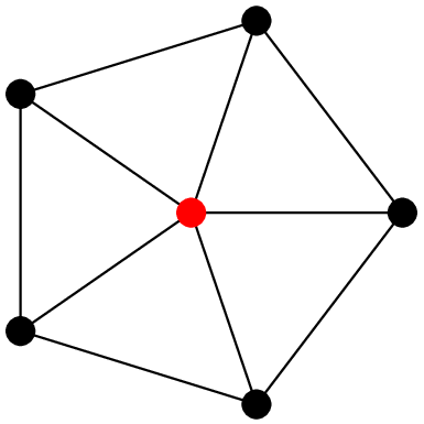
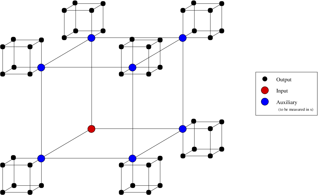
The encoding consists in preparing the qubit at the (red) input vertex in the input state and the remaining qubits in the $|+\rangle$ state, entangling the qubits according to the graph and finally measuring the (blue) auxiliary vertices²⁷²⁷ 27 Whereas the five-qubit code does not require any auxiliary qubits to be measured, the auxiliary vertices of concatenated CSS-code are located at the corners of the inner cube, where the open side indicates the input qubit. and the input vertex in the $\sigma_{x}$ -direction. In this way the input state is encoded into the state on the remaining (black) qubits. Alternatively one might as well prepare the graph states depicted in the figures as such, teleport the input state into the input vertex and then perform the same measurement protocol.

When applying this procedure to an eigenstate of one of the Pauli-matrices $\sigma_{x}$ , $\sigma_{y}$ or $\sigma_{z}$ , the encoded state is a graph state and can be regarded as a code word vector for the respective quantum code (see sec. 2.2.1). Note that the $[7,1,3]$ -CSS-code is a concatenation of the Steane code depicted in fig. 12. This means that each of the $7$ output qubits of the first encoding level is encoded again by the same encoding procedure, such that the overall encoding procedure maps some input state into an encoded state on the $7\times 7=49$ output qubits of the second level. This is graphically reflected by the fact that the right graph in fig. 11 is obtained from the left graph in fig. 12 by attaching another cube at each ‘output’-corner in the initial cube and merging the former output and input vertex into one auxiliary vertex.

4.4 CSS–states and secret sharing

The class of CSS states corresponds to the class of two-colorable graphs, i.e., graphs that allow for a coloring of the vertices with two colors such that no two adjacent vertices have the same color (see sec. 1.2). In general a CSS-code is a stabilizer code, whose stabilizer can be generated by stabilizer elements $\sigma$ that either consists of $\sigma_{x}$ - or $\sigma_{z}$ -matrices, i.e., $\sigma=\sigma_{x}^{U}$ or $\sigma=\sigma_{z}^{U}$ . By performing Hadamard operation to the vertices of one coloring partition any two-colorable graph state is easily seen to be of CSS-type²⁸²⁸ 28 I.e., a CSS code with stabilizer of full rank $\text{rank}(\mathcal{S})=N$ .. Conversely it is shown in ref. Lo04 that any CSS-state is also LC-equivalent to some two-colorable graph state.

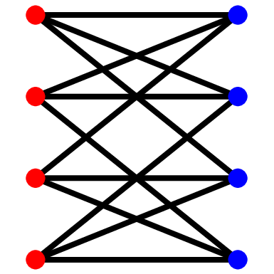
In Lo04 CSS states are used to design a ‘prepare and measure’ protocol for quantum cryptography that can be used for conference key agreement²⁹²⁹ 29 This protocol allows several parties to share a secure conference key in the presence of an eavesdropper. and quantum sharing of classical secrets³⁰³⁰ 30 This protocol allows a party to share a classical secret with $n$ parties, such that at least k other parties are needed to reveal this key (for some fixed $k>\frac{n}{2}$ )..

We remark that not all Pauli measurements preserve the two-colorability of the underlying graph. Whereas local $\sigma_{x}$ - or $\sigma_{z}$ -measurements in two-colorable graphs yield graph states according to two-colorable graphs, $\sigma_{y}$ -measurements of two-colorable graphs can lead to graph states which are not even locally equivalent to two-colorable graphs He04. This might be important in the context of 1-way QC models, in particular in the context of fault tolerance. There, graph states corresponding to the non--clifford part of a computation may be purified via multi-particle entanglement purification, where current protocols require two--colorability of the underlying graph.

4.5 Entanglement purification and secure state distribution

Despite of their central use for quantum information processing purposes, in reality, multi-partite entangled pure states, such as graph states, will not be available with unit fidelity. The reasons for this are manifold. For instance, the operations to create these states are always noisy, the distribution of these states among distant parties occurs through noisy quantum channels, and the storage of states is subjected to decoherence. For the class of two-colorable graph states entanglement purification procedures are known to maintain or purify these states. Some of these procedures Du03a provably apply to the regime of noisy control operations. The basic idea in entanglement purification is to use several copies of low-fidelity entangled states in order to distill a few highly entangled states. Thereby, one copy of the state with low fidelity is measured in order to reveal information about either one copy (recurrence and pumping schemes) or several other copies (hashing protocols) of the imperfect graph state. For the purification step each of the imperfect copies (mixed states) is transformed³¹³¹ 31 This purification is done by means of some local twirling operations (see Proposition 23 in sec. 10), so with respect to the average with respect to an appropriate local symmetry group. into a mixed state that is diagonal in a graph state basis associated with the two-colorable graph state in question. Given that the initial fidelity is sufficiently high, an ensemble of these graph diagonal states can then be purified. In Du03a genuine multi-party entanglement purification protocols based on a recurrence or pumping schemes and based on hashing procedures (see also Lo04) were considered and compared with procedures using bi-partite purification³²³² 32 Here one e.g. establishes some highly entangled pairs shared between different parties, in order to teleport the desired $N$ -particle state prepared at one party to the remaining parties.. The different purification schemes have their own advantages. But for local noise, multi-party purification protocols are, in most cases, not only more efficient but provide also better achievable fidelities for the distilled states in the case of noisy control operations. For practical purposes it is useful that the purification regime³³³³ 33 I.e., the purification regime is given by the necessary fidelity of the initial low-entangled copies, such that some higher-entangled state can be distilled. for the recurrence protocols as well as the error threshold for the noisy control operations involved seem not to depend on the number of particles in the graph state but rather on the maximal degree of the underlying graph. Thus two-colorable graph states provide a reservoir of entangled states between a large number of particles, which can be created and maintained even in the presence of decoherence. Entanglement purification schemes will be discussed in more detail in sec. 10.2.

These purification schemes were also modified to blind purification protocols. That is, the purification takes place in such a way that even the involved parties (except of a central party) do neither know the identity of the state they are attempting to purify nor have a possibility to learn it. Such protocols allow for the secure distribution of two-colorable graph states, which remain unknown to the different parties and any potential eavesdropper Du05c. Such secure state distribution is a quantum primitive in a real–world scenario (i.e., taking imperfections in local control operations and channel noise into account) which may be used as a basic building block for both quantum and classical security applications.

5 Physical implementations

Let us briefly discuss a few proposals of how to prepare graph states in real physical systems, aiming at realizing some of the applications, such as the one-way quantum computer ( $\text{QC}_{G}$ ). In general, graph states do not appear as ground states of physical systems, since, in most cases, they rely dominantly on two-body interactions Nielsen05a. Following the preparation procedure in sec. 2.1, graph states can nevertheless be obtained in any physical system that allows to implement an Ising interaction $H_{ab}^{I}=\sigma_{z}^{a}\sigma_{z}^{b}$ . In particular, graph states can be generated, of course, in all physical devices for universal quantum computation. Clearly, the complexity of the graph state preparation depends on the respective computational primitives of the physical realization Perdrix.

One may distinguish two classes of physical systems where cluster or graph state preparation very naturally reflects the underlying architecture. The first one consists in lattice systems, such as cold atoms in optical lattices. Here, a neighborhood relation is inherited by the physical neighborhood of constituents in the lattice itself, and by means of appropriate switching of interactions, one can generate cluster states of some dimension Briegel-HaenschBand. The second one comprises of physical systems where the neighborhood relation can be freely chosen, such as in purely optical systems or hybrid setups making use of ‘flying’ optical qubits for the entangling process and ‘static’ matter qubits for storage of the actual graph state. We will briefly sketch both approaches, starting with the former.

The preparation of a two- or three-dimensional cluster state (of ‘arbitrary’ size) can be regarded as a fixed operational step, if the Ising interaction can be implemented homogeneously (for all directions) throughout the whole lattice Briegel01, Briegel-HaenschBand. This globally tunable Ising interaction can be realized in optical lattices with ultra-cold atoms via state-selective displacement of the atoms and controlled cold collisions Jaksch99 or via tunneling Duan03. For instance, employing a superfluid-Mott insulation quantum phase transition a Bose-Einstein condensate can be loaded into an optical lattice achieving almost unit occupation per lattice site Jaksch98, Greiner02. Interference experiments Greiner03 indicate that graph states can be obtained within such setups. Graph states prepared in optical lattices therefore are a promising resource for scalable quantum computation in the framework of the one-way quantum computer, since cluster states can be created with an operational effort that is independent of the system size. Existing implementations are currently still facing at least two major challenges: On one hand, the number of atoms at each lattice site has to be exactly controllable. In particular, the presence of defects, i.e., empty lattice sites, might spoil any quantum computation. On the other hand, the one-way computer requires the atoms at different sites to be individually addressable by local measurements. A number of proposals have already been made to overcome these obstacles (see, e.g., refs. Kay05, Vollbrecht04, Rabl03), and one can say that optical lattices remain one of the prime candidates to study multi-particle entanglement and scalable quantum computation. Alternative implementations have also been suggested for physical systems, in which the underlying Hamiltonian is given by an (isotropic) Heisenberg interaction Clark04, Loss05. These proposals can be realized in XY-spin chains formed within an optical lattice of neutral atoms as well as in solid-state systems, such as quantum dots.

The second type of physical systems does not directly exploit immediate adjacency of the respective constituents: In this class of physical systems the key point is the fact that one introduces a separation between the act of creating entanglement and the act of performing the actual computation. This is of central importance in particular in setups where the elementary gates function on a probabilistic basis, or where erasure errors such as photon losses constitute the predominant obstacle that has to be overcome. This very much applies to architectures of quantum computing based on linear optics. Linear optical setups are attractive, as photons are relatively robust with respect to decoherence, and accurate state control is possible using linear optical elements KLM. However, in order to achieve universal quantum computing based on dual rail encoding – where logical qubits are encoded in state vectors $|0\rangle|1\rangle$ and $|1\rangle|0\rangle$ of two modes – measurements are necessary, rendering any scheme probabilistic. Notably, the scheme of Knill, Laflamme, and Milburn in ref. KLM employs the non-linear sign shift gate, acting as

x_{0}|0\rangle+x_{1}|1\rangle+x_{2}|2\rangle\mapsto x_{0}|0\rangle+x_{1}|1\rangle-x_{2}|2\rangle

(118)

as a primitive probabilistic gate, realized using additional modes and measurement. Here, $|0\rangle$ , $|1\rangle$ , and $|2\rangle$ denote the state vectors of states containing $0,1,2$ photons. It has been shown that, although these gates operate on a probabilistic basis (only certain measurement outcomes are accepted as being successful), the overall computational scheme can be uplifted to almost unit success probability. This is done using teleportation, based on appropriate entangled resources which are in turn built up by invoking these probabilistic gates. This is a powerful theoretical idea, heavily exploiting the previously described stabilizer formalism. So in this way, near-deterministic quantum computation is possible in principle using linear optical elements, single-photon sources, photon-resolving detectors, and feedforward, meaning later action may depend on earlier measurement outcomes KLM. Practically, the key obstacle is, however, that the required resources are tremendous (approximately $10^{5}$ beam splitters required for a single CNOT gate operating with a failure rate of $10^{-4}$ ), essentially originating from the fact that the elementary gates work with such a small probability of success NSBound.

Graph state methods can indeed significantly reduce the surmounting number of required resources (although still giving rise to challenging prescriptions). In the remainder of this section, we will thus briefly review recent work discussing graph states and one-way quantum computation in the context of linear optical setups. Ref. Reznik is the first work making use of states related to graph states to reduce the overhead in resources. In ref. Nielsen04, the presented scheme has explicitly been phrased in terms of cluster and graph states, making use of the setting of the scheme by Knill-Laflamme-Milburn.

The number or necessary resources was further reduced in refs. Browne04, Ralph05, employing two types of fusing gates that glue pieces of linear one-dimensional clusters or of two-dimensional graph states together. Essentially, the basic resource here are Bell states using non-deterministic parity-check measurements PC, involving the combination of photons on polarizing beam splitters, followed by measurements on the output modes. The computational basis is again the one of dual rail encoding, here specifically the basis

|{H}\rangle:=|0\rangle|1\rangle,\,\,\,\,|{V}\rangle:=|1\rangle|0\rangle

(119)

corresponding to a horizontally and vertically polarized photon. A fusion of the first type amounts to mixing the input, assumed to contain only one photon per spatial mode, at a polarizing beam splitter, rotating the output by $45^{o}$ and measuring it with a polarization-discriminating photon detector. This is the parity-check operation considered in ref. PC. In the case when one and only one photon is detected – occurring with a probability of $1/2$ and considered the successful event – the state is transformed according to a non-trace-preserving completely positive maps with either of the two Kraus operators,

	$\displaystyle K_{1}$	$\displaystyle=$	$\displaystyle\left(\|{H}\rangle\langle{H}\|\langle{H}\|-\|{V}\rangle\langle{V}\|\langle{V}\|\right)/\sqrt{2},$		(120)
	$\displaystyle K_{2}$	$\displaystyle=$	$\displaystyle\left(\|{H}\rangle\langle{H}\|\langle{H}\|+\|{V}\rangle\langle{V}\|\langle{V}\|\right)/\sqrt{2}.$		(121)

Given such a successful event, one glues two pieces of a graph state together Browne04. From maximally entangled two-dimensional resources, one can build up linear cluster states. For a first experimental demonstration, see ref. Zhang05. To build up higher-dimensional structures, a variant of a destructive CNOT gate can be used PC, in ref. Browne04 referred to as fusion of second type. This fusion gate of the second type consists of a polarizing beam splitters, two polarization rotators of $45^{o}$ at the inputs and outputs each, followed again by polarization resolving photon detection. These gates are still probabilistic, yet, failures can be tolerated by merely rebuilding the affected graph section, assuming that failures are heralded, meaning that one has classical knowledge of inappropriate measurement outcomes. First steps towards fault tolerance with respect to photon losses have been taken Trees. In this way, graph states can be prepared from essentially probabilistic ingredients, giving rise to deterministic quantum computation with smaller overhead in resources.

Quite recently, arbitrary graph states on four qubits were experimentally generated in an entirely optical system, with the four qubits being represented by the polarization state of four photons Walther05. Although the feasibility of $1$ -QC was demonstrated through a set of one- and two-qubit operations, at the present stage such experiments rather constitute a proof-of-principle than a clear-cut route to scalable quantum computation. This is mainly because the scalability of the preparation by means of parametric down conversion is currently bound to only a few photons. Using such technology as source of entangled photons, hence, the overall success probability is exponentially decreasing.

An alternative route in the second framework is provided by hybrid solutions, where the advantages of photons providing coupling mechanisms and of matter systems as long-lived storage devices are simultaneously exploited. Based on schemes that allow for the preparation of entangled states using matter systems in leaking cavities using flying optical qubits flyingQubits, Cabrillo, one can immediately construct schemes that allow for graph state preparation Sean, Almut, Benjamin, even in setups where in intermediate steps no further local rotations of the state of the matter qubits is required. The matter qubits may be spatially separated, and the adjacency pattern of the graph states to be prepared is in then, in principle, completely arbitrary. Such schemes can even be made essentially deterministic, in that if an entangling operation fails, it can often be repeated until a successful operation occurs, without damage to the nascent graph state Almut, Benjamin. Using multi-port linear optical devices, the need of doing intermediate local rotations can also be largely eliminated in the preparation of the graph states. Also, whole parts of graph states can be fused together, in an essentially deterministic manner. In architectures making use of optically active electron-nuclear systems, such as in N-V-centers in diamond, one has effectively a ${\mathbbm{C}}^{2}\otimes{\mathbbm{C}}^{2}$ -system locally available, allowing for a way to entangle matter qubits in a way that is more robust with respect to unavoidable photon loss NV. All these schemes have in common that the neighborhood relation between constituents is fairly arbitrary, and that arbitrary graph states can – in principle – directly be prepared.

One general lesson to learn from graph state approaches from the perspective of implementations is that there are probably no generally valid uncompromising requirements for physical systems to allow for scalable quantum computation. Instead, it very much depends on the underlying physical architecture what computational model is advantageous; hence rendering otherwise inappropriate architectures useful and promising. Schemes for quantum computing based on graph states promise to significantly lessen the challenges posed by the obvious requirement in any scheme for quantum computation, that one needs extraordinarily good isolation against decoherence effects and precise state manipulation at the same time.

6 Reduced states of graph states

As we will discuss in sec. 8, for pure multi-partite states the reduced state obtained after tracing out (forgetting the information in) some part of the system captures many interesting entanglement properties of the state. More precisely, consider a pure state $|\psi\rangle^{AB}$ of a joint system of parties $A$ and $B$ . On the one hand the reduced state

\rho^{A}:=\text{tr}_{B}(\rho)

(122)

represents the information available for one subsystem $A$ , if it is not provided with any information that corresponds to some measurement statistics on party $B$ . The study of entanglement accessible to subsystem $A$ in this way is an interesting issue in itself. On the other hand, for pure states $\rho=|\psi\rangle\langle\psi|$ the state $|\psi\rangle$ is entangled with respect to the partitioning $(A,B)$ iff the reduced state $\rho^{A}=\text{tr}_{A}(\rho)$ is mixed and thus cannot be written as a product state $|\psi\rangle^{AB}=|\psi\rangle^{A}|\psi\rangle^{B}$ . Moreover, the mixedness of this reduced state $|\psi\rangle^{AB}$ , for example in terms of some entropic measure, allows one to quantify the amount of entanglement contained in this state between the parties $A$ and $B$ .

The following proposition shows that for graph states the reduced density matrices can be represented efficiently in terms of their stabilizer elements or their adjacency matrix He04, Nest04c.

Proposition 8 (Reduced state)

Let $A\subseteq V$ be subset of vertices for a graph $G=(V,E)$ and $B=V\setminus A$ the corresponding complement in $V$ . The reduced state $\rho^{A}_{G}:=\text{tr}_{B}\left(|G\rangle\langle G|\right)$ is given by

\rho^{A}_{G}=\frac{1}{2^{|A|}}\,\sum_{\sigma\in\mathcal{S}_{A}}\,\sigma\;,

(123)

where

S_{A}:=\{\sigma\in\mathcal{S}\,|\,\text{supp}(\sigma)\subseteq A\}

(124)

denotes the subgroup of stabilizer elements $\sigma\in\mathcal{S}$ for $|G\rangle$ with support³⁴³⁴ 34 The support of a Pauli operator $\sigma=\sigma_{i_{1}}^{1}\otimes\ldots\otimes\sigma_{i_{N}}^{N}$ is the set of all indices $a\in V$ for which $\sigma$ acts non-trivially, i.e., $i_{a}\neq 0$ . on the set of vertices within $A$ . $\rho_{G}^{A}$ is up to some factor a projection, i.e.,

\left(\rho_{G}^{A}\right)^{2}=\frac{|\mathcal{S}_{A}|}{2^{|A|}}\,\rho_{G}^{A}\;.

(125)

It projects onto the subspace in $\mathbf{H}^{A}$ spanned by the vectors

|\mathbf{\Gamma}^{\prime}B^{\prime}\rangle_{G[A]}=\sigma_{z}^{\mathbf{\Gamma}^{\prime}B^{\prime}}\,|G[A]\rangle\hskip 28.45274pt(B^{\prime}\subseteq B)\;,

(126)

where $G[A]=G\setminus B$ is the subgraph of $G$ induced by $A$ and $\mathbf{\Gamma}^{\prime}:=\mathbf{\Gamma}^{AB}$ denotes the $|A|\times|B|$ –off–diagonal sub-matrix of the adjacency matrix $\mathbf{\Gamma}$ for $G$ that represents the edges between $A$ and $B$ :

{\@index{\@indexphrase{adjacency matrix $\mathbf{\Gamma}$}}}\left(\begin{array}[]{cc}\mathbf{\Gamma}_{A}&\mathbf{\Gamma}_{AB}\\ \mathbf{\Gamma}_{AB}^{T}&\mathbf{\Gamma}_{B}\\ \end{array}\right)=\mathbf{\Gamma}\;.

(127)

In this basis, $\rho^{A}_{G}$ can be written as

\rho^{A}_{G}=\frac{1}{2^{|B|}}\,\sum_{B^{\prime}\subseteq B}\,|\mathbf{\Gamma}^{\prime}B^{\prime}\rangle_{G[A]}\langle\mathbf{\Gamma}^{\prime}B^{\prime}|\;.

(128)

Proof: Eq. (123) immediately follows from eq. (30) and the fact that the partial trace of $\sigma=\sigma_{i_{1}}^{1}\otimes\ldots\otimes\sigma_{i_{N}}^{N}\in\mathcal{S}$ can be taken successively over the different vertices in $b\in B$ and gives $\text{tr}_{b}(\sigma_{i_{b}}^{b})=2\delta_{i_{b}0}$ . $\rho_{G}^{A}$ is proportional to a projection, i.e.,

\left(\rho_{G}^{A}\right)^{2}=\frac{1}{4^{|A|}}\,\sum_{\sigma,\sigma^{\prime}\in\mathcal{S}_{A}}\,\sigma\sigma^{\prime}=\frac{|\mathcal{S}_{A}|}{4^{|A|}}\,\sum_{\sigma\in\mathcal{S}_{A}}\,\sigma=\frac{|\mathcal{S}_{A}|}{2^{|A|}}\,\rho_{G}^{A}

(129)

follows, because $\mathcal{S}_{A}$ is a subgroup of $\mathcal{S}$ . To show eq. (128), the partial trace over $B$ can be taken in the basis of $B$ given by

|B^{\prime}\rangle^{B}_{z}\equiv\bigotimes_{b\in B}|B^{\prime}_{b}\rangle^{b}_{z}:=\sigma_{x}^{B^{\prime}}|0\rangle^{B}\;.

(130)

This basis decomposition corresponds to successive local $\sigma_{z}$ -measurements of all vertices in $B$ . The set $B^{\prime}\subseteq B$ or the corresponding binary vector determines the measurement outcomes, i.e., if $b\notin B^{\prime}$ or likewise the corresponding component of the binary vector $B^{\prime}_{b}=0$ then the measurement outcome at this vertex is $+1$ and $-1$ otherwise. According to Proposition 7, after measurement of $\sigma_{z}^{b}$ the state of the remaining vertices is the graph state vector $|G\setminus b\rangle$ in the case of the outcome $+1$ , and $\sigma_{z}^{N_{b}}|G\setminus b\rangle$ if the outcome is $-1$ . This can be summarized to

\left(\sigma_{z}^{N_{b}}\right)^{B^{\prime}_{b}}|G\setminus b\rangle,

(131)

since $B^{\prime}_{b}\in\{0,1\}$ represents the measurement result $\{+1,-1\}$ . Because the subsequent measurements commute with the previous local unitaries, the final state vector according to the result $B^{\prime}=(B^{\prime}_{b})_{b\in B}\in{\mathbbm{F}}_{2}^{B}$ is

\prod_{b\in B}\left(\sigma_{z}^{N_{b}}\right)^{B^{\prime}_{b}}\,|G\setminus B\rangle^{A}\otimes|B^{\prime}\rangle_{z}^{B}\;=\;\sigma_{z}^{\left(\sum_{b\in B}N_{b}B^{\prime}_{b}\right)}\,|G[A]\rangle^{A}\otimes|B^{\prime}\rangle_{z}^{B}\;=\;\sigma_{z}^{\mathbf{\Gamma}B^{\prime}}\,|G[A]\rangle^{A}\otimes|B^{\prime}\rangle_{z}^{B}\;,

(132)

because the sum is performed modulo 2, and for all $b\in B$ the binary vector corresponding to $N_{b}$ is the $b$ -th column of the adjacency matrix $\mathbf{\Gamma}$ . Distinguishing the two parts of the adjacency matrix $\mathbf{\Gamma}_{B}$ and $\mathbf{\Gamma}_{AB}$ that correspond to edges within $B$ , and edges between $A$ and $B$ , one arrives at the state vector associated with the measurement result given by $B^{\prime}$

(-1)^{\langle B^{\prime}|\mathbf{\Gamma}_{B}B^{\prime}\rangle}\,\sigma_{z}^{\mathbf{\Gamma}_{AB}B^{\prime}}\,|G[A]\rangle^{A}\otimes|B^{\prime}\rangle^{B}_{z}\;=\;(-1)^{\langle B^{\prime}|\mathbf{\Gamma}_{B}B^{\prime}\rangle}\,|\mathbf{\Gamma}_{AB}B^{\prime}\rangle^{A}_{G[A]}\otimes|B^{\prime}\rangle^{B}_{z}\;.

(133)

Because the possible measurement results are attained with probability $1/2$ , this proves eq. (128).

7 Equivalence classes under local operations

For a characterization of the entanglement in graph states we now examine the equivalence classes under local operations. Concerning locality we restrict to the finest partitioning, i.e., each vertex $a\in V$ represents a single party and the quantum operations $\mathcal{E}$ in question are a certain subclass of the class of all completely positive maps (CPM) that are separable with respect to this finest partitioning. Since we are interested in the equivalence classes of graph states under these local operations, we can consider the situation in which a pure state $|\psi_{1}\rangle$ is mapped onto another pure state $|\psi_{2}\rangle$ by the CPM $\mathcal{E}$ with non-zero probability. It is generally quite a subtle problem to characterize the class of all transformations $\mathcal{E}$ that can be implemented by means of local operations and classical communication (LOCC), and in the following we restrict to a subclass of LOCC-protocols where $\mathcal{E}$ factors out as the tensor product of a local operator $E_{i}$ for each party:

\mathcal{E}(\rho)=E_{1}^{1}\otimes\ldots\otimes E_{N}^{N}\,\rho\,(E_{1}^{1})^{\dagger}\otimes\ldots\otimes(E_{N}^{N})^{\dagger}\;.

(134)

This means that the pure state $|\psi_{1}\rangle$ is converted (in general: stochastically) into the state $|\psi_{2}\rangle=E_{1}^{1}\otimes\ldots\otimes E_{N}^{N}\,|\psi_{1}\rangle$ . In the following we will consider three different classes of local operations, namely

•

SLOCC: invertible stochastic local operations and classical communication, i.e., the operation $E_{a}\in\text{SL}(2,\mathbb{C})$ at each qubit is an arbitrary invertible matrix; SLOCC-equivalence occurs typically with nonunit probability;
•

LU: arbitrary local unitaries, i.e. the operation $E_{a}\in\text{SU(2)}$ at each qubit is some unitary operation; LU-equivalence occurs with unit probability;
•

LC: local Clifford unitaries, i.e., the operation $E_{a}\in\mathcal{C}_{1}$ at each qubit is one of the Clifford unitaries introduced in sec. 2.2.2; LC-equivalence occurs with unit probability;

For $\text{X}\in\{\text{LC},\text{LU},\text{SLOCC}\}$ , two states $|\psi_{1}\rangle$ and $|\psi_{2}\rangle$ are called $\text{X}-$ equivalent if there exists an $\mbox{X}-$ operator $\mathbf{X}$ such that $\mathbf{X}|\psi_{2}\rangle\sim|\psi_{1}\rangle$ . We will frequently write

|\psi_{1}\rangle\longleftrightarrow_{\text{X}}|\psi_{2}\rangle

(135)

if both states are X-equivalent.

Let us first give a brief overview of entanglement classes for arbitrary states, i.e., not necessarily graph or stabilizer states. We start with the case of two $d$ -level systems, i.e., we consider bi-partite entanglement. Here the Schmidt decomposition serves as a well-known standard form, from which the conditions for different types of interconvertibility can be read off. A bi-partite state $|\psi_{1}\rangle$ can be transformed into the state $|\psi_{2}\rangle$

|\psi_{1}\rangle\longrightarrow_{\text{X}}|\psi_{2}\rangle\hskip 19.91684pt\text{for}\hskip 14.22636pt\text{X}\in\{\text{LU},\text{LOCC},\text{SLOCC}\}

(136)

by means of (i) SLOCC, (ii) LOCC or (iii) LU operations iff for the corresponding Schmidt decomposition of

|\psi_{1}\rangle^{AB}=\sum_{i=1}^{R_{1}}\lambda^{1}_{i}|i\rangle^{A}|i\rangle^{B}\hskip 19.91684pt\text{and}\hskip 19.91684pt|\psi_{2}\rangle^{AB}=\sum_{j=1}^{R_{2}}\lambda^{2}_{j}|j\rangle^{A}|j\rangle^{B}

(137)

(i) $R_{1}\geq R_{2}$ , (ii) the coefficient list $(\lambda^{1}_{i})_{i=1}^{R_{1}}$ is a majorization of $(\lambda^{2}_{j})_{j=1}^{R_{2}}$ or (iii) the coefficient list $(\lambda^{1}_{i})_{i=1}^{R_{1}}$ coincides with $(\lambda^{2}_{j})_{j=1}^{R_{2}}$ up to permutations, respectively. It follows that in the bi-partite case the SLOCC-equivalence leads to $d$ distinct equivalence classes corresponding to the different values for the Schmidt rank $R$ . On the other hand, there is an infinite number of bi-partite LU-equivalence classes, which are parameterized by the $d$ Schmidt coefficients $\lambda_{i}$ .

Moving to multi-partite entanglement, in the case of three qubits it was shown in ref. Du00b that there are $6$ orbits under SLOCC-operations. But true three-qubit entanglement is only contained in the two distinct classes represented by the GHZ-state $|GHZ\rangle$ (see sec. 4.1) and the W-state

|W\rangle=\frac{1}{\sqrt{3}}\,\left(|0,0,1\rangle+|0,1,0\rangle+|1,0,0\rangle\right)\;.

(138)

Note that all two-qubit states are SLOCC-equivalent to a two-qubit graph state corresponding to either the empty graph (product state) or connected graph (Bell state). But the W-state is an example for a pure state on three qubits that is not SLOCC-equivalent to some graph state. This is because the GHZ-state $|GHZ\rangle$ is the only ‘connected’ graph state with three vertices, as we will see below.

For $N$ -qubit systems with $N\geq 4$ the number of orbits under SLOCC-operations is infinite and is in fact specified by an exponentially increasing number of parameters. The latter scaling behavior for the number of required parameters is due to the fact that a generic orbit is specified (up to some irrelevant complex constant) by $3N$ complex parameters describing the group $\text{SL}(2,\mathbb{C})^{\otimes N}$ in question whereas a pure state on $(\mathbb{C}^{2})^{\otimes N}$ is specified by $2^{N}-1$ complex parameters (neglecting an overall complex phase). For $4$ qubits it was shown in ref. Verstraete02a that there exists a standard form for generic states under SLOCC-operations that is determined by $3$ complex parameters and $8$ further standard forms corresponding to classes of ‘degenerate’ pure states. Needless to say that the number of LU- or LC-equivalence classes necessarily has to be specified by even more parameters since the corresponding matrix groups are contained in $\text{SL}(2,\mathbb{C})$ .

In Verstraete03a it is shown that any multi-partite state can be transformed by SLOCC-operations into some standard form that is unique up to LU, while maximizing all entanglement monotones³⁵³⁵ 35 More precisely the entanglement monotones in question are linearly homogeneous positive functions of the state that remain invariant under determinant-1-SLOCC operations.. In this way the problem of deciding, whether two states are SLOCC-equivalent, can be reduced to the problem of deciding, whether the standard forms of these states are LU-equivalent. In this formalism all pure states $|\psi\rangle$ with maximally mixed single-qubit reduced density matrices

\rho_{\psi}^{a}=\text{tr}_{V\setminus a}(|\psi\rangle\langle\psi|)=\frac{1}{2}\,\mathbf{1}_{a}\hskip 28.45274pt\forall a\in V

(139)

are standard forms of this local filtering sequence and they are maximally entangled in that these states maximize all entanglement monotones.

Let us return to the question of equivalence under local operations for graph states. We start with SLOCC-equivalence. According to Proposition 8, any single-qubit reduced state $\rho_{G}^{a}$ is maximally mixed for all graph states corresponding to connected graphs. Therefore, ‘connected’ graph states are already in standard form under SLOCC in the above sense. Thus, when restricting to connected graph states all SLOCC-equivalence classes coincide with LU-equivalence classes; this property can easily be extended to the case of general (not necessarily ‘connected’) graph states by considering each connected component separately. We arrive at the following result:

Proposition 9 (SLOCC- equals LU-equivalence)

Two graph states $|G_{1}\rangle$ and $|G_{1}\rangle$ are SLOCC-equivalent iff they are LU-equivalent Nest04c:

|G_{1}\rangle\longleftrightarrow_{\text{SLOCC}}|G_{2}\rangle\hskip 5.69046pt\Longleftrightarrow\hskip 5.69046pt|G_{1}\rangle\longleftrightarrow_{\text{LU}}|G_{2}\rangle\;.

(140)

This result was first obtained in ref. Nest04c. We remark that the question whether for graph states also

|G_{1}\rangle\longleftrightarrow_{\text{LU}}|G_{2}\rangle\hskip 19.91684pt\Longrightarrow\hskip 19.91684pt|G_{1}\rangle\longleftrightarrow_{\text{LC}}|G_{2}\rangle

(141)

holds is still an open question. Note that the backward implication is trivial since the group of LC-unitaries is a proper subgroup of all LU. For a large subset³⁶³⁶ 36 A stabilizer element $\sigma\in\mathcal{S}$ with minimal support $\text{supp}(\sigma)$ , i.e., no other stabilizer element $\sigma^{\prime}\in\mathcal{S}$ has a support $\text{supp}(\sigma^{\prime})$ that is a proper subset of $\text{supp}(\sigma)$ , is called minimal element of $\mathcal{S}$ . Let $\mathcal{M}$ denote the subgroup generated by all minimal elements in $\mathcal{S}$ . Now the notion of LU- and LC-equivalence coincide for all stabilizer states, for which $\sigma_{x}$ , $\sigma_{y}$ and $\sigma_{z}$ occurs at each qubit in $\mathcal{M}$ . of graph states, however, it was shown in Nest04d that both notions of equivalence coincide. The hypothesis of a general coincidence for all graph states is further supported by results CliffordInvariants about the corresponding invariants under these operations, which will be briefly reviewed later in this section, and the classification of graph states with up to seven vertices that we will discuss below. Note that a general coincidence of SLOCC-, LU- and LC-equivalence for graph states would be particularly advantageous for the following two reasons: since in this case all 3 local equivalences would correspond to LC-equivalence, firstly, checking whether two given graph states are locally equivalent could then be done efficiently (see sec. 2.2.4); secondly, all 3 locally equivalences would entirely be described by the local complementation rule, yielding a description of local equivalence of graph states in simple, purely graph theoretic terms.

To distinguish the different equivalence classes under LU (or, equivalently, SLOCC) we will first derive a simple (though not complete) set of invariants that can be efficiently computed for graph states from the underlying adjacency matrix of the graph. As mentioned above, for any pure state $|\psi\rangle^{AB}$ in the joint system $\mathbf{H}_{A}\otimes\mathbf{H}_{B}$ of two parties $(A,B)$ with arbitrary dimensionality $d_{A}=\text{dim}_{\mathbb{C}}\mathbf{H}_{A}$ and $d_{B}=\text{dim}_{\mathbb{C}}\mathbf{H}_{B}$ the Schmidt rank³⁷³⁷ 37 Note that from the Schmidt decomposition it follows that $\text{SR'}^{A}(\psi)=\text{SR'}^{B}(\psi)$ . $\text{SR'}^{A}(\psi):=\text{rank}\left(\rho_{\psi}^{A}\right)$ is an entanglement monotone with respect to $(A,B)$ -local operations. In the case where $(A,B)$ is a bi-partition of a many-qubit system we will for simplicity consider not the rank $\text{SR'}^{A}(\psi)$ of the reduced states but rather the logarithm of it with respect to the basis $2$ , i.e.,

\text{SR}_{A}(\psi):=\text{log}_{2}\left[\text{rank}\left(\rho_{\psi}^{A}\right)\right]\;.

(142)

With this notational simplification the Schmidt rank $\text{SR}_{A}(\psi)$ of pure state $|\psi\rangle$ has the transparent interpretation³⁸³⁸ 38 This follows straightforwardly from statement (i) in this section about the interconvertibility of pure bi-partite states under SLOCC-operations. in terms of the maximal number of Bell pairs that

•

are required to prepare $|\psi\rangle$ and
•

can be extracted from $|\psi\rangle$

with finite probability of success (i.e., under SLOCC-operations).

We will now study the entanglement in graph states $|G\rangle$ by considering the Schmidt rank $\text{SR}_{A}(G)$ with respect to different bi-partitions $(A,B)$ . For a bi-partition $(A,B)$ ³⁹³⁹ 39 I.e., $A\cup B=V$ and $A\cap B=\emptyset$ . of a graph $G=(V,E)$ we can again use the decomposition for the adjacency matrix $\mathbf{\Gamma}$ of eq. (127) into $\mathbf{\Gamma}_{A}$ , $\mathbf{\Gamma}_{B}$ and $\mathbf{\Gamma}_{AB}$ according to edges within $A$ , edges within $B$ and those edges between $A$ and $B$ . In this notation the corresponding Schmidt rank $\text{SR}_{A}(G)$ is simply given by the binary rank (i.e., the rank over GF(2)) of the $|A|\times|B|$ -off-diagonal sub-matrix $\mathbf{\Gamma}^{\prime}=\mathbf{\Gamma}_{AB}$ .

Proposition 10 (Schmidt rank)

Let $(A,B)$ be a bi-partition for some graph state $|G\rangle$ . Then the Schmidt rank of the graph state with respect to this bi-partition is given by

\text{SR}_{A}(G)=\text{rank}_{\mathbb{F}_{2}}\left(\mathbf{\Gamma}^{\prime}\right)\;.

(143)

Alternatively, the Schmidt rank is determined in terms of the rank⁴⁰⁴⁰ 40 See eq. (33) in sec. 2.2.1. of the subgroup $\mathcal{S}_{A}$ of stabilizer elements with support in $A$ by the formula:

\text{SR}_{A}(G)=|A|-\text{rank}\,(\mathcal{S}_{A})\;.

(144)

Proof: Because of Proposition 3, the linear independence of the vectors $|\mathbf{\Gamma}^{\prime}B^{\prime}\rangle_{G[A]}$ ⁴¹⁴¹ 41 In the graph state basis for the graph $G[A]$ of Proposition 8. is in one-to-one correspondence to the linear independence of the corresponding vectors $\mathbf{\Gamma}^{\prime}B^{\prime}$ over $\mathbb{F}_{2}^{A}$ . Hence we find for the rank of the reduced state $\rho_{G}^{A}$

$\displaystyle\text{rank}\left(\rho_{G}^{A}\right)$	$\displaystyle=$	$\displaystyle\text{dim}_{\mathbb{C}}\,\text{span}\left\{\|\mathbf{\Gamma}^{\prime}B^{\prime}\rangle_{G[A]}\,\|\,B^{\prime}\subseteq B\right\}$	(145)
	$\displaystyle=$	$\displaystyle\text{dim}_{\mathbb{F}_{2}}\,\text{span}\left\{\mathbf{\Gamma}^{\prime}B^{\prime}\,\|\,B^{\prime}\subseteq B\right\}$
	$\displaystyle=$	$\displaystyle\text{rank}_{\mathbb{F}_{2}}\left(\mathbf{\Gamma}^{\prime}\right)\;.$

Taking the $\text{log}_{2}$ we obtain the eq. (143). Eq. (144) follows from the fact that according to eq. (125) $\frac{2^{|A|}}{|\mathcal{S}_{A}|}\rho_{G}^{A}$ is a projection and thus we can compute the rank alternatively as

\text{rank}\left(\rho_{G}^{A}\right)\;=\;\text{tr}\left(\frac{2^{|A|}}{|S_{A}|}\rho_{G}^{A}\right)\;=\;\frac{2^{|A|}}{|\mathcal{S}_{A}|}\,\text{tr}(\rho_{G}^{A})\;=\;\frac{2^{|A|}}{|\mathcal{S}_{A}|}\;.

(146)

Taking again the $\text{log}_{2}$ we obtain eq. (144), since the minimal number of generators for $\mathcal{S}_{A}$ is given by $\text{log}_{2}(|\mathcal{S}_{A}|)$ .

$A$	$\emptyset$	$\{1\}$	$\{2\}$	$\{3\}$	$\{4\}$	$\{1,2\}$	$\{1,3\}$	$\{1,4\}$
$A$	$\{1,2,3,4\}$	$\{2,3,4\}$	$\{1,3,4\}$	$\{1,2,4\}$	$\{1,2,3\}$	$\{3,4\}$	$\{2,4\}$	$\{2,3\}$
$\text{SR}_{A}(G_{1})$	0	1	1	1	1	1	2	2
$\text{SR}_{A}(G_{1})$	0	1	1	1	1	2	1	2

Table 3: The list of Schmidt ranks

\text{SR}_{A}(G_{1})

and

\text{SR}_{A}(G_{2})

for the graphs

G_{1}

in fig. 4 and for the graphs

G_{2}

in fig. 13.

Thus, for any partition $(A,B)$ the Schmidt rank $\text{SR}_{A}(G)$ is an invariant under arbitrary local unitaries that can be formulated in purely graph theoretic terms. We now consider the list of Schmidt ranks with respect to all possible bi-partitions⁴²⁴² 42 Since $\text{SR}_{A}(G)=\text{SR}^{B}(G)$ the different bi-partitions are fixed by choosing the smaller partition, say $A$ , of the bi-partition $(A,B)$ . This gives $2^{N-1}$ possible bi-partitions.. This yields a set of invariants which has already been considered in graph theory under the name connectivity function Bouchet. For example, a comparison of the invariants for the graphs depicted in fig. 4 and fig. 13 shows that the corresponding lists of Schmidt ranks within each of these figures coincide but differ between the two figures (see Tab. 3). This implies that the corresponding sets of graph states are not equivalent neither under LC-operations nor under general local unitaries.

We note that the Schmidt rank list does not provide a complete set of invariants that would characterize all equivalence classes under LC-operations. For the Petersen graph⁴³⁴³ 43 This counter-example has first been discovered in ref. Flaass96. shown in fig. 14 and the isomorphic graph, which is obtained from it by exchanging the labels at each end of the five ”spokes”, no local complementations exists that transforms one graph into the other, although the Schmidt rank lists for both graphs coincide.

In CliffordInvariants a complete set of polynomial LU invariants for graph states is obtained (in terms of binary trees). As stated in eq. (144) the set of invariants $\{\text{SR}_{A}(G)\}_{A\subseteq V}$ , corresponding to polynomial invariants of degree $k=2$ , can for stabilizer states be formulated in terms of the dimension of a subspace of the stabilizer $\mathcal{S}$ . It was shown in CliffordInvariants that, similarly, the invariants of degree $k\geq 3$ correspond to dimensions of certain subspaces of the $k-1$ -fold direct product $\mathcal{S}^{\times(k-1)}$ . ref. CliffordInvariants also provides a finite complete set of polynomial invariants for the smaller group $G=\mathcal{C}_{1}^{N}$ of local Clifford unitaries (see sec. 2.2.2). For graph states these LC-invariants of degree $k$ are again given by the dimension of a subspaces in $\mathcal{S}^{\times(k-1)}$ . Note that the algebra of polynomial LC-invariants is in general larger than the algebra of polynomial LU-invariants. In CliffordInvariants it is shown that the set of polynomial LU-invariants for the degree $k=2$ and $k=3$ are equivalent to the corresponding sets of LC-invariants. These results support the conjecture (see sec. 2.2.2 and sec. 7) that for graph states the notion of LU-equivalence and LC-equivalence coincide.

In the remainder of this section we will now discuss LU-equivalence for graphs with $N\leq 7$ vertices ⁴⁴⁴⁴ 44 The classification of non-equivalent graph states naturally generalizes to the case of stabilizer states or codes, for which the graph represents a particular standard form (see sec. 2.2.1 and sec. 4.3). For the quest of good error correcting (self-dual) codes such a classification has recently attracted some attention. A similar classification can also be found in ref. Glynn02, Hoehn03 and has been extended to graphs with up to $N=12$ vertices in refs. database, Glynn04.. We have examined the graph states of all non-isomorphic, connected graphs with up to seven vertices. More precisely, from the set of all possible graphs with $7$ vertices ( $2^{\tbinom{7}{2}}\approx 2\times 10^{6}$ possibilities), we consider the subset of $1252$ graphs on up to $7$ vertices that are non-isomorphic with respect to graph isomorphisms. Note that a graph isomorphism physically comes up to an exchange of particles. We furthermore restrict to those $996$ states that correspond to connected graphs. This is because a state $|G\rangle$ corresponding to a disconnected graph $G$ is simply the tensor product $|G\rangle=|G_{1}\rangle^{A_{1}}\otimes\ldots\otimes|G_{M}\rangle^{A_{M}}$ of the graph states $|G_{i}\rangle$ corresponding to the connected components $G_{i}$ of $G$ , where $(A_{1},\ldots,A_{M})$ $(M\leq N)$ is some partitioning of the vertex set $V$ . Thus all entanglement properties of the composite state $|G\rangle$ are essentially determined by the entanglement properties of its components $|G_{i}\rangle$ . In particular, such a $(A_{1},\ldots,A_{M})$ -product state is LU- or LC-equivalent to some other graph state $|G^{\prime}\rangle$ iff $|G^{\prime}\rangle$ allows for a decomposition $|G^{\prime}\rangle=|G^{\prime}_{1}\rangle^{A_{1}}\otimes\ldots\otimes|G^{\prime}_{M}\rangle^{A_{M}}$ with respect to the same partitioning $(A_{1},\ldots,A_{M})$ with components $|G^{\prime}_{i}\rangle$ that are LU- or LC-equivalent to the respective states $|G_{i}\rangle$ for $|G\rangle$ . Of the $996$ isomorphism-classes of corresponding graph states, $46$ classes have turned out to be not invariant under local unitary operations.

		non-isomorphic		non-isomorphic
N	non-isomorphic	and non-LC-equivalent	non-isomorphic	and non-LC-equivalent
	graphs	graphs	connected graphs	connected graphs
1	1	1	1	1
2	2	2	1	1
3	4	3	2	1
4	11	6	6	2
5	34	11	21	4
6	156	26	112	11
7	1,044	59	853	26
8	12,346	182	11,117	101
9	274,668	675	261,080	440
10	12,005,168	3,990	11,716,571	3,132
11	1,018,997,864	45,144	1,006,700,565	40,457
12	165,091,172,592	1,323,363	164,059,830,476	1,274,068

Table 4: In the first column the number of graph states with

N=1,\ldots,12

vertices is listed that are non-isomorphic under graph isomorphisms. The third column instead contains the corresponding number of non-isomorphic graph states that correspond to connected graphs. The values for both columns are taken from online ency, where they can be found under the sequence number A000088 and A001349. Similarly column No. 2 and No. 4 contain the corresponding numbers of graph states that are not equivalent under graph isomorphism and LC-operations. The values in the second column were computed in ref. database together with a database of representatives for each equivalence class. By checking the list of Schmidt ranks we have shown that the values in the second and fourth column for

N\leq 7

vertices coincide with the numbers of non-isomorphic graph states when considering the larger group of LU- or SLOCC-operations. The values for

N=8,9,10,11,12

in both columns were again taken from ref. database, where also a database of representatives for each equivalence class can be found.

Within each of these classes all graph states are equivalent modulo local unitaries and additional graph isomorphisms. Thus, if we exclude the graph isomorphisms, as e.g. in quantum communication scenarios, the number of inequivalent classes of graph states is even larger (see Tab. 4).

In List A and B of Table 5 we give a list of simple representatives of each equivalence class together with a table summarizing some interesting properties of these states. For this we have generated the of $996$ non-isomorphic, connected graphs with the MATHEMATICA package described in sec. 1 and tested for local equivalence considering only LC-unitaries (see sec. 2.2.4). By considering the Schmidt rank with respect to all possible bi-partitions, the corresponding lists of Schmidt ranks for each representative turned out to be different even if we allow arbitrary permutations of the vertices. This shows that the found sets of locally invariant graph states are minimal even with respect to the larger group of all LU.

[Uncaptioned image] — Table 5: List A: List of connected graphs $N=2,3,4,5,6$ vertices that are not equivalent under LU transformations and graph isomorphisms. List B: List of connected graphs with seven vertices that are not equivalent under LU transformations and graph isomorphisms. The corresponding tables list for each equivalence class the number of vertices $|V|$ and edges $|E|$ , the maximal Schmidt rank $\text{SR}_{\text{max}}$ , the Pauli persistency PP (see sec. 8.3), the rank index $RI_{3}$ and $RI_{2}$ (for splits with 2 or 3 vertices in the smaller partition), the number of non-isomorphic but LU equivalent graphs $|\text{LUclass}|$ and the two-colorable property $2-col$ .

We have also listed the sizes of the corresponding equivalence classes under LU and graph isomorphisms, as well as whether two-colorable representatives exist. By the rank index given in List A and B of Table 5, we simply compressed the information contained in the Schmidt rank list with respect to all bi-partite splittings, counting how many times a certain rank occurs in splittings with either two or three vertices in the smaller partition. For example, the rank index $RI_{3}=(20,12,3)$ of graph number $29$ means that the rank $3$ occurs 20 times in all possible $3$ - $4$ -splits, the rank $2$ twelve times and the rank $1$ only three times. Similarly, because of $RI_{2}=(18,3)$ the rank $2$ ( $1$ ) occurs $18$ ( $3$ ) times in all $2$ - $5$ -splits of the graph number $29$ . As it can be seen from Tab. 3, although the classes of graph states in fig. 4 and fig. 13 have different Schmidt rank lists and thus are non-LU-equivalent, both classes have the same rank index $RI_{2}=(2,1)$ , since the rank indices are invariant under arbitrary permutations of the vertices. Thus no graph in fig. 4 is locally equivalent to any graph in the equivalence class represented in fig. 13. But both belong to the same equivalence class represented by graph No. 4 in List A when considering both local unitary transformations and graph isomorphisms. In fact a permutation of vertices $2$ and $3$ maps graph No. 4 in fig. 13 onto graph No. 1 in fig. 4.

In Tab. 4 we have summarized the number of equivalence classes for connected and all (i.e., possibly disconnected) graphs and compared them with the corresponding values when disregarding LC-equivalence. From a quantum information point of view, which only considers states up to LU-equivalence, the class of non-equivalent graph states provides a significant reduction of the set of all graph states. The table nevertheless shows that the obtained set of non-LU-equivalent graph states is still sufficiently rich to form an interesting subclass of states to serve as a starting point for the study of multi-party entanglement. Besides the question of local equivalence we will see in the remainder of this thesis that many other interesting entanglement properties of graph states have a concise and efficient translation in terms of the underlying graph. This allows for an exemplary study of multi-party entanglement in the regime of many parties.

8 Entanglement in graph states

As discussed in the previous sections, graph states provide an interesting class of multi-partite states that are relatively easy to survey even in the regime of many parties. Since the graph essentially encodes a preparation procedure of the state, we will now examine the question how the entanglement in a graph state is related to the topology of its underlying graph. More precisely we address the issue of quantifying and characterizing the entanglement of graph states.

We start in sec. 8.1 with a review of results from Gue04, To04 about the ‘non-classicality’ of graph states and how the entanglement present in these states can be experimentally verified considering Bell inequalities or entanglement witnesses. Then, classical correlations and entanglement between pairs of particles are discussed in sec. 8.2. The main part of this section is finally devoted to the quantification of entanglement in graph states in terms of the Schmidt measure, which will be introduced in sec. 8.3. We present bounds and rules that render the evaluation of this measure feasible for some interesting classes of graph states and discuss some examples of practical interest.

8.1 Bell inequalities and entanglement witnesses

The notion of entanglement in quantum mechanics as it was posed in ref. EPR35, schroedinger35 by Einstein, Podolsky, Rosen and Schrödinger in the year 1935 has – since Bell’s reformulation Bell64 in 1964 -- frequently been used synonymous with ‘non-classical correlations’, although today it is well-known We89, Po95 that one has to consider a finer distinction. Up to some so-called ‘detection loophole’, first experiments As81 were able to verify that some quantum states can indeed reveal correlations which cannot be predicted by some local hidden variable (LHV) models. In these models any observable has a predetermined value (realism), regardless of whether it is measured or not. Moreover, the choice of which observable is measured does not ‘affect the other parties’ (locality). The two constraints can be phrased in terms of Bell inequalities, which bound the possible correlations that can be explained within these LHV models. For a precise formulation of the concepts of LHV description and the derivation of the corresponding Bell inequalities in the multi-party setting, we refer the reader to refs. Me90, We01a, Zu01 and for a brief review to ref. Per99, We01b. Different Bell inequalities can also be regarded as entanglement witnesses Ter00, Lew00 for different types of entanglement in a multi-party entangled state. These witnesses can be quite useful to detect entanglement in the vicinity of graph states. In the following we will shortly review the results of Gue04, To04 on Bell inequalities and entanglement witnesses for graph states.

But let us first consider an extension of the GHZ-argument GHZ89 that rules out a LHV description of the spin statistics for GHZ-states, to the case of general graph states Sc04, Gue04: The non-trivial graph state with two qubits is LC-equivalent to the singlet state and thus violates the original Bell inequality proposed by Bell in ref. Bell64. For any connected graph state on more than three vertices any connected subgraph on three vertices $a,b,c$ gives rise to a contradiction within any possible explanation of the observed correlations between spin measurements at different particles. Consider, for example, the case where all three vertices $a,b,c$ are pairwise adjacent, i.e., $\{a,b\},\{b,c\},\{a,c\}\in E$ . Due to the non-commutativity of the spin observable algebra one easily computes that the product of the corresponding correlation operators $K_{a}=\sigma_{x}^{a}\sigma_{z}^{N_{a}}$ , $K_{a}=\sigma_{x}^{b}\sigma_{z}^{N_{b}}$ and $K_{a}=\sigma_{x}^{c}\sigma_{z}^{N_{c}}$ yields

K_{a}K_{b}K_{c}\,=\,-\sigma_{x}^{a}\sigma_{x}^{b}\sigma_{x}^{c}\sigma_{z}^{N_{a}+N_{b}+N_{c}}\;.

(147)

As discussed in sec. 2.2 these stabilizer elements provide constraints to the four different measurement settings

	$\displaystyle(I)\hskip 5.69046ptm_{x}^{a}m_{z}^{N_{a}}=1$		$\displaystyle(III)\hskip 5.69046ptm_{x}^{c}m_{z}^{N_{c}}=1$
	$\displaystyle(II)\hskip 5.69046ptm_{x}^{b}m_{z}^{N_{b}}=1$		$\displaystyle(IV)\hskip 5.69046pt-m_{x}^{a}m_{x}^{b}m_{x}^{c}m_{z}^{N_{a}+N_{b}+N_{c}}=1\;,$

where $m_{x}^{a}=\pm 1$ and $m_{z}^{a}=\pm 1$ denote the measurement outcomes if the qubit at vertex $a$ is measured in spin- $x$ - or $z$ -direction. More precisely any LHV model, which assigns predetermined⁴⁵⁴⁵ 45 That means independently of the chosen measurement setting in (I)-(IV). values $m_{x}$ , $m_{z}$ to measurement outcomes to $x$ -and $z$ -measurements at the different vertices in $N_{a}\cup N_{b}\cup N_{c}$ with some probability, must be such that these assignments obey all the four equations (I)-(IV). Due to the commutativity for the multiplication of the measurement results the product of eq. (I), (II) and (III) gives

m_{x}^{a}m_{x}^{b}m_{x}^{c}m_{z}^{N_{a}+N_{b}+N_{c}}=1

(148)

and thus a contradiction with eq. (IV). A similar argument holds for the case where only two pairs of the three vertices $a,b,c$ are adjacent. Thus we have obtained Sc04, Gue04:

Proposition 11 (Non-classicality of graph states)

Any graph state corresponding to a connected graph violates local realism. More precisely, for a connected graph state with more than two vertices any connected subgraph on three vertices $a,b,c$ yields a contradiction when trying to explain the correlations between the different Pauli-spin-observables present in the reduced state $\rho_{G}^{A}$ (on the subset $A=N_{a}\cup N_{b}\cup N_{c}$ ) by means of some LHV model.

More quantitatively one can compare (convex) functions of the correlations in a state obtained for different measurement settings with the results which can be found for these settings when considering all LHV models. Upper bounds to these functions give rise to so-called Bell inequalities, which the correlations arising from different measurement settings have to obey, if they can be explained by a LHV model. In fact for $N$ parties and two dichotomic⁴⁶⁴⁶ 46 I.e., the respective observables have two measurement outcomes $\pm 1$ . observables at each party the set of states that allow for a LHV description, can be characterized by only one inequality We01a, Zu01, which is a generalization of the CHSH inequality CHSH69 for the two-party setting. For the multi-party setting the different Bell inequalities can in general capture different types of entanglement according to different partitionings. For any non-trivial graph state Bell inequalities with three dichotomic measurements per site have been derived in ref. Gue04 that are maximally violated by this graph state:

Proposition 12 (Bell inequalities for graph states)

A (connected) graph state $|G\rangle$ with stabilizer $\mathcal{S}$ maximally violates⁴⁷⁴⁷ 47 I.e., $\left|\sum_{\sigma\in\mathcal{S}}\langle G|\sigma|G\rangle\right|=2^{N}$ . the Bell inequality

\left|\sum_{\sigma\in\mathcal{S}}\langle\sigma\rangle\right|\leq\mathcal{C}\;,

(149)

where $\mathcal{C}$ is the maximum of the absolute value of the mean value $\langle\sum_{\sigma\in\mathcal{S}}\sigma\rangle$ taken over all deterministic⁴⁸⁴⁸ 48 Due to convexity it suffices to consider deterministic LHV models, which assign definite values $\pm 1$ to all observables (with unit probability). LHV models. In the case that $\mathcal{C}\geq 2^{N-1}$ the Bell inequality detects only states that are NPT with respect to every partitioning.

ref. Gue04 also provides general rules for the computation of the value $\mathcal{C}$ , which a priori demands to check an exponentially (with N) increasing number of LHV models. Numerical results for graphs with up to $10$ vertices show that Bell inequalities for rings and chains give rise to a large relative violation $\frac{2^{N}}{\mathcal{C}}$ for these states while the Bell inequalities for the corresponding GHZ states yield a small relative violation.

This Bell inequality can be expressed in terms of an entanglement witness⁴⁹⁴⁹ 49 An entanglement witness $\mathcal{W}$ is an observable with a positive or zero expectation value $\text{tr}(\mathcal{W}\rho)\geq 0$ for all separable states and a negative expectation value $\text{tr}(\mathcal{W}\rho)<0$ for some entangled states. In a measurement of this witness the entanglement present in the latter states can thus be detected (‘witnessed’). of the type

\mathcal{W}\,:=\,\frac{\mathcal{C}}{2^{N}}\mathbf{1}_{V}-|G\rangle\langle G|\;,

(150)

i.e., a state $\rho$ violates the eq. (149) iff

\langle\mathcal{W}\rangle=\text{tr}(\mathcal{W}\rho)<0\;.

(151)

To detect entanglement itself and not ‘non-classicality’ with respect to LHV descriptions, the constant $\mathcal{C}$ can be chosen according to a maximization over the smaller set of separable states only⁵⁰⁵⁰ 50 Note that there exists non-separable states that still allow for a LHV description We89.. A concrete procedure to measure this witness in an experiment can be found by decomposing $\mathcal{W}$ into a sum of locally measurable operators. But, for an arbitrary graph state, the witness in eq. (150) seems to be decomposable only into an exponentially (with $N$ ) increasing number of local measurement settings To04. Tóth and Gühne therefore proposed more practical entanglement witnesses and Bell inequalities for graph states that in many cases, such as CSS states, can be evaluated in only two measurement settings To04, To05, To05b:

Proposition 13 (Entanglement witnesses for graph states)

Let $|G\rangle$ be a graph state corresponding to a connected graph. Then

\mathcal{W}_{1}^{ab}\,:=\,\mathbf{1}_{V}-K_{a}-K_{b}

(152)

is an entanglement witness for the $|G\rangle$ that detects entanglement in the reduced state $\rho_{G}^{A}$ ( $A=N_{a}\cup N_{b}\cup\{a,b\}$ ) with only two measurement settings and thus can rule out full separability of the total graph state. The entanglement witness

\mathcal{W}_{2}\,:=\,(N-1)\mathbf{1}_{V}-\sum_{a\in V}K_{a}

(153)

detects genuine multi-party entanglement. If $G$ is $M$ -colorable, then the evaluation of the witness eq. (153) requires at most $M$ local measurement settings.

For further entanglement witnesses that are particularly robust against global white noise and that can be derived for some special cases such as GHZ states and linear cluster states, we refer the reader again to ref. To04, To05. In practice it is quite useful that the witness eq. (153) for genuine entanglement gives also lower bounds to the fidelity $\langle G|\rho|G\rangle$ with the ideal graph state, when $\rho$ denotes the outcome of a actual preparation procedure for the graph state. This provides an efficient method to verify that, in a given experiment, the entanglement is really present in a form that is sufficiently close to a desired graph state. An alternative approach to detect multi-partite entanglement, which is particularly suited for implementations in optical lattices and magnetic micro-traps, can be found in ref. MA04.

8.2 Two-particle correlations and localizable entanglement

In this section we consider the entanglement properties of the reduced state $\rho_{G}^{\{a,b\}}$ of two qubits $a$ and $b$ that is obtained after tracing out or disregarding the information about the remaining particles $c\in V\setminus\{a,b\}$ in a graph state $|G\rangle$ . As discussed in sec. 6 the reduced state

\rho_{\{a,b\}}=\sum_{\sigma\in\mathcal{S}_{\{a,b\}}}\sigma

(154)

is essentially given by those stabilizer elements $\sigma\in\mathcal{S}_{\{a,b\}}$ that act non-trivially only on the qubits $a$ and $b$ . Let us first examine the classical correlations between two non-isolated vertices $a$ and $b$ in a graph state $|G\rangle$

Q^{ab}_{ij}:=\langle G|\sigma_{i}^{a}\otimes\sigma_{j}^{b}|G\rangle\,-\,\langle G|\sigma_{i}^{a}|G\rangle\,\langle G|\sigma_{j}^{b}|G\rangle\hskip 19.91684pti,j=1,2,3\;.

(155)

Note that these correlation functions $\text{Q}^{ab}_{ij}$ only depend on the reduced state $\rho_{G}^{\{a,b\}}$ of the particles $a$ and $b$ and are given by

\text{Q}^{ab}_{ij}=\text{tr}\left(\rho_{G}^{\{a,b\}}\sigma_{i}^{a}\sigma_{j}^{b}\right)=\left\{\begin{array}[]{ccc}1&\text{if}&\sigma_{i}^{a}\sigma_{j}^{b}\in\mathcal{S}\\ 0&\text{if}&\sigma_{i}^{a}\sigma_{j}^{b}\notin\mathcal{S}\end{array}\right.\;,

(156)

since the expectation values e.g. $\langle G|\sigma_{i}^{a}|G\rangle=\text{tr}\left(\rho_{G}^{a}\sigma_{i}^{a}\right)=\text{tr}\left(\frac{1}{2}\mathbf{1}_{a}\sigma_{i}^{a}\right)$ vanish for both (non-isolated !) vertices $a$ and $b$ . For the maximal classical correlation between two vertices $a$ and $b$ in a graph state $|G\rangle$

\text{Q}_{\text{max}}^{ab}=\max_{i,j=1,2,3}\,|\text{Q}_{ij}^{ab}|

(157)

we find that it vanishes whenever the neighborhoods $N_{a}\setminus b$ and $N_{b}\setminus a$ of the two vertices with respect to the remaining graph are non-empty and distinct.

Proposition 14 (Two-party classical correlation)

For two non-isolated⁵¹⁵¹ 51 If one vertex is isolated all correlation functions vanish, since the corresponding state is a product state e.g. $|G\rangle=|+\rangle^{a}|G\setminus a\rangle^{V\setminus a}$ . vertices $a,b\in V$ in some graph $G=(V,E)$ we have

\text{Q}_{\text{max}}^{ab}\,=\,\left\{\begin{array}[]{ccl}0&\text{if}&(N_{a}\setminus b),(N_{b}\setminus a)\neq\emptyset\;\text{and}\;(N_{a}\setminus b)\neq(N_{b}\setminus a)\\ 1&&\text{otherwise}\end{array}\right.\;.

(158)

Proof: According to eq. (156) we have to show that all stabilizer elements $\sigma\in\mathcal{S}$ have support $\text{supp}(\sigma)$ on more than the two vertices $a$ and $b$ iff $(N_{a}\setminus b)\neq(N_{b}\setminus a)$ and $(N_{a}\setminus b),(N_{b}\setminus a)\neq\emptyset$ . Since all generator elements are generated by different combinations of the correlation operators $\prod_{c\in C}K_{c}$ ( $C\subseteq V$ ), the sufficiency can be derived as follows. In order to generate a stabilizer element $\sigma=\prod_{c\in C}K_{c}$ with $\text{supp}(\sigma)\subseteq\{a,b\}$ at most the two correlation operators on vertices $a$ and $b$ can be considered, i.e., $C\subseteq\{a,b\}$ , because any other correlation operator $K_{c}$ for $c\in V\setminus\{a,b\}$ leads to a non-vanishing Pauli operator $\sigma_{x}^{c}$ or $\sigma_{y}^{c}$ on the central vertex $c$ outside of $\{a,b\}$ . Moreover any support $\text{supp}(K_{a})\setminus\{a,b\}\neq\emptyset$ or $\text{supp}(K_{b})\setminus\{a,b\}\neq\emptyset$ of the correlation operators $K_{a}$ and $K_{b}$ outside of $\{a,b\}$ can only be compensated if both vertices have the same neighbors outside of $\{a,b\}$ , i.e., $(N_{a}\setminus b)=(N_{b}\setminus a)$ . In this case we are left with the two possibilities

K_{a}K_{b}=\left\{\begin{array}[]{ccc}\sigma_{y}^{a}\sigma_{y}^{b}&\text{if}&\{a,b\}\in E\\ \sigma_{x}^{a}\sigma_{x}^{b}&\text{if}&\{a,b\}\notin E\end{array}\right.\;.

(159)

Although a graph state might contain some non-vanishing classical two-party correlations it does generally not include any entanglement between any two qubits, unless -as discussed below- the remaining parties are allowed to assist the revealing of such entanglement.

Proposition 15 (Two-party ‘quantum correlation’)

For any vertices $a,b\in V$ the reduced state $\rho_{G}^{\{a,b\}}$ of some graph state $|G\rangle$ is separable unless the graph contains the isolated edge⁵²⁵² 52 If $G$ contains an isolated edge $\{a,b\}$ the state $|G\rangle$ decomposes into a pure Bell state on the vertices $\{a,b\}$ and some other graph state on the remaining vertices. $\{a,b\}$ .

Proof: If $G$ does not contain the edge $\{a,b\}$ as an isolated edge then according to Proposition 8 the reduced state $\rho_{G}^{\{a,b\}}$ is either the rank- $2$ -projector $\rho_{G}^{\{a,b\}}=\frac{1}{2}\left(P_{12}+\sigma_{z}^{C}P_{12}\sigma_{z}^{C}\right)$ ( $P_{12}:=|G[\{1,2\}]\rangle\langle G[\{1,2\}]|$ ) for some set $C=\{1\},\{2\},\{1,2\}$ or it is a rank- $4$ -projector and thus the maximally mixed state $\rho_{G}^{\{a,b\}}=\frac{1}{4}\mathbf{1}_{ab}$ . In the latter case the above statement is trivial. That also the rank- $2$ -projectors correspond to separable states can be derived from the fact that they are PPT (which means that their partial transpose is positive) according to eq. (209), which is a sufficient condition for separability in $2\times 2$ -systems.

Although there is per se no entanglement between arbitrary two particles in a connected graph state, such entanglement can be revealed between any two parties $a$ and $b$ , if the remaining parties are allowed to perform local measurements Briegel01. More generally, the notion of localizable entanglement $\text{LE}^{ab}(\rho)$ was introduced in refs. Frank, Verstraete04b, Popp04 for multi-spin states $\rho$ , defined as the maximal amount⁵³⁵³ 53 E.g. in terms of its concurrence. of entanglement that can be created (or localized), on average, between two spins at position $a$ and $b$ by performing local measurements on the other spins. For a general state $\rho$ it has been shown in ref. Frank that the localizable entanglement $\text{LE}^{ab}$ is related to the maximal classical correlation $Q_{\text{max}}$ and the entanglement of assistance⁵⁴⁵⁴ 54 The entanglement of assistance extends the concept of localizable entanglement in that it allows also joint measurements to be performed on the other spins. $\text{AE}^{ab}$ as measured by the concurrence DiVincenzo98, Laustsen03 :

\text{Q}_{\text{max}}^{ab}(\rho)\;\leq\;\text{LE}^{ab}(\rho)\;\leq\;\text{AE}^{ab}(\rho)\hskip 28.45274pt\;.

(160)

Despite of the separability of the reduced states, measurements on the remaining particles can nevertheless create maximal entanglement between any two vertices in a ‘connected’ graph state, which corresponds to maximal localizable entanglement in this case.

Proposition 16 (Localizable entanglement)

Consider any two vertices $a,b\in V$ in a graph state corresponding to a connected graph $G=(V,E)$ . In all measurement branches of the following protocol Briegel01 a maximal entangled state is created between the vertices $a$ and $b$ :

1.

Choose any path $(a_{0}=a,a_{1},\ldots,a_{n-1},a_{n}=b)$ connecting the vertices $a$ and $b$ .
2.

Measure the spin of all vertices except $a_{i}$ in $z$ -direction.
3.

Measure the spin of all vertices $a_{i}$ for $i=1,\ldots,n-1$ in $x$ -direction.

Thus the localizable entanglement $\text{LE}^{ab}$ of a ‘connected’ graph state is maximal.

Proof: If the graph is connected there exists a path connecting any two vertices $a,b\in V$ . According to Proposition 7 the $\sigma_{z}$ -measurements in the second step simply remove all vertices but those on the path $(a_{0}=a,a_{1},\ldots,a_{n-1},a_{n}=b)$ . Note that the different local unitaries according to the different $\sigma_{z}$ -measurement outcomes consists only of $\sigma_{z}$ -operators and thus do not alter the measurement direction of the subsequent $\sigma_{x}$ -measurements in the 3. step. The same proposition also implies that a sequence of $\sigma_{x}$ measurements on the inner vertices $a_{i}$ ( $i=1,\ldots,n-1$ ) of this path removes these inner vertices but keeps the connectivity between the two neighboring particles $a_{i-1}$ and $a_{i+1}$ in this chain. E.g. an $\sigma_{x}$ -measurement at vertex $a_{1}$ of the initial chain $G_{0}$ yields the shorter chain $G_{1}=(G_{0}\setminus a_{1})\cup\{a_{0},a_{2}\}$ on the remaining vertices $(a_{0}=a,a_{2},\ldots,a_{n-1},a_{n}=b)$ . The LC-unitaries corresponding to the different measurement outcomes again do not rotate the subsequent measurement directions. Thus we ‘inductively’ arrive at the final graph $G_{n-1}$ corresponding to the maximally entangled state $|G_{n-1}\rangle$ of eq. (23).

Concluding, the results of this section indicate that the entanglement present in graph states is not based on bi-partite ‘quantum correlation’ but the entanglement is rather delocalized among all particles.

8.3 Quantifying entanglement

We have seen that graph states are entangled quantum states that exhibit complex structures of genuine multi-particle entanglement. The main aim of this section is to apply the quantitative theory of multi-particle entanglement to the study of correlations in graph states. Needless to say, despite considerable research effort, there is no known computable entanglement measure that grasps all aspects of multi-particle entanglement in an appropriate manner, if there is any way to fill such a phrase with meaning. Several entanglement measures for multi-particle systems have yet been suggested and their properties studied Schmidt, Wei03, Tangle, Plenio, Meyer, Barnum, Fat04.

In this section the underlying measure of entanglement is taken to be the Schmidt measure Schmidt, which is a proper multi-particle entanglement monotone that is tailored to the characterization of such states. As holds true for any known measure of multi-particle entanglement, its computation is exceedingly difficult for general states, yet for graph states this task becomes feasible to a very high extent. We present various upper and lower bounds for the Schmidt measure in graph theoretical terms, which largely draw from stabilizer theory. These bounds allow for an evaluation of the Schmidt measure for a large number of graphs of practical importance.

The Schmidt measure has been employed to quantify the degree of entanglement, as a generalization of the Schmidt rank in the bi-partite setting Schmidt. This measure is sufficiently coarse to be accessible for systems consisting of many constituents and to allow for an appropriate discussion of multi-particle entanglement in graph states.

Any state vector $|\psi\rangle\in{\bf H}_{1}\otimes...\otimes{\bf H}_{N}$ of a composite quantum system with $N$ components can be represented as

|\psi\rangle=\sum_{i=1}^{R}\xi_{i}|\psi_{i}^{1}\rangle\otimes\ldots\otimes|\psi_{i}^{N}\rangle,

(161)

where $\xi_{i}\in{\mathbbm{C}}$ for $i=1,...,R$ , and $|\psi_{i}^{n}\rangle\in{\bf H}_{n}$ for $n=1,...,N$ . The Schmidt measure associated with a state vector $|\psi\rangle$ is then defined as

\text{E}_{S}(|\psi\rangle)=\log_{2}(R_{\text{min}}),

(162)

where $R_{\text{min}}$ is the minimal number $R$ of terms in the sum of eq. (161) over all linear decompositions into product states. It can be extended to the entire state space (and not only the extreme points) via a convex roof extension⁵⁵⁵⁵ 55 Note that every positive function $E_{\text{pure}}$ defined on the set of pure states that vanishes exactly on product states (see property (i)) and is non-increasing under SLOCC (see property (ii)), can be extended to the entire state space by $E(\rho):=\text{inf}\,\{\,\sum_{i}\lambda_{i}E_{\text{pure}}(|\psi_{i}\rangle)\;|\;\rho=\sum_{i}\lambda_{i}|\psi_{i}\rangle\langle\psi_{i}|\,\text{with}\,\lambda_{i}\geq 0\,\sum_{i}\lambda_{i}=1\}\;.$ Note that infimum of the average entanglement can be regarded as taken with respect to all preparation procedures of the mixed state. The entanglement measure $E$ can be proven to (a) vanish exactly on all separable states and is (b) convex as well as (c) non-increasing under SLOCC operations.. It should be noted that the Schmidt measure $\text{E}_{S}$ is discrete, e.g. in the case of two-level systems ${\bf H}_{n}=\mathbb{C}^{2}$ it can only take the values

\text{E}_{S}(|\psi\rangle)\in\{\text{log}_{2}(m)\,|\,m=1,\ldots,2^{N}\}\;,

(163)

and thus fails to be continuous, which requires some care when extending the measure to general mixed states via the convex roof construction. However, since the set of graph states is discrete itself, the case does not occur that two graph states become arbitrarily close in terms of some distance measure but not with respect to their Schmidt measure. In any case the Schmidt measure is a general entanglement monotone with respect to general local operations and classical communication (LOCC), which typically leave the set of graph states. If the Schmidt measure of a state vector $|\psi\rangle$ is evaluated with respect to a partitioning $(A_{1},...,A_{M})$ , it will be appended,

\text{E}_{S}^{(A_{1},...,A_{M})}(|\psi\rangle),

(164)

in order to avoid confusion. For a graph $G=(V,E)$ , the partitioning with $M=N$ and $A_{n}=\{n\}$ will be referred to as finest partitioning. If no upper index is appended to the Schmidt measure, the finest partitioning will be implicitly assumed.

Among the properties that are important for the rest of this section are the following Schmidt, MarcPhD:

Proposition 17 (Schmidt measure)

(i)

$\text{E}_{S}$ vanishes on product states (only), i.e.

\text{E}_{S}(|\psi\rangle)=0\hskip 28.45274pt\Longleftrightarrow\hskip 28.45274pt|\psi\rangle=|\psi^{1}\rangle\otimes\ldots\otimes|\psi^{N}\rangle\;.

(165)

(ii)

$\text{E}_{S}$ is non-increasing under SLOCC Schmidt, i.e.

|\psi\rangle\longrightarrow_{\text{SLOCC}}|\psi^{\prime}\rangle\hskip 28.45274pt\Longrightarrow\hskip 28.45274pt\text{E}_{S}(|\psi^{\prime}\rangle)\leq\text{E}_{S}(|\psi\rangle)\;.

(166)

Similarly for the LU-equivalence we find

|\psi\rangle\longleftrightarrow_{\text{LU}}|\psi^{\prime}\rangle\hskip 28.45274pt\Longrightarrow\hskip 28.45274pt\text{E}_{S}(|\psi^{\prime}\rangle)=\text{E}_{S}(|\psi\rangle)\;.

(167)

(iii)

$\text{E}_{S}$ is non-increasing under a coarse graining of the partitioning, i.e.

\displaystyle(A_{1},...,A_{M})\leq(B_{1},...,B_{M^{\prime}})\;\Longrightarrow\;\text{E}_{S}^{(A_{1},...,A_{M})}(|\psi\rangle)\geq\text{E}_{S}^{(B_{1},...,B_{M^{\prime}})}(|\psi\rangle)\;.

(168)

Thus if two components are merged in order to form a new component, then the Schmidt measure can only decrease.

(iv)

$\text{E}_{S}$ is sub-additive, i.e.,

\text{E}_{S}^{(A_{1},...,A_{M},B_{1},...,B_{M^{\prime}})}\left(|\psi_{1}\rangle\otimes|\psi_{2}\rangle\right)\leq\text{E}_{S}^{(A_{1},...,A_{M})}\left(|\psi_{1}\rangle\right)+\text{E}_{S}^{(B_{1},...,B_{M^{\prime}})}\left(|\psi_{2}\rangle\right)\;.

(169)

(v)

For any bi-partition $(A,B)$ $\text{E}_{S}$ coincides with the Schmidt rank $\text{E}_{S}(|\psi\rangle)=\text{SR}_{A}(|\psi\rangle)=\log_{2}({\text{rank}}(\text{tr}_{A}[|\psi\rangle\langle\psi|]))$ . In particular, $\text{E}_{S}$ is additive within a given bi-partitioning, i.e., if $A=A_{1}\cup A_{2}$ and $B=B_{1}\cup B_{2}$ , then

\text{E}_{S}^{(A,B)}(|\psi_{1}\rangle\otimes|\psi_{2}\rangle)=\text{E}_{S}^{(A_{1},B_{1})}(|\psi_{1}\rangle)+\text{E}_{S}^{(A_{2},B_{2})}(|\psi_{2}\rangle)\;.

(170)

It should be noted that for general pure states of multi-partite quantum systems the Schmidt measure is – as any other measure of multi-partite entanglement – exceedingly difficult to compute He04. In the following we will provide lower and upper bounds for the Schmidt measure of graph states in graph theoretic terms, which will coincide in many cases, and will then apply these rules, and calculate the Schmidt measure for some of graphs and graph classes that are of interest for applications..

Let us first derive a lower bound to the Schmidt measure, namely the maximal Schmidt rank $\text{SR}_{\text{max}}$

\text{SR}_{\text{max}}(G)\,:=\,\max_{A\subseteq V}\,\text{SR}_{A}(G)\;.

(171)

If one maximizes over all bi-partitionings $(A,B)$ of a graph $G=(V,E)$ , then according to eq. (168) one obtains a lower bound for the Schmidt measure with respect to the finest partitioning.

Since the Schmidt ranks $\text{SR}_{A}(\psi)$ for the different bi-partitions are already entanglement monotones with respect to $(A,B)$ -local SLOCC-operations, it is straightforward to see that $\text{SR}_{\text{max}}$ is a proper though also discrete entanglement measure⁵⁶⁵⁶ 56 $\text{SR}_{\text{max}}$ has properties (i) – (iv). that captures the notion of maximal bi-partite entanglement contained in a multi-party entangled state. In fact this measure was also considered in ref. Vidal03, Vidal04 in the context of an efficient simulation of a quantum algorithm on a classical computer. There it was shown that, if through a pure-state quantum computation all underlying pure states of the $N$ -qubit quantum register have polynomial bounded ‘Schmidt rank’, i.e., $2^{\text{SR}_{\text{max}}}\leq\text{poly}(N)$ , then this quantum computation can be efficiently simulated by a classical algorithm requiring only polynomial increasing memory space and computational time. The classical algorithm allowing for a simulation of quantum computations with only slightly entangled quantum register uses an efficient decomposition of the pure state as in eq. (161) that allows to directly read off and manipulate the Schmidt coefficients for different bi-partitionings through the quantum computation. This algorithm proved to be very useful also for an efficient simulation of the dynamics in one-dimensional quantum many-body systems due to its tight connection to existing methods such as density matrix renormalization group (DMRG)Sc05, Daley04 and opens a way to even simulate systems in higher dimensions, where these methods so far have not seemed to be very suitable AdvancedDMRG, Ve042d.

For graph states the maximal Schmidt rank $\text{SR}_{\text{max}}$ actually coincides with continuous entanglement measures such as the entropy of entanglement or the purity of the reduced density matrices. From eq. (128) one can compute that the entropy or the purity of the reduced density matrices for $|G\rangle$ according to a bi-partition $(A,B)$ gives

\text{SR}_{A}(G)\,=\,-\text{tr}[\rho^{A}_{G}\log_{2}(\rho^{A}_{G})]\,=\,\log_{2}(\text{tr}[(\rho^{A}_{G})^{2}])\;.

(172)

This again expresses the fact that, for a non-empty graph, $|G\rangle$ is a ‘maximally’ $(A,B)$ -entangled state vector with $2^{\text{E}_{S}^{(A,B)}}$ Schmidt coefficients.

Finally, the Schmidt rank of a graph state is closely related to error correcting properties of a corresponding graph code (see sec. 4.3). Let $A$ be a partition, according to which $|G\rangle$ has maximal Schmidt rank. Then, according to ref. Schlinge02a, choosing a subset $X\subseteq A$ , the graph code, which encodes an input on vertices $X$ in output on vertices $Y=V\setminus X$ according to $G$ , detects the error configuration $E=A\setminus X$ , i.e., any errors occurring on only one half of the vertex set $E$ can be corrected. In particular, all strongly error correcting graph codes in ref. Schlinge02a must have Schmidt measure $N/2$ . The following proposition gives at least a sufficient condition He04, MarcPhD when a partition has a maximal Schmidt rank with respect to the corresponding bi-partite split.

Proposition 18 (Maximal Schmidt rank)

A sufficient criterion for a bi-partite split $(A,B)$ to have maximal Schmidt rank is that the graph $G_{AB}$ corresponding to the edges between the partitions contains no cycles, and that the smaller partition contains at most one leaf with respect to the subgraph $G_{AB}$ . If $G_{AB}$ is not connected, then it is sufficient that the above criterion holds for every connected component of $G_{AB}$ .

Note that a leaf is a vertex of degree 1, i.e., a vertex to which exactly one edge is incident Graph.

For the upper bound we consider a sequence of local projective measurements that finally completely disentangles the state vector $|\psi\rangle$ in each of the measurement results. Let $m$ denotes the number of measurement results with non-zero probability. Clearly, any of the states resulting from the different measurement outcomes is a product state and thus the whole measurement procedure gives rise to a decomposition of the initial state $|\psi\rangle$ as in eq. (161). Thus we obtain the upper bound

\text{E}_{S}(|\psi\rangle)\leq\log_{2}(m)\;.

(173)

In particular, for any sequence of measurements in the Pauli basis $\sigma_{x}$ , $\sigma_{y}$ or $\sigma_{z}$ that yields an empty graph, the number of local measurements in this sequence gives an upper bound on the Schmidt measure of the corresponding graph state. This is because –apart from the trivial case of a $\sigma_{x}$ -measurement at an isolated vertex–, both measurement results $\pm 1$ of a local Pauli measurement are attained with probability $1/2$ and yield locally equivalent graph state vectors $|G^{\prime}\rangle$ and $|G^{\prime\prime}\rangle$ . More generally we find

\text{E}_{S}(|G^{\prime}\rangle)\leq\text{E}_{S}(|G\rangle)\leq\text{E}_{S}(|G^{\prime}\rangle)\,+\,1\;.

(174)

In the following we will call the minimal number of local Pauli measurements to disentangle a graph state its Pauli persistency $\text{PP}(G)$ . The notion of persistency was introduce in ref. Briegel01 in the context of general projective measurements in order to study the stability of entanglement in cluster states with respect to local measurements. Since each $\sigma_{z}$ measurement simply deletes all edges incident to a vertex, any subset $V^{\prime}\subseteq V$ of vertices in a graph $G$ , to which any edge of $G$ is incident, allows for an disentangling sequence of local measurements. In graph theory those vertex subsets are called vertex covers $\text{VC}(G)$ . Thus we have found the upper bounds

\mathbf{\text{E}_{S}}(|G\rangle)\,\leq\,\text{\bf PP}(G)\,\leq\,\text{\bf VC}(G)\;.

(175)

For graphs with many edges a combination of $\sigma_{z}$ and $\sigma_{y}$ will give better bounds than restricting to $\sigma_{z}$ measurements only. For example, according to the measurement rules in Proposition 7, any complete graph (in which all vertices are adjacent) can be disentangled by just one $\sigma_{y}$ -measurement at any vertex (see fig. 16). As we have seen, this corresponds to the fact that these graph states are LC-equivalent to the GHZ-type graph states (see also sec. 4.1), in which every vertex is adjacent to the same central vertex.

Let us briefly summarize the relevant bounds for our further considerations in a proposition.

Proposition 19 (Bounds to the Schmidt measure)

For any graph state $|G\rangle$ the Schmidt measure $\text{E}_{A}$ is bounded from below by the maximal Schmidt rank $\text{SR}_{\text{max}}$ and from above by the Pauli persistency PP or the minimal vertex cover VC, i.e.

\text{\bf SR}_{\text{\bf max}}(G)\,\leq\,\text{\bf E}_{S}(|G\rangle)\,\leq\,\text{\bf PP}(G)\,\leq\,\text{\bf VC}(G)\;.

(176)

An application of the LC-rule (see Proposition 5), of course, does not change the Schmidt measure. But also other local changes to the graph, such as the deletion of edges or vertices, have only a bounded effect on the Schmidt measure He04:

Proposition 20 (Edge-/Vertex rule)

•

By deleting or adding edges between two vertices of a graph $G$ the Schmidt measure of the resulting graph $G^{\prime}$ can at most decrease or increase by $1$ ;
•

If a vertex is deleted, the Schmidt measure of the resulting graph $G^{\prime}$ decreases, but at most by $1$ .

Let us now apply these findings to evaluate the Schmidt measure for some important classes of graph states:

Proposition 21 (Examples)

•

The Schmidt measure for any multi–partite GHZ states is $1$ .
•

The Schmidt measure of a 1D-, 2D-, 3D-cluster state is $\lfloor\frac{N}{2}\rfloor$ .
•

The Schmidt measure of an entangled ring with an even number $N$ of vertices is given by $N/2$ .
•

The Schmidt measure of a tree is the size of its minimal vertex cover VC.

In all these cases, the upper and lower bounds, i.e., the maximal Schmidt rank and the Pauli persistency, coincide ⁵⁷⁵⁷ 57 Since the maximal Schmidt rank for any state can be at most $\lfloor\frac{N}{2}\rfloor$ , the Schmidt measure of those cases, where upper and lower bound coincide, is also bounded by this number. Thus all graph states which allow for a determination of the Schmidt measure along these lines have Schmidt measure of at most $\lfloor\frac{N}{2}\rfloor$ . Although we refer to ref. He04 for a detailed proof, for a even ring or a cluster state with at least one side of ‘even length’, we have indicated the partition $A$ with maximal Schmidt rank $\text{SR}_{A}=\text{SR}_{\text{max}}$ (see Proposition 18) in fig. 17 or fig. 19 respectively.

Fig. 18 gives an example for a tree for which the Schmidt measure does not coincide with the size of the smaller bi-partition, the upper bound according to Proposition 21.

We have also computed the lower and upper bounds to the Schmidt measure, the Pauli persistency and the maximal partial rank, for the non equivalent graphs in List A and B in Table 5. They are listed in the corresponding tables in Sec 7.

For connected graphs the Schmidt rank $0$ cannot occur for any bi-partite splitting $(A,B)$ , since this would correspond to an empty graph $G_{AB}$ between the partitions. Because the rank index is invariant under permutations of the partitions according to graph isomorphisms it provides information about whether two graph states are equivalent under local unitaries plus graph isomorphisms as treated in sec. 7. But note that graph number $40$ , $42$ and $44$ are examples for non-equivalent graphs with the same rank index. Nevertheless, comparing the list of Schmidt ranks with respect to all bi-partitions in detail shows that no permutation of the vertex set exists (especially none which is induced by a proper graph isomorphism on both sides), which would cause a permutation of the corresponding rank list, such that two of the graphs could be locally equivalent.

For $295$ of $995$ non-isomorphic graphs the lower and upper bound differs and that in these cases the Schmidt measure also non-integer values in $\text{log}_{2}\{1,...,2^{N}\}$ are possible. Moreover note that only graph number $8$ and $19$ have maximal Schmidt rank with respect to all bi-partite splits. Entanglement here is distributed symmetrically between all parties, which makes it ”difficult” to disentangle the state by few measurements. From this one can understand why the gap between the lower and upper bound occurs in such cases. As discussed above, from all graph codes with less than $7$ vertices only these two are candidates for strongly error detecting graph codes introduced in ref. Schlinge02a.

In the remainder we will briefly discuss two examples which were already introduced in sec. 4 in the context of quantum error correction and the one-way model for quantum computation, namely the graph that is used to realize the QFT on three qubits in the one-way quantum computer. The vision behind this is to flesh out the notion of entanglement as an algorithmic resource, as it has been put forward in ref. OneWay1, OneWay2, OneWay3, OneWay5.

Example 1: Concatenated $[7,1,3]$ -CSS-code.

As discussed in sec. 4.3 the graph $G$ depicted in Fig. 20 represents an encoding procedure for the concatenated $[7,1,3]$ -CSS-code. The corresponding graph state has Schmidt measure $28$ . For encoding, seven $\sigma_{x}$ -measurements at all vertices of the inner square except $\circ$ have to be performed. In this resulting graph obtained without measuring the vertex $\circ$ represents the resource for the alternative encoding procedure. It has maximal Schmidt measure $25$ , whereas the corresponding $0$ and $1$ code words have Schmidt measure $24$ . They can be obtained with probability $1/2$ from $|G^{\prime}\rangle$ by a $\sigma_{z}$ -measurement at the vertex $\circ$ .

Example 2: Quantum Fourier Transform (QFT) on $3$ qubits.

The graph No. 1 in fig. 21 is a simple example of an entangled graph state as it occurs in the one-way computer of refs. OneWay1, OneWay2, OneWay3, OneWay5. This specific example represents the initial resource (part of a cluster) required for the quantum Fourier transform QFT on 3 qubits OneWay1, OneWay2, OneWay3, OneWay5. It has Schmidt measure $15$ , where the partition

A=\{2,4,7,9,11,13,15,18,20,22,24,26,28,30,32\}

is a minimal vertex cover with maximal Schmidt rank. In the process of performing the QFT, all vertices except the output vertices $5,16,33$ are measured locally. During this process, the entanglement of the resource state (with respect to every partitioning) can only decrease. Similar as with the graph state vector $|G^{\prime}\rangle$ obtained from fig. 20, graph No. 2 represents the input-independent resource needed for the essential (non-Clifford) part of the QFT protocol OneWay1, OneWay2, OneWay3, OneWay5. It has Schmidt measure $5$ , where the partition $A=\{2,9,10,11,15\}$ now provides a minimal vertex cover with maximal Schmidt rank.

9 Weighted graph states

In this section we extend the concept of a graph describing some state to the class of weighted graph states He04, Du05a. We return to the definition of graph states in terms of the underlying interaction pattern. In sec. 2.1 it was shown that any interaction pattern, for which the temporal order of the interactions between the particles is irrelevant and thus can be described by a graph, can only contain interactions $H_{ab}$ that are up to local $z$ -rotations Ising-type interactions or likewise are given by the phase gate Hamiltonian $H_{ab}=|1\rangle^{a}\langle 1|\otimes|1\rangle^{b}\langle 1|$ . In order to describe the state by a simple graph we have fixed the interaction time for the particles to a phase $\pi$ in the previous sections. We will now allow the particles to interact according to the same Hamiltonian $H_{ab}$ but for different interaction times $\varphi_{ab}$ . This corresponds to the situation of a disordered system as it occurs e.g. in a spin glass or semi–quantal Boltzmann gas as described below. The interaction pattern is now summarized by a weighted graph, in which every edge is specified by a phase $\varphi_{ab}$ corresponding to the time the particles $a$ and $b$ have interacted. The weighted graph state $|G\rangle$ is thus given by

|G\rangle=\prod_{\{a,b\}\in E}U_{ab}|+\rangle^{V}

(177)

where the operations $U_{ab}$ depend on the interaction phases $\varphi_{ab}$ :

U_{ab}:=e^{-i\varphi_{ab}H_{ab}}=e^{-i\frac{\varphi_{ab}}{4}\left(\mathbf{1}^{k}-\sigma_{z}^{k}\right)\otimes\left(\mathbf{1}^{l}-\sigma_{z}^{l}\right)}.

(178)

The corresponding adjacency matrix $\mathbf{\Gamma}$ for this weighted graph collects the weights $\Gamma_{ab}=\varphi_{ab}=\varphi_{ba}$ and gives rise to a concise decomposition of the weighted graph states with respect to the standard basis $|W\rangle_{z}=|W_{1}\rangle^{1}\cdots|W_{N}\rangle^{N}$ ( $W=(W_{1},\ldots,W_{N})\in\mathbb{F}_{2}^{N}$ ) CDHB05:

|G\rangle\,=\,2^{-\frac{N}{2}}\,\sum_{W\subseteq V}\prod_{\{a,b\}\in E}U_{ab}|W\rangle_{z}\,=\,2^{-\frac{N}{2}}\,\sum_{W\subseteq V}e^{i\frac{1}{2}W\cdot\mathbf{\Gamma}\cdot W}|W\rangle_{z}\;.

(179)

This easily follows for each basis state $|W\rangle_{z}$ by induction over the involved interaction unitaries $U_{ab}$ using the fact that

U_{ab}|W_{a}\rangle^{a}|W_{b}\rangle^{b}=e^{i\varphi_{ab}W_{a}W_{b}}|W_{a}\rangle^{a}|W_{b}\rangle^{b}=e^{i\frac{1}{2}\left(W_{a}\varphi_{ab}W_{b}+W_{b}\varphi_{ba}W_{a}\right)}|W_{a}\rangle^{a}|W_{b}\rangle^{b}\;.

(180)

We remark that for any weighted graph states $|G\rangle$ , the set of states

|W\rangle=\sigma_{z}^{W}|G\rangle

(181)

form a basis for $({\mathbb{C}}^{2})^{V}$ . This can most easily be seen by realizing that $\sigma_{z}^{W}$ commutes with $U_{ab}$ , and $\sigma_{z}^{W}|+\rangle^{V}$ gives rise to a orthonormal basis consisting of pure product states. The application of $\prod_{\{a,b\}\in E}U_{ab}$ transforms this orthonormal basis into a basis of weighted graph states, where each of the basis states has equivalent entanglement properties and the states are connected by local unitary operations.

In contrast to a straightforward extension of the interaction picture to the case of weighted graph states, no such generalization of the stabilizer formalism in terms of generators within the Pauli group is possible. This implies that many results obtained in the previous sections do no longer hold for weighted graph states. Nevertheless one is still able to show CDHB05 that entanglement in a weighted graph state is closely related to the connectivity properties of the underlying graph. More precisely, the weighted graph state is entangled (non-separable) with respect to the bi-partition $(A,B)$ iff there are non-vanishing interaction phases $\varphi_{ab}>0$ for some $a\in A$ and $b\in B$ between these partitions. This is because the rank of the reduced density matrix as computed in Proposition 22 in sec. 9 is larger than one⁵⁸⁵⁸ 58 More precisely, for any $\varphi_{ab}\neq 0$ the rows according to index $\emptyset$ and $a\equiv\{a\}$ differ: We find for the matrix elements $\frac{C_{\emptyset\emptyset}}{C_{a\emptyset}}\neq\frac{C_{\emptyset a}}{C_{aa}}$ , since $C_{\emptyset\emptyset}=C_{aa}=1$ and $C_{\emptyset a}=C_{a\emptyset}=e^{i\sum_{b\in N_{a}}\varphi_{ab}/2}\prod_{b\in N_{a}}\cos[\frac{\varphi_{ab}}{2}]$ . in this case. Moreover, between arbitrary two parties $A$ and $B$ entanglement can be created (localized) by performing local operations on the remaining vertices (i.e., in $V\setminus(A\cup B)$ ) iff the parties are connected by a path with non-vanishing interaction phases. The localizable entanglement is not zero in these cases, since the protocol in Proposition 16 of sec. 8.2 can also be applied to weighted graph states in order to reveal entanglement between some vertices $a\in A$ and $b\in B$ CDHB05.

Moreover for the following analysis of entanglement present in weighted graph states it is crucial that the reduced density matrices of these states can still be determined efficiently:

Proposition 22 (Reduced state for weighted graph states)

Let $A\subseteq V$ be a subset of vertices for a weighted graph $G$ and $B=V\setminus A$ the corresponding complement in V. Then the reduced state $\rho_{G}^{A}=\text{tr}_{B}(|G\rangle\langle G|)$ is given by

\rho_{G}^{A}=\prod_{\{a,b\}\in E_{A}}U_{ab}\tilde{\rho}_{G}^{A}U_{ab}^{\dagger}\;,

(182)

where $E_{A}=E\cap(A\times A)$ denotes the set of edges within $A$ and

\tilde{\rho}_{G}^{A}=\sum_{A_{1},A_{2}\subseteq A}C_{A_{1}A_{2}}|A_{1}\rangle_{z}^{A}\langle A_{2}|\;.

(183)

The matrix elements are

	$\displaystyle C_{A_{1}A_{2}}$	$\displaystyle=$	$\displaystyle\frac{1}{2^{N}}\sum_{B^{\prime}\subseteq B}e^{i(A_{1}-A_{2})\cdot\mathbf{\Gamma}^{\prime}\cdot B^{\prime}}$		(184)
		$\displaystyle=$	$\displaystyle e^{i\frac{1}{2}\sum_{b\in B}(A_{1}-A_{2})\cdot\Gamma_{b}^{\prime}}\prod_{b\in B}\cos\left[\frac{1}{2}(A_{1}-A_{2})\cdot\Gamma_{b}^{\prime}\right]\;.$		(184)

Here $\Gamma_{b}^{\prime}$ denotes the $b$ -th column of the matrix $\mathbf{\Gamma}^{\prime}=\mathbf{\Gamma}_{AB}$ representing the edges $\{a,b\}$ with weights $\varphi_{ab}$ between the partitions $A$ and $B$ (see eq. (127)).

Proof: From elementary facts⁵⁹⁵⁹ 59 I.e., $\text{tr}_{B}[C^{A}\otimes U^{B}\rho D^{A}\otimes(U^{B})^{\dagger}]=C\,\text{tr}_{B}(\rho)\,D$ for arbitrary unitaries $U$ and matrices $C$ , $D$ . about the partial trace $\rho_{G}^{A}=\text{tr}_{B}(|G\rangle\langle G|)$ it follows that, for the computation, we might as well apply the interaction unitaries $U_{aa^{\prime}}$ in eq. (177) acting solely on vertices in $A$ after the partial trace and neglect all unitaries acting only on $B$ . Thus $\tilde{\rho}_{G}^{A}$ in eq. (182) is the reduced density matrix corresponding to the graph $G_{AB}$ with adjacency matrix $\mathbf{\Gamma}^{\prime}=\mathbf{\Gamma}_{AB}$ . In order to determine $\tilde{\rho}_{G}^{A}$ we split up the basis vectors $|W\rangle$ in eq. (179), e.g. $|W_{1}\rangle^{V}=|A_{1}\rangle^{A}|B_{1}\rangle^{B}$ , according to the partitioning $(A,B)$ and compute

	$\displaystyle\tilde{\rho}_{G}^{A}$	$\displaystyle=$	$\displaystyle\frac{1}{2^{N}}\,\text{tr}_{B}\,\left[\sum_{W_{1},W_{2}\subseteq A}e^{i\frac{1}{2}\left(W_{1}\cdot\mathbf{\Gamma}^{\prime}\cdot W_{1}-W_{2}\cdot\mathbf{\Gamma}^{\prime}\cdot W_{2}\right)}\|W_{1}\rangle_{z}\langle W_{2}\|\right]$		(185)
		$\displaystyle=$	$\displaystyle\sum_{A_{1},A_{2}\subseteq A}\left(\frac{1}{2^{N}}\sum_{B^{\prime}\subseteq B}e^{i(A_{1}-A_{2})\cdot\mathbf{\Gamma}^{\prime}\cdot B^{\prime}}\right)\|A_{1}\rangle_{z}^{A}\langle A_{2}\|\;.$		(185)

The matrix element $C_{A_{1}A_{2}}$ can be further simplified as stated in eq. (184):

	$\displaystyle C_{A_{1}A_{2}}$	$\displaystyle=$	$\displaystyle\frac{1}{2^{N}}\sum_{B^{\prime}\subseteq B}\prod_{b\in B^{\prime}}e^{i(A_{1}-A_{2})\cdot\mathbf{\Gamma}^{\prime}_{b}}=\frac{1}{2^{N}}\prod_{b\in B}\left(1+e^{i(A_{1}-A_{2})\cdot\mathbf{\Gamma}^{\prime}_{b}}\right)$		(186)
		$\displaystyle=$	$\displaystyle e^{i\frac{1}{2}\sum_{b\in B}(A_{1}-A_{2})\cdot\Gamma_{b}^{\prime}}\prod_{b\in B}\cos\left[\frac{1}{2}(A_{1}-A_{2})\cdot\Gamma_{b}^{\prime}\right]$		(187)

using $\frac{1}{2}(1+e^{i\phi})=e^{i\frac{\phi}{2}}\cos(\frac{\phi}{2})$ .

Since the entanglement properties between the partitions $(A,B)$ are invariant under LOCC, we can disregard the unitaries remaining on $A$ and thus directly examine $\tilde{\rho}_{G}^{A}$ . From eq. (184) one sees that the total effect of the interactions with particles in $B$ on the matrix elements (coherences) $C_{A_{1}A_{2}}$ consists in multiplying the effects for each individual particle $b\in B$ . Thus $\tilde{\rho}_{G}^{A}$ can alternatively be obtained as the Hadamard product⁶⁰⁶⁰ 60 I.e., componentwise matrix multiplication of matrices written in the standard basis. of the reduced states $\tilde{\rho}_{G_{b}}^{A}$ due to sole effect of particle $b\in B$ , i.e., according to the induced graph $G_{b}:=G[A\cup b]$ on the vertex $b$ and all vertices within $A$ . Note that the computational effort to calculate the reduced density matrix scales exponentially in $|A|$ but only linearly in the number $|B|$ of particles in the remaining system, while for general pure states an exponential increase (with $N$ ) in computation time and memory cost is required for both parties. Hence all quantities that depend on the reduced density operator can be determined efficiently. For instance, from $\rho_{G}^{A}$ of one and two qubits, we can calculate all two-point (and also higher order) correlation functions $\text{Q}_{ij}^{ab}$ ,

\text{Q}_{ij}^{ab}=\langle\sigma_{i}^{a}\sigma_{j}^{b}\rangle-\langle\sigma_{i}^{a}\rangle\langle\sigma_{j}^{b}\rangle\hskip 28.45274pti,j=1,2,3,

(188)

the entanglement of formation⁶¹⁶¹ 61 For a two-qubit mixed state $\rho^{ab}$ the entanglement of formation $\text{E}_{F}(\rho)=f(C(\rho))$ is related to the concurrence $C(\rho):=\max\{0,\lambda_{1}-\lambda_{2}-\lambda_{3}-\lambda_{4}\}$ , where $\lambda_{i}$ are the eigenvalues of the Hermitian matrix $(\sqrt{\rho}(\sigma_{y}^{a}\sigma_{y}^{b}\rho^{*}\sigma_{y}^{a}\sigma_{y}^{b})\sqrt{\rho})^{1/2}$ in decreasing order, by some monotonically increasing function $f$ Wooters98. between pairs of particles, as well as lower and upper bounds on the localizable entanglement $\text{LE}^{ab}$ Frank that was already discussed in sec. 8.2 for simple graph states. Note that the maximal classical correlation $\text{Q}_{\max}^{ab}$ between two particles is given by the largest singular value of the matrix $\text{Q}_{ij}^{ab}$ Frank. Recall that the localizable entanglement $\text{LE}^{ab}$ is the maximum amount of entanglement that can be established between a pair of particles $a,b$ , on average, by performing local measurements on all other particles. Moreover the relation $\text{Q}_{\text{max}}^{ab}\leq\text{LE}^{ab}\leq\text{AE}^{ab}$ holds Frank, where $\text{AE}^{ab}$ is the concurrence of assistance Laustsen03.

With an efficient calculation of the reduced state we can also determine the entropy⁶²⁶² 62 Note that for pure bi-partite states the entanglement of formation and distillation both are given by the entropy of entanglement $S_{A}$ . of bi-partite entanglement

{S}_{A}(|G\rangle):=S(\rho^{A}_{G})\equiv-\text{tr}[\rho^{A}_{G}\log_{2}(\rho^{A}_{G})]

(189)

between a small number of vertices $A$ and the rest, as well as the multi-partite entanglement measure $E_{\rm MW}$ proposed in ref. Meyer, Br03. This measure $\text{E}_{\rm MW}$ is given by $\text{E}_{\rm MW}=2[1-\frac{1}{N}\sum_{a\in V}\text{tr}({\rho^{a}_{G}}^{2})]$ Meyer, Br03.

This method for calculating reduced density matrices can be readily extended to the case, in which the particles are initially prepared in an arbitrary product state $\bigotimes_{a\in V}\left(\alpha_{a}|0\rangle+\beta_{a}|1\rangle\right)$ instead of $|+\rangle^{V}$ or even to slightly entangled⁶³⁶³ 63 I.e., pure states with small Schmidt rank with respect to the respective bi-partition. initial states. Similarly the VBS–picture can be generalized to all states produced by the interaction Hamiltonian $H_{ab}$ acting on arbitrary product input states $|\phi_{1}\rangle^{1}\cdots|\phi_{N}\rangle^{N}$ . However, further modifications of the involved states are required. The (unnormalized) VBS–like state is of the form $|\tilde{\Psi}\rangle=\bigotimes_{a,b}|\chi_{a^{i}b^{j}}\rangle$ with $|\chi_{a^{i}b^{j}}\rangle=U_{a^{i}b^{j}}|\sqrt[d_{a}]{\phi_{a}}\rangle^{a^{i}}|\sqrt[d_{b}]{\phi_{b}}\rangle^{b^{j}}$ , where $|\phi\rangle=\alpha|0\rangle+\beta|1\rangle$ and $|\sqrt[n]{\phi}\rangle:=\sqrt[n]{\alpha}|0\rangle+\sqrt[n]{\beta}|1\rangle$ . But, for the sake of simplicity, in the remainder of this article we restrict to weighted graph states, i.e., states arising from input states $|+\rangle^{V}$ .

Since the class of weighted states comprises particles interacting for different interaction times, it provides an interesting model for the study of the entanglement dynamics in many--particle systems. In the remainder we will briefly review a few results about the static and dynamic entanglement properties of spin lattices ⁶⁴⁶⁴ 64 The investigation of entanglement properties of strongly interacting many body systems has proven to be a fruitful approach. Clearly, the ground states of interacting many-body systems at zero temperature are correlated. These correlations are not only reflected by scaling laws for two point correlation functions: In fact, it turns out that characteristic scaling laws concerning ground state entanglement can be established reminding of the behavior of such two point correlation functions Nielsen, Osterloh, HC, Latorre, Frank, Vi03, Pl04. This observation refers on the one hand to entanglement properties of two distinguished constituents of a many-body system. On the other hand, it holds for block entanglement of a number $L$ of consecutive constituents and the rest of an infinite chain Latorre, HC. Notably, the specifics of the scaling of entanglement were shown to indicate quantum phase transitions Nielsen, Osterloh, Latorre, Frank, Vi03. Long–range correlations can even be found in systems with gapped Hamiltonians in the sense of a divergent characteristic length of the localizable entanglement Verstraete04b, Ve03b.. For studies on spin gases, see refs. Du05a, CDHB05; these results are based on the efficient method to calculate the reduced density operators of a small number $L\leq 10$ of arbitrary spins as described above.

In harmonic systems HC, Pl04, it may be remarked, also higher-dimensional systems and systems of non-integer dimension can be studied, leading in particular to ‘area-theorems’, i.e., statements on the relationship between the degree of entanglement of a distinguished region of the full lattice system and its boundary area. These statements that gapped harmonic systems indeed imply the validity of an area theorem hold true on harmonic systems even defined on general graphs Gap.

Let us start our considerations with the case where the graph has some lattice structure. Thus we consider $N$ spin 1/2 systems (qubits) with pairwise interactions, described by an Ising–type Hamiltonian (see eq. (19))

H=\sum_{a<b}f(a,b)\frac{1}{4}(\mathbf{1}-\sigma_{z}^{a})\otimes(\mathbf{1}-\sigma_{z}^{b}).

(190)

We assume that the spins are arranged on a $d$ –dimensional lattice with fixed geometry and are initially completely polarized in $x$ –direction, i.e., $|\Psi_{0}\rangle=|+\rangle^{V}$ . As indicated in sec. 9 the methods we develop can also describe disordered systems with random coefficients $f(a,b)$ and can take arbitrary (product) input states into account. We are interested in (entanglement) properties of the state

|\Psi_{t}\rangle:=e^{-itH}|\Psi_{0}\rangle.

(191)

We consider the situation where the coupling between spins obeys a certain distance law, in the sense that the coefficients $f(a,b)$ , describing the strength of the coupling, only depend on the distance $r_{ab}:=\|a-b\|$ between particles $a$ and $b$ , i.e., $f(a,b)=f(r_{ab})$ . In the example of ions stored in microtraps Ci00b, Ja02 one finds for instance $f(r_{ab})=r_{ab}^{-3}$ Ja02.

In the following the (bi-partite) entanglement between blocks of a small number $L\leq 10$ of neighboring spins as measured by the entropy of entanglement will be denoted by $S_{L}=S(\rho_{L})$ . Clearly, $0\leq S_{L}\leq L$ , where $S_{L}=L$ indicates maximal entanglement between the blocks. For different distance laws, we have investigated the scaling of block-wise entanglement $S_{L}$ in ref. Du05a and observed the following:

•

The maximal two point correlations in a spin chain decay slower than exponential for all power laws $f(r_{ab})\propto r_{ab}^{-\alpha}$ . Therefore, the correlation length $\xi$ and also the entanglement length $\xi_{E}$ diverge Frank. This indicates long–range quantum correlations for all power laws, as we find that only exponential fall–off functions $f(a,b)=e^{-\kappa r_{ab}}$ lead to a finite correlation length.
•

In the limit $N\to\infty$ and $L\to\infty$ , entropy $S_{L}$ saturates as a function of $L$ for power laws $f(r_{ab})=r_{ab}^{-\alpha}$ with $\alpha>1$ . This result generalizes to $d$ –dimensional lattices. When considering blocks of $L$ particles contained in a $d$ –dimensional ball, $S_{L}$ can at most grow like the volume of that ball, whereas we find that for $\alpha>d$ the upper bound on $S_{L}$ grows at most like the surface of the ball.
•

With the results of the previous section about the Schmidt rank one can also examine the special case of simple graph states analytically. Here, the interaction Hamiltonian has a fixed interaction length $\lambda$ and constant interaction strength $f(r_{ab})=1$ if $r_{ab}\leq\lambda$ and zero otherwise. One finds for the resulting states $|\Psi_{\pi}\rangle$ , i.e., for $t=\pi$ , that the entropy $S_{L}$ equals $L$ if the radius of the hypersphere is smaller than $\lambda$ . Otherwise, $S_{L}$ scales essentially like the volume of a surface shell with thickness $\lambda$ that is $S_{L}\propto\lambda L^{(d-1)/d}$ .
•

One can also consider the dynamics of entanglement that means the change of entanglement and correlations of the state $|\Psi_{t}\rangle$ with time. The scaling of the entropy with the block size $L$ is essentially still governed by the specific form of the distance dependence for any finite $t$ , because infinitely remote regions still influence a subsystem in a similar way as discussed before. For large times $t$ , more and more of the interaction phases $\varphi_{ab}=f(a,b)t$ start to oscillate (as they are effectively taken modulo $\pi$ ) and approach in the limit of large $t$ a (quasi)–random distribution. In the limit of an infinite chain and $t\to\infty$ , the entropy of the reduced density operator of any finite group $A$ of particles is maximal, $S(\rho_{A})=|A|$ . This can be seen by considering the off diagonal elements of reduced density operators, which all contain infinite products of cosines of (sums of) random angles. All these products tend to zero for $N\to\infty$ , leading to a maximally mixed state.

Finally we will slightly change the physical setup and consider a spin gas that is a system of interacting spins with coupling strengths that are now stochastic functions in time CDHB05. One example is given by a semi-quantal Boltzmann gas of particles where each particle follows a classical trajectory but carries a quantum degree of freedom that is affected whenever two particles collide. During a collision of two particles, the internal degrees of freedom interact and can become entangled. This model was introduced in ref. He04 and closely analyzed in ref. CDHB05. There an ideal gas was considered in thermal equilibrium with elastic collisions, whose mean free path is comparable to the size of the enclosing volume. For a fixed interaction pattern of the particles the time dependence of the weighted graph state $|\Psi_{t}\rangle$ , representing the internal degrees of freedom, is given by the adjacency matrix $\mathbf{\Gamma}(t)$ as a function of time. From this the corresponding statistical state can be obtained through an averaging process by assigning a probability to every collision history and assuming that the collision particles acquire an interaction phase $\varphi_{ab}$ inversely proportional to their relative velocities. Thus the weighted graph state, corresponding to the resulting statistical szenario, is specified by the density, the volume and the temperature of the underlying Boltzmann gas as well as by the initial spatial distribution of the particles, which was chosen to be homogeneous. Whereas for low temperatures $T$ the initial entanglement generation rate is proportional to $\sqrt{T}$ , in the case of high temperatures the entanglement generation is governed by the slow collision events and proportional to $\sqrt{T^{-1}}$ CDHB05. Moreover in the long time limit and for sufficiently many particles the state $|\Psi_{\infty}\rangle$ (equilibrium state) is maximally entangled with respect to all bi-partitions $(A,B)$ , i.e., $S_{A}\simeq N_{A}$ .

In CDHB05 another model is also discussed, where the gas particles hop randomly between different sites of a lattice. This semi-quantal lattice gas allows the (numerical) study of highly correlated classical trajectories. This framework provides microscopic models to compare Markovian and non-Markovian as well as correlated and uncorrelated decoherence processes. Non-Markovian decoherence⁶⁵⁶⁵ 65 Here the decoherence of the state for a set of particles is due to collisions with the remaining particles, after tracing out the environmental degrees of freedom. of a set of particles is dominated by (repeated) collisions with the same set of environmental particles (high density), whereas Markovian noise is mainly driven by independent collisions with different particles (dilute gas). Similarly, correlated decoherence processes can be modeled by collisions of some particles with the same particle from the environment.

We also remark that the fact that for weighted graph states reduced density operators of (few) particles can be calculated efficiently can be used to develop a novel method for ground state approximation of strongly correlated quantum systems APDB05. In particular, (superpositions) of locally transformed weighted graph states can be used to approximate the ground state of a strongly correlated system in any spatial geometry or dimension. As expectation values of local observables, including energy, can in this case be efficiently calculated, a (numerical) variation over weighted graph states can be performed and good approximation to the ground state may be obtained. The fact that weighted graph states exhibit rich entanglement features, including infinite correlation and entanglement length, maximal localizable entanglement and maximal block–wise entanglement, may even allow for a successful treatment of critical systems or systems in dimension $d\geq 2$ .

10 Graph states in the presence of decoherence

Let us now return to the case of simple graphs. Real implementations for graph states are subjected to decoherence. Thus the corresponding real state $\rho$ is in general some mixed state that is --depending on the quality of the preparation procedure-- more or less close⁶⁶⁶⁶ 66 E.g. in terms of the fidelity $\langle G|\rho|G\rangle$ . to the ideal pure state $|G\rangle$ . First, we study the stability of entanglement in graph states when they are exposed to noise and discuss the lifetime of entanglement with respect to the number of particles in the system. Finally, a method to overcome the effect of decoherence is introduced, namely entanglement purification, which was already mentioned in sec. 4.5, where we also indicate possible applications to fault tolerant quantum computation (see also sec. 4.2) and to secret sharing. In this section we will focus on one of these applications and show how the purification protocols can be modified such that the distribution of the (two-colorable) graph states can remain unknown to the different parties (blind purification).

Let us start with a few remarks underlying noise models that we consider in the following. An arbitrary noise process acting on an $N$ -qubit system that ideally is prepared in the pure graph state $\rho_{G}=|G\rangle\langle G|$ , is frequently represented as a completely positive map $\mathcal{D}$ (CPM) that can be decomposed in terms of Pauli matrices acting from left and right:

\rho\;=\;\mathcal{D}(\rho_{G})\;:=\;\sum_{\genfrac{}{}{0.0pt}{}{k_i,l_i =0}{(i=1,\ldots,N)}}^{3}\,\mathbf{E}_{\genfrac{}{}{0.0pt}{}{k_1,\ldots, k_N }{l_1,\ldots,l_N}}\,\sigma^{1}_{k_{1}}\cdots\sigma_{k_{N}}^{N}\,\rho_{G}\,\sigma^{1}_{l_{1}}\cdots\sigma_{l_{N}}^{N}\;.

(192)

Under certain conditions on the noise process GKS, the completely positive maps $\mathcal{D}=\mathcal{D}_{t}$ are the solutions to a master equation describing the dynamics of the noise process in time. But, in the following, we keep our considerations on the level of CPMs, whose Kraus coefficient matrix may be time dependent, i.e., $\mathbf{E}_{\genfrac{}{}{0.0pt}{}{k_1,\ldots, k_N }{l_1,\ldots,l_N}}=\mathbf{E}_{\genfrac{}{}{0.0pt}{}{k_1,\ldots, k_N }{l_1,\ldots,l_N}}(t)$ , if some dynamical description⁶⁷⁶⁷ 67 For details we refer e.g. to ref. Du05b. is imposed.

In Du05b it is shown that by randomly choosing some Pauli matrix for each individual particle and applying them before and after the actual decoherence process occurs, an arbitrary noise process can be ‘depolarized’ such that the overall noise process is described by a tensor $\mathbf{E}_{\genfrac{}{}{0.0pt}{}{k_1,\ldots, k_N}{l_1,\ldots, l_N}}$ that is diagonal, i.e.

\rho^{\prime}\;=\;\mathcal{D}^{\prime}(\rho_{G})\;=\;\sum_{\genfrac{}{}{0.0pt}{}{k_i=0 }{(i=1,\ldots,N)}}^{3}\,\mathbf{E}_{k_{1},\ldots,k_{N}}\,\sigma^{1}_{k_{1}}\cdots\sigma_{k_{N}}^{N}\,\rho_{G}\,\sigma^{1}_{k_{1}}\cdots\sigma_{k_{N}}^{N}\;.

(193)

We refer to such channels $\mathcal{D}^{\prime}$ that are diagonal when decomposed with respect to the Pauli matrices, as ( $N$ -party) Pauli channels. For graph states we can make use of the following relations⁶⁸⁶⁸ 68 These relation directly follow from the stabilizing properties of the correlation operators $K_{a}$ corresponding to the graph state $|G\rangle$ .

\sigma_{x}^{a}|G\rangle\;=\;\sigma_{z}^{N_{a}}|G\rangle\hskip 56.9055pt\sigma_{y}^{a}|G\rangle\;=\;\sigma_{z}^{N_{a}+a}|G\rangle\;

(194)

in order to rewrite all $\sigma_{x}$ - and $\sigma_{y}$ -operators in the decomposition eq. (193) in terms of $\sigma_{z}$ -operators. In this way one verifies that the resulting state $\rho^{\prime}$ in eq. (193) is diagonal in the graph state basis $|U\rangle_{G}=\sigma_{z}^{U}|G\rangle$ (see Proposition 3). In the following we call such states graph diagonal states. In order to achieve the simplified standard form for the map describing the decoherence process, i.e., for arbitrary input states, one has to perform some operation before the actual noise process has affected the state. Considering noisy preparation procedures for graph states, a ‘before’ does not make much sense and thus the resulting state $\mathcal{D}(\rho_{G})$ can hardly be regarded as some standard form for an imperfectly prepared graph state $\rho$ . But it was shown in ref. Du03a that the resulting standard form can nevertheless be obtained by performing another twirling operation after the (noisy) preparation procedure that gives rise to the same depolarization for the corresponding mixed state $\rho$ Du03a, MarcPhD:

Proposition 23 (Graph-diagonal states as standard forms for mixed states)

Any mixed state $\rho$ of $N$ qubits can be depolarized into some graph diagonal state

\rho^{\prime}\;=\;\sum_{U\subseteq V}\,\lambda_{U}\,|U\rangle_{G}\langle U|

(195)

for some graph $G$ with $N$ vertices by uniformly choosing the $2^{N}$ stabilizer elements $\sigma\in\mathcal{S}$ and applying them to the state, i.e., the corresponding twirling protocol is

\rho^{\prime}\;=\;\frac{1}{2^{N}}\,\sum_{\sigma\in\mathcal{S}}\,\sigma\rho\,\sigma\;.

(196)

For the rest of this section, we restrict to decoherence that arises if all qubits individually (or independently) are affected by noise described by the same Pauli channel

{\cal D}(\rho)=\sum_{i=0}^{3}p_{i}\sigma_{i}\rho\sigma_{i}\hskip 14.22636pt\text{with}\hskip 14.22636pt(\sum_{i=0}^{3}p_{i}=1)\,.

(197)

These decoherence models are of particular interest in quantum information theory, especially in the study of fault-tolerant quantum computation, and contain for example:

1.

for $p_{0}=\frac{1+3p}{4}$ and $p_{1}=p_{2}=p_{3}=\frac{1-p}{4}$ the depolarizing channel

$\mathcal{D}(\rho)\;=\;p\,\rho+(1-p)\,\frac{1}{2}\mathbf{1}\;;$ (198)
2.

for $p_{0}=\frac{1+p}{2}$ , $p_{1}=p_{2}=0$ and $p_{3}=\frac{1-p}{2}$ the dephasing channel;

$\mathcal{D}(\rho)\;=\;p\,\rho+\frac{1-p}{2}\,(\rho+\sigma_{z}\rho\sigma_{z})\;;$ (199)
3.

for $p_{0}=\frac{1+p}{2}$ , $p_{2}=p_{3}=0$ and $p_{1}=\frac{1-p}{2}$ the bitflip channel

$\mathcal{D}(\rho)\;=\;p\,\rho+\frac{1-p}{2}\,(\rho+\sigma_{x}\rho\sigma_{x})\;.$ (200)

The corresponding coefficients $\lambda_{U}$ are given by the following proposition Du04b.

Proposition 24 (Effect of individual Pauli channels on a graph state)

Under decoherence described by the same individual Pauli channel $\mathcal{D}$ , the graph state $|G\rangle$ transforms into a mixed state $\rho=\prod_{a\in V}{\cal D}^{a}(\rho_{G})\;$ that is diagonal in the graph state basis $|U\rangle_{G}$ . The diagonal elements $\lambda_{U}$ in eq. (195) can be computed to be of the form⁶⁹⁶⁹ 69 In both expressions we have made use of the notational simplifications described in sec. 1.2. For example $\mathbf{\Gamma}U^{\prime}$ denotes both the set and the binary vector that is obtained by the multiplication (modulo $2$ ) of the adjacency matrix $\mathbf{\Gamma}$ with the binary vector corresponding to the set $U^{\prime}$ .

\lambda_{U}\;=\;p_{0}^{|V|}\,\sum_{U^{\prime}\subseteq V}\,q_{1}^{|U^{\prime}\setminus(\mathbf{\Gamma}U^{\prime}+U)|}\,q_{2}^{|U^{\prime}\cap(\mathbf{\Gamma}U^{\prime}+U)|}\,q_{3}^{|(\mathbf{\Gamma}U^{\prime}+U)\setminus U^{\prime}|}\;,

(201)

where $q_{i}:=\frac{p_{i}}{p_{0}}$ for $i=1,2,3$ . In the case of the depolarizing channel $(q:=q_{1}=q_{2}=q_{3}=\frac{1-p}{3p+1})$ this simplifies to

\lambda_{U}=p_{0}^{|V|}\,\sum_{U^{\prime}\subseteq V}\,q^{|U^{\prime}\,\cup\,(\mathbf{\Gamma}U^{\prime}+U)|}\;.

(202)

In the next subsection, we will analyze the time dependence of the entanglement properties of the decohered state $\rho(t)$ for different initial graph states $\rho(0)=|G\rangle\langle G|$ . Although the results of the following subsections can be generalized to more general decoherence models, we will restrict our review to the special case of noise that effects each particle in the graph state individually. In other words the evolution at each qubit is described by the map ${\cal D}^{a}$ given by eq. (197) with Pauli operators $\sigma_{j}$ acting on qubit $a$ . We will be interested in the evolution of a given pure state $|\Psi\rangle$ of $N$ qubits under this decoherence model. That is, the initial state $|\Psi\rangle$ suffers from decoherence and evolves in time to a mixed state $\rho(t)$ given by

\rho(t)={\cal D}^{1}{\cal D}^{2}\ldots{\cal D}^{N}|G\rangle\langle G|\;.

(203)

The depolarizing channel with $p(t)=e^{-\kappa t}$ is of particular interest, since the decohered state due to an arbitrary noise channel can be further depolarized to some state, which might also be obtained directly by some depolarizing channel. Moreover, among the stated noise models the depolarizing channel is the only channel that is basis independent, i.e., invariant under unitary transformations. We will frequently use the Pauli channel and will describe the entanglement properties of $\rho(t)$ in terms of the parameters $p_{i}$ . Nevertheless one has to keep in mind that the time dependence itself is already included in the parameters $p_{i}=p_{i}(t)$ .

10.1 Stability of entanglement

Let us now examine the stability of entanglement in graph states under the influence of decoherence. As we have seen, multi-particle entanglement is a central property for many practical applications in quantum information. For all these applications it is therefore of great interest, to determine the lifetime of entanglement when it is exposed to noise. A second motivation aims at a more fundamental direction. With nowadays available technologies it is possible to prepare and observe entanglement on microscopic scales; but it is also often argued that this task might become exceedingly difficult when considering a macroscopic number of particles. So this subsection addresses the question, whether multi-particle entanglement can be stable on a macroscopic level. For the lifetime of entanglement it is not only necessary to specify the underlying decoherence model, but also the very notion of multi particle entanglement⁷⁰⁷⁰ 70 The lifetime discussed in this chapter differs conceptually from the often used $T_{1}$ - or $T_{2}$ -decoherence (or -relaxation) rates in that the latter are rather related to the stability of quantum coherences and classical correlations rather than to the stability of entanglement. For some some interrelations between these notions see e.g. ref. Tolkunov04. itself. This is mainly due to the fact that multi party entanglement is a subtle issue in quantum information theory (see e.g. Du99, multi-party). Apart from some special cases, the existence of an entanglement measure that is satisfying for information theoretic purposes as well as applicable and calculable for mixed states, is still an open problem⁷¹⁷¹ 71 We note that for systems with only a few number of qubits ( $N\leq 7$ ), quite recently Carvalho04 the effect of decoherence on GHZ- and W-states was studied in terms of an entanglement measure which is a generalization of the concurrence.. In the following we will therefore concentrate on the discussion of two qualitative entanglement criteria. Throughout the chapter we will consider $N$ two–level systems (qubits) with corresponding Hilbert space ${\cal H}=(\mathbb{C}^{2})^{\otimes N}$ . The $N$ particles are distributed among $N$ parties $1,\ldots,N$ . Starting with a pure GHZ or graph state we will consider the $N$ -party separability and distillability properties of the decohered state $\rho(t)$ (see eq. (203)):

On the one end of the scale the state $\rho(t)$ can still be $N$ -party distillable entangled, as it is the case for the corresponding pure states in question. Hereby we call $\rho(t)$ $N$ -party distillable, if any other true $N$ -party entangled state $|\Phi\rangle$ can be obtained (distilled) asymptotically from multiple copies of $\rho$ under local operations and classical communication (LOCC) Du99, Th02:

\rho^{\otimes k}\;\longrightarrow_{\text{LOCC}}\;|\Phi\rangle\langle\Phi|\;.

(204)

We remark that in the multi–copy case all true $N$ –party entangled states are equivalent since they can be transformed into each other by LOCC. That is, the condition that any true $N$ party entangled state can be created can be replaced by the condition that some $N$ –party entangled state, e.g. the initial pure state, can be created. Disregarding the practicability of the underlying distillation protocol, the state $\rho(t)$ is then as useful as any other entangled state and therefore can in principle be regarded as a universal resource for quantum information processing such as quantum communication.

On the other end of the scale, $\rho(t)$ might have also become completely separable or classical in the sense that it can be described by a classical mixture of product states, i.e., $\rho$ is $N$ -party separable, if

\rho(t)=\sum_{k}\,p_{k}\,\rho_{k}^{1}\otimes\rho_{k}^{2}\otimes\ldots\otimes\rho_{k}^{N}\;.

(205)

If a state is completely separable, it is no longer entangled with respect to any partitioning. In between these two extremal cases, $\rho(t)$ can contain different types of blockwise entanglement. We can consider different partitionings of particles into $M$ groups ( $M\leq N$ ), where each group forms a subsystem with a higher dimensional state space and consists of several particles. $M$ -party distillability [separability] can then be defined with respect to a given partitioning in a similar way, where the notion of local operation has to be adapted accordingly. We will call $\rho(t)$ $M$ -party distillable, if there exists at least one partitioning, with respect to which $\rho(t)$ is $M$ -party distillable.

Based on the notion of $M$ –party separability and distillability, one can define the lifetime of entanglement. A $N$ –party state $|\Psi\rangle\langle\Psi|$ which is subjected to decoherence for time $t$ evolves into a mixed state $\rho(t)$ . The lifetime of $N$ –party distillable entanglement is given by the time after which the state $\rho(t)$ looses the property of $N$ –party distillability. This implies that lower bounds on the lifetime of distillable entanglement can be obtained by showing that the state $\rho(t)$ is distillable, while an upper bound can be obtained by proving non–distillability of $\rho(t)$ . When considering partitions of the system into $M$ groups, the lifetime of $M$ –party entanglement with respect to a given partition is defined accordingly. We refer to the lifetime of $M$ –party entanglement as the time after which $\rho(t)$ is non–distillable with respect to all $M$ –party partitions. In a similar way, one can define a lifetime with respect to the separability properties of $\rho(t)$ .

In order to determine entanglement properties of the mixed states in question, we will continuously make use of the partial transposition criterion Peres96, Ho97, an entanglement criterion which provides necessary conditions for distillability and separability. The partial transposition is defined for bi-partite systems only, while a system can in general consist of several parties. Making use of the concept of partitionings of the system, in particular considering all bi-partitionings, one can use the partial transposition criteria also for multi-partite states. Let $A$ denote a subset of $m$ parties $a_{1},\ldots,a_{m}$ . In general, given an operator $X$ acting on $\mathbb{C}^{d_{A}}\otimes\mathbb{C}^{d_{B}}$ , we define the partial transpose of $X$ with respect to the first subsystem in the basis $\{|1\rangle,|2\rangle,\ldots,|d_{A}\rangle\}$ , $X^{T_{A}}$ , as follows:

X^{T_{A}}:=\sum_{i,j=1}^{d_{A}}\sum_{k,l=1}^{d_{B}}\langle i,k|X|j,l\rangle\;|j,k\rangle\langle i,l|.

(206)

A Hermitian operator $X$ has a non--positive [positive] partial transpose (NPT) [(PPT)] if $X^{T_{A}}$ is not positive [positive] respectively. That is, $X^{T_{A}}$ is NPT if there exist some $|\Psi\rangle$ such that $\langle\Psi|X^{T_{A}}|\Psi\rangle<0$ .

The positivity of the operator $\rho^{T_{A}}$ gives a necessary criterion for separability, whereas the non-positivity of $\rho^{T_{A}}$ is necessary for the distillability of the density operator $\rho$ . In particular, if a bi-partite density operator is PPT, then it is certainly not distillable Ho97. This implies Du99 that if a multi-particle density operator $\rho$ is PPT with respect to at least one bi-partite partition, then $\rho$ is certainly not $N$ –party distillable. On the other hand, positivity of all bi-partite partitions is a necessary condition for $N$ –party separability. In the case of two dimensional systems $\mathbb{C}^{2}\otimes\mathbb{C}^{2}$ the PPT [NPT] criterion is necessary and sufficient for separability [distillability] Peres96, Ho96. A detailed discussion of the application of the partial transposition criteria to multi-partite systems can be found in ref. Du99.

Although the computation of the spectrum for the partial transposition of a general density matrix requires a numerically demanding diagonalization procedure⁷²⁷² 72 Note that the size of the spectrum grows exponentially with the number of particles., for graph diagonal states this spectrum can be directly determined from the spectrum $(\lambda_{U})_{U\subseteq V}$ of the graph diagonal state itself Du04b:

Proposition 25 (Partial transposition for graph diagonal states)

For any graph diagonal state $\rho$ (195) the partial transposition $\rho^{T_{A}}$ with respect to some partition $A$ is again diagonal in the (same) graph state basis $|U\rangle_{G}$ . In order to compute the corresponding eigenvalues, let $\mathbf{\Gamma}^{\prime}=\mathbf{\Gamma}_{AA^{c}}$ denote the adjacency matrix of the graph between the partition $A$ and its complement $A^{c}$ (see eq. (127)). Then:

	$\displaystyle\rho^{T_{A}}$	$\displaystyle=$	$\displaystyle\sum_{U\subseteq V}\,\lambda^{\prime}_{U}\,\|U\rangle_{G}\langle U\|\;\;\text{with}$		(207)
	$\displaystyle\lambda^{\prime}_{U}$	$\displaystyle=$	$\displaystyle\frac{\|\text{ker}\,\mathbf{\Gamma}^{\prime}\|}{2^{\|A\|}}\,\sum_{\genfrac{}{}{0.0pt}{}{(X,Y) \in}{ (\text{ker}\,\mathbf{\Gamma}')^{\bot} \times(\text{Im}\,\mathbf{\Gamma}')}}\,(-1)^{\langle X,A_{Y}\rangle}\,\lambda_{\left(U+X+Y\right)}\;,$

where $A_{Y}\in A$ is any set with $\mathbf{\Gamma}^{\prime}A_{Y}=Y$ , and the kernel ker or the orthocomplement $\bot$ are taken with respect to the subspace $\mathcal{P}(A)$ spanned by the sets in $A$ .

Let us give two examples for formula (207): If $\mathbf{\Gamma}^{\prime}$ is invertible, then $\text{ker}\,\mathbf{\Gamma}^{\prime}=\{0\}$ and $(\text{ker}\,\mathbf{\Gamma}^{\prime})^{\bot}=\mathcal{P}(A)$ holds. Moreover $(\ref{PTofRhoG})$ can be simplified by parameterizing $\text{Im}\,\mathbf{\Gamma}^{\prime}$ with $Y=\mathbf{\Gamma}^{\prime}A_{2}$ , where $A_{2}\subseteq A$ :

\lambda^{\prime}_{U}=\frac{1}{2^{|A|}}\,\sum_{A_{1},A_{2}\subseteq A}\,(-1)^{\langle A_{1},A_{2}\rangle}\,\lambda_{\left(U+A_{1}+\mathbf{\Gamma}^{\prime}A_{2}\right)}\;.

(208)

If $A=\{a\}$ for a non-isolated vertex $a\in V$ the eigenvalues of the partial transposition with respect to $A$ are

\lambda^{\prime}_{U}=\frac{1}{2}\,\left(\lambda_{U}+\lambda_{U+N_{a}}+\lambda_{U+a}-\lambda_{U+N_{a}+a}\right)\;.

(209)

Similarly for the partial transposition with respect to the split $A=\{a,b\}$ versus rest, where $a,b\in V$ are two non-adjacent vertices with linearly independent neighbor sets $N_{a}$ and $N_{b}$ , one obtains:

\lambda^{\prime}_{U}=\frac{1}{4}\,\left(\sum_{X\in\mathcal{M}_{+}}\,\lambda_{U+X}-\sum_{X\in\mathcal{M}_{-}}\,\lambda_{U+X}\right)\;,

(210)

where

	$\displaystyle\mathcal{M}_{+}$	$\displaystyle=$	$\displaystyle\{\emptyset,a,b,a+b,N_{a},N_{b},N_{a}+N_{b},a+N_{b},b+N_{a},a+b+N_{a}+N_{b}\}\;\;\text{and}$		(211)
	$\displaystyle\mathcal{M}_{-}$	$\displaystyle=$	$\displaystyle\{a+N_{a},b+N_{b},a+N_{a}+N_{b},b+N_{a}+N_{b},a+b+N_{a},a+b+N_{b}\}\;.$

If $a$ and $b$ are adjacent the same formula holds but with neighbor sets $N^{\prime}_{a}=N_{a}\setminus b$ and $N^{\prime}_{b}=N_{b}\setminus a$ restricted to $A^{c}$ .

This procedure to compute the eigenvalues of the partial transposition described in (iii) does not require the diagonalization of a $2^{N}\times 2^{N}$ -matrix and therefore allows the evaluation of the PPT criteria with respect to different partitions, as long as the vector consisting of the initial eigenvalues $\lambda_{U}$ (which is already of length $2^{N}$ ) is small enough to be stored and -in the case that it occurs as a result of Pauli channel- as long as this vector can also be computed fast enough.

Consider, for illustration, rings up to size $N=10$ suffering from decoherence due to the depolarizing channel, which are examined with the help of the partial transpose with respect to all possible partitions. Fig. 23 depicts the critical value for $p$ , after which the state $\rho$ first becomes PPT with respect to some partition, which implies that at this point the state $\rho$ is certainly no longer $N$ -party distillable. For fig. 23 the critical value $p_{\text{crit}}$ has also been computed, after which the state $\rho$ has become PPT with respect to all partitions, i.e., after which $\rho$ contains at most bound entanglement with respect to any partition. In contrast to the case of $N$ -party GHZ states, for which the one-versus-rest partition is the first to become PPT, the numerical results for small $N$ indicate that in rings this split seems to be most stable against decoherence due to noise described by individual depolarizing channels, and that the smallest eigenvalue of the partial transposition with respect to these one-versus-rest splits $\{a\}$ is given by $\lambda_{N_{a}+a}$ .

If the initial state is a GHZ state, e.g. in the star graph representation with center at qubit $1$ , a direct decomposition with respect to the logical basis $(|0\rangle,|1\rangle)$ is sometimes more advantageous for the computation of the partial transposition and its eigenvalues. In particular, a certain subclass of such GHZ diagonal states, namely the one where $\lambda_{U}=\lambda_{U+1}$ for all $U\subseteq V$ except $\emptyset$ and $\{1\}$ , allows for a very precise determination⁷³⁷³ 73 More precisely, starting with a pure star graph state $|G\rangle$ this class of states $\rho$ is given by $\rho\;=\;\lambda_{0}|G\rangle\langle G|+\lambda_{1}|1\rangle_{G}\langle 1|+\sum_{U\subseteq V\setminus 1}\lambda_{U}\left(|U\rangle_{G}\langle U|+|U+1\rangle_{G}\langle U+1|\right)$ with $\Delta=\lambda_{0}-\lambda_{1}\geq 0$ and thus determined by $2^{N-1}$ parameters. In Du99 it is shown that (i) any mixed state $\rho^{\prime}$ can be depolarized to this class of states $\rho$ by means of random local operations (leaving $\lambda_{0}\equiv\lambda^{\prime}_{\emptyset}$ , $\lambda_{1}\equiv\lambda^{\prime}_{\{1\}}$ and all $\lambda_{U}=1/2(\lambda_{U}+\lambda_{U+1})$ invariant), (ii) $\rho$ is PPT with respect to the bi-partite split $(A,B)$ iff $\Delta\leq 2\lambda_{A\setminus 1}$ , (iii) $\rho$ is separable with respect to the partition $(A_{1},\ldots,A_{M})$ iff all bi-partite splits $(A,B)\geq(A_{1},\ldots,A_{M})$ are PPT, (iv) a maximally entangled state is distillable between the pair $a$ and $b$ iff all bi-partite splits $(A,B)$ such that $a\in A$ and $b\in B$ are NPT and (v) a maximally entangled $M$ -party GHZ state is distillable between the vertices $a_{1},\ldots,a_{M}$ iff all bi-partite splits $(A,B)$ , such that neither all $a_{1},\ldots,a_{M}\in A$ nor all $a_{1},\ldots,a_{M}\in B$ , are NPT. of its entanglement properties Du99.

This class of GHZ-diagonal states is, for example, naturally obtained, if the qubits of the initial GHZ state are effected individually by white noise. In this case, most of the above entanglement properties of the decohered mixed state $\rho(t)$ can be determined analytically Si02, Du04b, Band04:

Proposition 26 (GHZ states in the presence of individual white noise)

Consider a GHZ state that is exposed to decoherence described by individual depolarizing channels $\mathcal{D}_{t}$ with parameter $p(t)=e^{-\kappa t}$ . Then the resulting mixed state $\rho(t)=\mathcal{D}_{t}^{V}\,|GHZ\rangle\langle GHZ|$ is $N$ -party distillable [separable] iff the partial transpose $\left(\rho_{G}\right)^{T_{A}}$ w.r.t. all possible partitions $A$ are non-positive [positive]. More precisely,

1.

$\rho(t)$ remains $N$ -party distillable entangled as long as the most fragile splits,
$1$ -versus- $(N-1)$ particles, remain NPT.
2.

$\rho(t)$ becomes $N$ -party separable as soon as the most stable splits,
$\frac{\lfloor N\rfloor}{2}$ -versus- $\frac{\lceil N\rceil}{2}$ particles, become PPT.
3.

The lifetime of $N$ -party distillable entanglement decreases as the number of particles $N\rightarrow\infty$ .

The $M$ -party distillability [separability] of the resulting mixed state $\rho(t)$ with respect to a fixed partitioning is determined by the subsystem that contains the smallest number of particles, since the corresponding partial transposition is the first one to become positive. In particular:

4.

The maximum number $M$ of subsystems that remain entangled, i.e., the effective size of $M$ -party distillable entanglement decreases in time.
5.

As $N\rightarrow\infty$ any partitioning into groups of size $m$ leads to vanishing [finite] lifetime of the corresponding $M=\frac{N}{m}$ -party entanglement, if the size $m$ of each group is finite [tends to $\infty$ ].

Encoding the qubits of a GHZ state by some quantum error correcting code and performing error correction at the end of the noise process, the lifetime of [blockwise] entanglement between the logical qubits can be increased effectively. Thus the lifetime $M$ -party entanglement in encoded GHZ states can also remain finite on a macroscopic level as long as the level of encoding (e.g. concatenations) is sufficiently large.

Thus, we find that without error-correction the lifetime of $N$ -party entanglement in GHZ-states vanishes on a macroscopic level. This result can also be extended to more general decoherence models Du04b, Band04. In the remainder of this subsection we now discuss the lifetime of $N$ -party entanglement in graph states and show⁷⁴⁷⁴ 74 An analysis of long-range entanglement in the thermal state of a three-dimensional cluster state can be found in ref. Raussen04. that for a significant subclass, such as the cluster states, the lifetime of distillable entanglement is, in contrast to GHZ-states, essentially independent of $N$ .

To this aim, we establish a lower bound on the lifetime of graph states by considering an explicit entanglement distillation protocol. The distillability of a $N$ –party entangled state can be shown by providing a procedure that allows one to generate maximally entangled pairs shared between any pair of neighboring particles. This is sufficient, as any $N$ –party entangled states can be then produced by local operations from these entangled pairs. The distillability of such pairs serves only as a tool to show $N$ –party distillability, and no conclusions about the nature of entanglement contained in the state can be drawn. In particular, one should not conclude that entanglement contained in a cluster state were in some sense only bi-partite.

For decoherence of individual particles described by Pauli channels, one can make use of the following facts Du04b: (i) measuring all but two particles $a,b$ in the eigenbasis of $\sigma_{z}$ results into the creation of another graph state with only a single edge $\{a,b\}$ (see Proposition 7 in sec. 3); (ii) the action on a specific graph state of any operator $O$ which is a tensor product of Pauli operators can be equivalently described by an operator $O^{\prime}$ consisting of only $\sigma_{z}$ operators acting on the same graph state. This implies that a Pauli–diagonal map ${\cal D}^{k}$ acting on qubit $k$ of a graph state $|G\rangle$ can be described by a map ${\cal M}$ whose Kraus operators contain only $\sigma_{z}$ operators acting on qubit $k$ and its neighbors. This follows from $\sigma_{x}^{a}|U\rangle_{G}=(-1)^{U_{a}}\sigma_{x}^{a}K_{a}|U\rangle_{G}$ , where $S_{x}^{a}:=\sigma_{x}^{a}K_{a}$ is an operator which contains only products of $\sigma_{z}$ operators at neighboring particles of particle $a$ , and similarly for $\sigma_{y}$ .

Hence measurements of $\sigma_{z}$ on all but particles $a,b$ commute with the action of maps describing the decoherence process. The resulting state $\rho_{ab}$ of particles $a,b$ is only influenced by noise acting on particles $a,b$ and their neighbors $N_{a},N_{b}$ . The measurements effectively decouple particles $a,b$ from the remaining particles. Distillability of $\rho_{ab}$ can be determined by employing the partial transposition criterion, where for a two qubit system negative partial transposition already ensures distillability. As $\rho_{ab}$ is only determined by noise operators acting on particles $a,b$ and their neighbors, this already implies that for all graph states with constant degree (e.g. cluster states), the distillability of $\rho_{ab}$ will not depend on the size of the system $N$ . In fact, one finds a threshold value for parameters describing the decoherence process that only depends on the local degree of the graph. To be precise, the influence of independent neighbors and joint neighbors is slightly different. We remark that in certain cases, e.g. for GHZ states, the local degree itself may depend on $N$ . If this is however not the case, the lower bound on the lifetime of distillable entanglement obtained in this way is constant and shows no scaling with the size of the system $N$ .

For local depolarizing channel, one finds for instance that $\rho_{ab}$ is distillable entangled if $p^{|N_{a}|+1}+p^{|N_{a}+N_{b}|}+p^{|N_{b}|+1}>1$ Du04b. Solving this polynomial inequality yields: for GHZ states: $\kappa t>ln(2)/N$ , in agreement with the analytic results for GHZ states; for 1D, 2D, 3D cluster states: $\kappa t>0.3331,0.1886,0.1318$ respectively. The results are summarized in fig. 24.

The results can be extended to any noise model with some finite range, i.e., all Kraus operators act non–trivially only on a finite, localized number of qubits. Also in this case, for graph states corresponding to graphs with a constant degree there exists a lower bound on the lifetime of distillable entanglement that is finite and constant, independent of the total number of particles $N$ .

Several upper bounds on the distillable entanglement in general graph states can also be provided Du04b, which again do not depend on the size of the system as long as the maximal degree remains constant. These bounds are obtained by employing the partial transposition criterion, or by considering the noisy interactions resulting from interactions between adjacent particles in the graph and phase noise acting on them. In the second case, an upper bound on the lifetime is obtained by ensuring that the resulting CPMs are not capable to generate entanglement. Considering blockwise entanglement a detailed analysis for general graph states has not been accomplished yet. Nevertheless, the scaling behavior of $M$ -party entanglement is restricted to a range between the upper and lower bounds, which in the case of cluster and similar graph states are independent of the number $N$ of particles. In this sense also the scaling behavior of blockwise entanglement in these states must be essentially independent of the size of the system. Finally, most of the above results can also be extended to the class of weighted graph states (see sec. 9).

To summarize, we found that under quite general assumptions about the underlying noise model the lifetime of true $N$ -party-entanglement in GHZ-states decreases with the size of the system, whereas for cluster and similar graph states the lifetime of N-party entanglement is essentially independent of the size of the system. These results suggest a remarkable robustness of certain classes of macroscopic entangled states –namely all graph states with constant degree– under various decoherence processes.

10.2 Entanglement purification

Although the results of the previous section suggest a robust scaling behavior of the entanglement in graph states with respect to system size, we nevertheless need methods to protect theses states from noise. Many applications make use of pure graph states, and hence a method to generate high–fidelity approximations to such pure graph states is of significant importance. The reasons that in a realistic situation one ends up with mixed states rather than pure states are manifold. For instance, the qubits constituting the graph state may interact with uncontrollable degrees of freedom of the environment, leading to decoherence; in distributed scenarios which have to be considered in the context of certain multi-party communication settings, the multi-particle entangled states are distributed through noisy quantum channels. In this section, we will discuss ways to maintain or recover the entanglement of such (noisy) graph states. In particular, we will describe multi-party entanglement purification protocols that allow one to create, from many identical copies of noisy entangled graph states, few copies with increased fidelity. The fidelity can, under the idealized assumption of perfect local control operations, be made arbitrarily close to one. Even in the presence of noisy local control operations, a significant enhancement of the fidelity is possible. The entanglement purification protocols show in fact a remarkable robustness against noise, where channel errors of the order of several tens of percent are correctible, and errors in local control operations of the order of percent are tolerable.

In ref. Du03a multi-particle entanglement purification protocols for all two–colorable graph states have been developed. These protocols are generalizations of a protocol for GHZ–state purification introduced in ref. Mu98 and further developed in ref. Ma01. In the following we will briefly discuss the recurrence protocols for the purification of general two--colorable graph states . We remark that also hashing and breeding protocols are not discussed here, which operate jointly on many copies and which allow for purification with a finite yield were developed in refs. Du03a, Lo04. Given a noisy graph state $\rho^{\prime}$ corresponding to a two colorable graph $G$ , one can always transform $\rho^{\prime}$ to a standard form $\rho$ diagonal in the graph states basis corresponding to $|G\rangle$ without changing the diagonal elements,

\rho=\sum_{W}\lambda_{W}|W\rangle\langle W|,

(212)

where $|W\rangle=\sigma_{z}^{W}|G\rangle$ and $\lambda_{W}={\rm tr}(|W\rangle\langle W|\rho^{\prime})={\rm tr}(|W\rangle\langle W|\rho)$ (recall that $\{|W\rangle\}$ form a basis). The transformation to this standard form is achieved by applying randomly the local operations corresponding to the correlation operators $K_{a}$ of $|G\rangle$ Du03a. For notational convenience, we distinguish the two sets $A$ and $B$ corresponding to the two colors in the two–coloring of the graph, with indices $W_{A}$ and $W_{B}$ , and identify $|W_{A},W_{B}\rangle\equiv|W\rangle$ .

We consider a recurrence purification protocol that consists of two sub–protocols, $P1$ and $P2$ , each of which acts on two identical copies $\rho_{1}=\rho_{2}=\rho$ , $\rho_{12}:=\rho_{1}\otimes\rho_{2}$ . The basic idea consists in transferring (non–local) information about the first pair to the second, and reveal this information by measurements. In sub–protocol $P1$ , all parties who belong to the set $A$ apply local CNOT operations to their particles, with the particle belonging to $\rho_{2}$ as source, and $\rho_{1}$ as target. Similarly, all parties belonging to set $B$ apply local CNOT operations to their particles, but with the particle belonging to $\rho_{1}$ as source, and $\rho_{2}$ as target. The action of such a multilateral CNOT operation on two graph states can be determined within the stabilizer formalism and is given by Du03a

\displaystyle|W_{A},W_{B}\rangle|V_{A},V_{B}\rangle\longmapsto|W_{A},W_{B}+V_{B}\rangle|V_{A}+W_{A},V_{B}\rangle,

(213)

where $W_{B}+V_{B}$ again denotes bitwise addition modulo 2. A measurement of all particles of $\rho_{2}$ follows, where the particles belonging to set $A$ [ $B$ ] are measured in the eigenbasis $\{|0\rangle_{x},|1\rangle_{x}\}$ of $\sigma_{x}$ [ $\{|0\rangle_{z},|1\rangle_{z}\}$ of $\sigma_{z}$ ] respectively. The measurements in sets $A$ [ $B$ ] yield results $(-1)^{\xi_{a}}$ [ $(-1)^{\zeta_{b}}$ ], with $\xi_{a},\zeta_{b}\in\{0,1\}$ . Only if the measurement outcomes fulfill $(\xi_{a}+\sum_{b\in N_{a}}\zeta_{b}){\rm mod}2=0~\forall a$ –which implies $W_{A}+V_{A}={\bf 0}$ – the first state is kept. In this case, one finds that the remaining state is again diagonal in the graph–state basis, with new coefficients

\displaystyle\tilde{\lambda}_{U_{A},U_{B}}=\sum_{\{(W_{B},V_{B})|W_{B}+V_{B}=U_{B}\}}\frac{1}{2K}\lambda_{U_{A},W_{B}}\lambda_{U_{A},V_{B}},

(214)

Here $K$ is a normalization constant such that ${\rm tr}(\tilde{\rho})=1$ , indicating the probability of success of the protocol. In sub-protocol $P2$ the role of sets $A$ and $B$ are exchanged, and a similar expression for the action of the protocol on initial graph diagonal states can be derived Du03a. The total purification protocol consists in a sequential application of sub–protocols $P1$ and $P2$ . While sub–protocol $P1$ serves to gain information about $W_{A}$ , sub–protocol $P2$ reveals information about $W_{B}$ . Typically, sub–protocol $P1$ increase the weight of all coefficients $\lambda_{{\bf 0},W_{B}}$ , while $P2$ amplifies coefficients $\lambda_{W_{A},{\bf 0}}$ . In total, this leads to the desired amplification of $\lambda_{{\bf 0},{\bf 0}}$ , where the fixed point of the protocol is $\lambda_{{\bf 0},{\bf 0}}=1$ , i.e., iterative applications lead to the distillation of states with fidelity arbitrarily close to unity.

A numerical analysis of the purification regime of these recurrence protocols was performed in ref. Du03a. Results analogous to the robustness of entanglement under decoherence are found for the purification regime of the protocols. That is, for GHZ states the acceptable amount of channel noise (per particle), such that purification is still possible, decreases with increasing particle numbers. For cluster states, or more generally all two colorable graph states with constant degree, this threshold value turns out to be independent of the particle number $N$ . Channel errors of the order of several tens of percent are correctable. The applicability and performance of the protocol was also analyzed when taking noisy local control operations into account. In this case, no maximally entangled states can be produced, but still the fidelity of the states can be increased provided the local operations are not too noisy. The reachable fidelity and fixed point is determined by the noise in local control operations. Again, for GHZ state the threshold value for local control operations such that purification is possible is more stringent for higher particle numbers, while errors of the order of several percent are tolerable in the case of cluster–state purification of arbitrary size Du03a. This remarkable robustness of entanglement purification schemes opens the way for applications based on high fidelity graph states in real world scenarios.

10.3 Multipartite secure state distribution

Based on the multi-party entanglement purification protocol described in the previous section, a modification of the scheme was found that allows one to purify two–colorable graph states in such a way that all (but one) of the involved parties do not know —and have no means to learn— which state they are trying to purify. Such a process is the basic tool to achieve secure state distribution (see Du05c) and constitutes a novel quantum primitive with possible applications in distributed secure applications. The goal is to generate a high fidelity approximation to a secretly chosen graph state among spatially separated agents. This is done by distributing multi-party entangled states from a central station via noisy quantum channels to local agents, and increasing the fidelity of the states via entanglement purification. It is important that at no stage of the protocol, the involved local agents should be able to learn about the identity of the state they are processing, and at the end they should be able to hand over a high fidelity approximation of this state to end–users (who have placed the order for this state). The secrecy in this context is of particular importance, as different graph states represent different resources for security (and other) applications, and the end–user may want to keep the ressources unknown to the other parties or to potential eavesdroppers.

The basic idea of the modification is to keep the identity of the state at any stage of the protocol secret, and generate effectively states that are –from the point of view of the local agents– described by completely mixed states. To this aim, random local basis changes using Pauli operations are independently applied to the individual copies before distributing the states and hence before purification starts. This ensures not only that initial states are randomized (recall that already application of $\sigma_{z}$ operations at different locations produces all possible basis states), but also that measurement outcomes and measurement statistics are randomized. The purification protocol can be adopted to account for these additional basis changes. There are a number of technical details regarding the exact protocol to ensure unconditional security, and we refer the interested reader to ref. Du05c for details. We remark that two alternative ways to achieve the secure distribution of two–colorable graph states were also proposed in ref. Du05c, one based on the purification of Bell pairs with subsequent teleportation, the other based on the purification of enlarged graph states where randomization (and secrecy) is achieved by additional entanglement with some central station. The three different protocols are applicable in different regimes, where generally direct multi-particle entanglement purification turns out to allow for higher target fidelities than schemes based on bi-partite purification.

11 Summary

Graph states form a rich class of entangled states that exhibit key aspects of multi-partite entanglement. At the same time, they can be described by a number of parameters that grows only moderately with the system size. They have a variety of applications in quantum information theory, most prominently as algorithmic resources in the context of the one-way quantum computer, but also in other fields such as quantum error correction and multi-partite quantum communication, as well as in the study of foundational issues such as non-locality and decoherence.

In this review, we have given a tutorial introduction into the theory of graph states. We have introduced various equivalent ways how to define graph states, and discussed the basic notions and properties of these states. The focus of this review has been on their entanglement properties. These include aspects of non-locality, bi-partite and multi-partite entanglement and its classification in terms of the Schmidt measure, the distillability properties of mixed entangled states close to a pure graph state, as well as the robustness of their entanglement under decoherence. We have also reviewed some of the known applications of graph states, as well as proposals for their experimental implementation. Some of the latter material, specifically about implementations, should thus be taken as preliminary and reflecting only the current state of research.

Acknowledgements

We would like to thank a number of colleagues for fruitful discussions in the context of this work during the past few years. The (most likely incomplete) list of people includes S. Anders, H. Aschauer, S. Benjamin, J. Calsamiglia, D. Browne, J. I. Cirac, J. Dehaene, D. Gross, O. Gühne, E. Hostens, L. Hartmann, A. Miyake, M. B. Plenio, E. Rains, D. Schlingemann, S. Perdrix, T. Stace, G. Tóth, F. Verstraete, and P. Zoller, as well as other people with whom we had the pleasure to exchange our ideas on conferences or meetings.

This work was supported by the Austrian Science Foundation (FWF); by the European Union through projects QUPRODIS, PROSECCO, OLAQUI, SCALA and QAP; by the Österreichische Akademie der Wissenschaften through project APART; by the Deutsche Forschungsgemeinschaft (DFG); by EPSRC; by the Microsoft Research Foundation; by the European Research Councils (EURYI Scheme); by MURI under grant No. DE-FG03-92-ER40701; by the NSF under contract number PHY-0456720; and by the Flemisch fund for scientific research (FWO) through projects G.0120.03 and G.0452.04.

References

[1] EINSTEIN A., PODOLSKY B. and ROSEN N., Phys. Rev. 47, 777 (1935).
[2] SCHRÖDINGER E., Naturwissenschaften 23, 807, 823, 844 (1935).
[3] BOHM D., ”Quantum Theory”, Prentice-Hall, Englewood Cliffs, New York (1951).
[4] BELL J. S., Physics, vol. 1, p. 195 (1964); Reprinted in: BELL J. S., ”Speakable and unspeakable in quantum mechanics”, Cambidge University Press (1987).
[5] ASPECT A., GRANGIER P. and ROGER G., Phys. Rev. Lett. 47, 460 (1981).
[6] ZEILINGER A., Rev. Mod. Phys. 71, 288, (1999).
[7] NIELSEN M. A. and CHUANG I. L., ”Quantum computation and information”, Cambridge University Press, Cambridge (2000).
[8] BENNETT C. H. and BRASSARD G., Proc. IEEE Int. Conference on Computers, Systems and Signal Processing, Bangalore India, 175 (1984).
[9] EKERT A. K., Phys. Rev. Lett. 67, 661 (1991).
[10] SHOR P. W. and PRESKILL J., Phys. Rev. Lett. 85, 441 (2000).
[11] CURTY M., LEWENSTEIN M. and LÜTKENHAUS N., Phys. Rev. Lett. 92, 217903 (2004).
[12] BRAUNSTEIN S. L., CAVES C. M., JOZSA R., LINDEN N., POPESCU S. and SCHACK R., Phys. Rev. Lett. 83, 1054 (1999).
[13] LLOYD S., Phys. Rev. A 61, 010301 (2000).
[14] JOZSA R. and LINDEN N., E-print quant-ph/0201143.
[15] MIYAKE A. and WADATI M., Phys. Rev. A 64, 042317 (2001).
[16] VIDAL G., Phys. Rev. Lett. 91, 147902 (2003).
[17] FEYNMAN R. P., Internat. J. Theoret. Phys. 21, 467 (1982).
[18] DEUTSCH D., Proc. Roy. Soc. London Ser. A 400, 97 (1985).
[19] SHOR P. W., SIAM J. Sci. Statist. Comput. 26, 1484 (1997).
[20] GROVER L. K., Phys. Rev. Lett. 79, 325 (1997).
[21] BENNETT C.H., DIVINCENZO D. P., SMOLIN J. A. and WOOTTERS W. K., Phys. Rev. A 54, 3824 (1996).
[22] GOTTESMAN D., ”Stabilizer Codes and Quantum Error Correction”, PhD thesis, CalTech, Pasadena (1997).
[23] WERNER R. F., Phys. Rev. A 40, 4277 (1989).
[24] OSTLUND S. and ROMMER S., Phys. Rev. Lett. 75, 3537 (1995); FANNES M., NACHTERGAELE B. and WERNER R. F., Comm. Math. Phys. 144, 443 (1992).
[25] EISERT J. and PLENIO M. B., Int. J. Quant. Inf. 1, 479 (2003); BRAUNSTEIN S. L. and VAN LOOCK P., Rev. Mod. Phys. 77, 513 (2005).
[26] WEST D. B., ”Introduction to Graph Theory”, Prentice Hall, Upper Saddle River (2001).
[27] DIESTEL R., ”Graph Theory”, Springer, Heidelberg (2000).
[28] O’CONNOR K. M. and WOOTTERS W. K., Phys. Rev. A 63, 052302 (2001).
[29] PLESCH M. and BUZEK V., Phys. Rev. A 67, 012322 (2003); Phys. Rev. A 68, 012313 (2003).
[30] GIORDA P. and ZANARDI P., Phys. Rev. A 68, 062108 (2003).
[31] PARKER M. G. and RIJMEN V., ”The Quantum Entanglement of Binary and Bipolar Sequences”, in: HELLESETH T., KUMAR P. V. and YANG K. (Editors), Sequences and Their Applications, SETA’01, Discrete Mathematics and Theoretical Computer Science Series, Springer (2001).
[32] RAUSSENDORF R. and BRIEGEL H.-J., Phys. Rev. Lett. 86, 5188 (2001).
[33] RAUSSENDORF R. and BRIEGEL H.-J., Quant. Inf. Comp. 2, 443 (2002).
[34] RAUSSENDORF R., BROWNE D. E. and BRIEGEL H.-J., Phys. Rev. A 68, 022312 (2003).
[35] RAUSSENDORF R., ”Measurement-based quantum computation with cluster states”, PhD thesis, LMU München, Germany (2003).
[36] BRIEGEL H.-J. and RAUSSENDORF R., Phys. Rev. Lett. 86, 910 (2001).
[37] HEIN M., EISERT J. and BRIEGEL H.-J., Phys. Rev. A 69, 062311 (2004).
[38] DÜR W., ASCHAUER H. and BRIEGEL H. J., Phys. Rev. Lett. 91, 107903 (2003); ASCHAUER H., DÜR W. and BRIEGEL H.-J., Phys. Rev. A 71, 012319 (2005).
[39] VAN DEN NEST M., DEHAENE J. and DE MOOR B., Phys. Rev. A 69, 022316 (2004).
[40] SCHLINGEMANN D. and WERNER R. F., Phys. Rev. A 65, 012308 (2002).
[41] SCHLINGEMANN D., ”Quantum information processing with graph states”, Habilitationsschrift (Thesis), University of Braunschweig (2005).
[42] DÜR W., CIRAC J. I. and TARRACH R., Phys. Rev. Lett. 83, 3562 (1999); DÜR W. and Cirac J. I., Phys. Rev. A 61, 042314 (2000); Phys. Rev. A 62, 022302 (2000).
[43] LINDEN N. and POPESCU S., Fortsch. Phys. 46, 567 (1998).
[44] GISIN N. and PERES A., Phys. Lett. A 162, 15 (1992); POPESCU S. and ROHRLICH D., Phys. Lett. A 166, 293 (1992).
[45] THAPLIYAL A. V. and SMOLIN J. A., E-print quant-ph/0212098.
[46] EISERT J. and GROSS D., E-print quant-ph/0505149.
[47] CHEN K. and LO H. K., E-print quant-ph/0404133.
[48] DÜR W., CALSAMIGLIA J. and BRIEGEL H.-J., Phys. Rev. A 71, 042336 (2005).
[49] DÜR W. and BRIEGEL H.-J., Phys. Rev. Lett. 92, 180403 (2004); HEIN M., DÜR W. and BRIEGEL H.-J., Phys. Rev. A 71, 032350 (2005).
[50] GÜHNE O., TÓTH G., HYLLUS P. and BRIEGEL H. J., Phys. Rev. Lett. 95, 120405 (2005).
[51] CALSAMIGLIA J., HARTMANN L., DÜR W. and BRIEGEL H.-J., Phys. Rev. Lett. 95, 180502 (2005); E-print quant-ph/0502017; HARTMANN L., CALSAMIGLIA J., DÜR W. and BRIEGEL H.-J., E-print quant-ph/0506208.
[52] AUDENAERT K., EISERT J., PLENIO M. B. and WERNER, R. F. Phys. Rev. A 66, 042327 (2002).
[53] PLENIO M. B., EISERT J., DREISSIG J. and CRAMER M., Phys. Rev. Lett. 94, 060503 (2005); CRAMER M., EISERT J., PLENIO M. B. and DREISSIG J., E-print quant-ph/0505092.
[54] HARARY F. and PALMER E. M., ”Graphical Enumeration”, Academic Press, NY, p. 240 (1973).
[55] SCHLINGEMANN D., Quant. Inf. Comp. 2, 307 (2002).
[56] GRASSL M., KLAPPENECKER A. and RÖTTELER M., Proc. 2002 IEEE International Symposium on Information Theory, Lausanne, Switzerland, pp 45 (2002).
[57] AUDENAERT K.M.R. and PLENIO M.B., New J. Phys. 7, 170 (2005).
[58] VAN DEN NEST M., DEHAENE J. and DE MOOR B., Phys. Rev. A 70, 034302 (2004).
[59] BOUCHET A., Combinatorica 11(4), 315 (1991); Discrete Math. 114, 75 (1993).
[60] GLYNN D. G., ”On self-dual quantum codes and graphs”, Submitted to Electronic Journal of Combinatorics, Preprint (2002).
[61] SCHLINGEMANN D., Quant. Inf. Comp. 4, 287 , (2004), J. Math. Phys. 45, 4322 (2004).
[62] ZHOU D. L., ZENG B., XU Z. and SUN C. P., E-print quant-ph/0304054.
[63] HOSTENS E., DEHAENE J. and DE MOOR B., Phys. Rev. A 71, 042315 (2005).
[64] GROSS D., ”Finite phase space methods in quantum information”, Diploma thesis, University of Potsdam, Germany (2005).
[65] WOLF M. M., VERSTRAETE F. and CIRAC J. I., Phys. Rev. Lett. 92, 087903 (2004).
[66] ZHANG J., E-print quant-ph/0501112; ASOUDEH M. and KARIMIPUR V., Phys. Rev. A 72, 032339 (2005).
[67] CRAMER M. and EISERT J., E-print quant-ph/0509167.
[68] KEYL M., SCHLINGEMANN D. and WERNER R. F., Quant. Inf. Comp. 3, 281 (2002).
[69] CALDERBANK A. R., RAINS E. M., SHOR P. W. and SLOANE N. J. A., IEEE Trans. Inform. Theory. 44(4), 1369 (1998).
[70] DANIELSEN L. E. and PARKER M. G., E-print math.CO/0504522; DANIELSEN L.E., ”On Self-Dual Quantum Codes, Graphs, and Boolean Functions”, Master thesis, University of Bergen, Norway (2005), E-print quant-ph/0503236. (the database of self-dual quantum codes can also be found on the webpage http://www.ii.uib.no/ larsed/vncorbits/)
[71] VERSTRAETE F. and CIRAC J. I., Phys. Rev. A 70, 060302(R) (2004).
[72] SCHOLLWÖCK U., Rev. Mod. Phys. 77 No. 1, 259 (2005).
[73] AFFLECK I., KENNEDY T., LIEB E. H. and TASAKI H., Comm. Math. Phys. 115, No. 3, 477 (1988).
[74] VERSTRAETE F. and CIRAC J. I., E-print cond-mat/0407066.
[75] VERSTRAETE F., GARCIA-RIPOLL J. J. and CIRAC J. I., Phys. Rev. Lett. 93, 207204 (2004); VERSTRAETE F., PORRAS D. and CIRAC J. I., Phys. Rev. Lett. 93, 227205 (2004).
[76] GOTTESMAN D., ”The Heisenberg Representation of Quantum Computers”, in: CORNEY S.P., et. al. (Editors), Proceedings of the XXII International Colloquium on Group Theoretical Methods in Physics, Cambridge, MA, International Press (1999).
[77] AARONSON S. and GOTTESMAN D., Phys. Rev. A 70, 052328 (2004).
[78] ANDERS S. and BRIEGEL H.-J., E-print quant-ph/0504117.
[79] GREENBERGER D. M., HORNE M. and ZEILINGER A., pp. 69 in: KAFATOS E. (Editor), ”Bell’s Theorem, Quantum Theory, and Conceptions of the Universe”, Kluwer, Dordrecht (1989).
[80] GISIN N. and BECHMANN-PASQUINUCCI H., Phys. Lett. A 246, 1 (1998).
[81] HUELGA S. F., MACCHIAVELLO C., PELLIZZARI T., EKERT A. K., PLENIO M. B. and CIRAC J. I., Phys. Rev. Lett. 79, 3865 (1997).
[82] HILLERY M., BUZEK V. and BERTHIAUME A., Phys. Rev. A 59, 1829 (1999); GOTTESMAN D., Phys. Rev. A 61, 042311 (2000); CRÉPEAU C., GOTTESMAN D. and SMITH A., Proc. 34th ACM STOC, 643 , New York (2002).
[83] NIELSEN M. A., to appear in Rev. Math. Phys, E-print quant-ph/0504097.
[84] CHILDS A. M., LEUNG D. W. and NIELSEN M. A., Phys. Rev. A 71, 032318 (2005); JORRAND P. and PERDRIX S., E-print quant-ph/0404125.
[85] NIELSEN M. A. and DAWSON C. M., E-print quant-ph/0405134; RAUSSENDORF R., HARRINGTON J. and GOYAL K., E-print quant-ph/0510135; ALIFERIS P. and LEUNG D. W., E-print quant-ph/0503130.
[86] MHALLA M. and PERDRIX S., E-print quant-ph/0412071.
[87] BRIEGEL H.-J., RAUSSENDORF R. and SCHENZLE A., Optical lattices as a playground for studying multiparticle entanglement, in L̈aserphysics at the limit(̈H. Figger, D. Meschede, C. Zimmermann, eds.), pp. 433-477, Springer (2002).
[88] JAKSCH D., BRIEGEL H.-J., CIRAC J. I., GARDINER C. W. and ZOLLER P., Phys. Rev. Lett. 82, 1975 (1999); BRIEGEL H.-J., CALARCO T., JAKSCH D., CIRAC J. I. and ZOLLER P., J. Mod. Opt. 47, 415 (2000).
[89] JAKSCH D., BRUDER C., CIRAC J. I., GARDINER C. W. and ZOLLER P., Phys. Rev. Lett. 81, 3108 (1998).
[90] DUAN L.-M., DEMLER E. and LUKIN M. D., Phys. Rev. Lett. 91, 090402 (2003).
[91] GREINER M., MANDEL O., HÄNSCH T. W. and BLOCH I., Nature 419, 51 (2002); GREINER M., MANDEL O., ESSLINGER T., HÄNSCH T. W. and BLOCH I., Nature 415, 39 (2002).
[92] MANDEL O., GREINER M., WIDERA A., ROM T., HÄNSCH T. W. and BLOCH I., Nature 425, 937 (2003).
[93] KAY A., PACHOS J. K. and ADAMS C. S., E-print quant-ph/0501166.
[94] VOLLBRECHT K. G. H., SOLANO E. and CIRAC J. I., Phys. Rev. Lett. 93, 220502 (2004).
[95] RABL P., DALEY A. J., FEDICHEV P. O., CIRAC J. I. and ZOLLER P., Phys. Rev. Lett. 91, 110403 (2003).
[96] CLARK S. R., MOURA ALVES C. and JAKSCH D., New J. Phys. 7, 124 (2005).
[97] BORHANI M. and LOSS D., Phys. Rev. A 71, 034308 (2005).
[98] KNILL E., LAFLAMME R. and MILBURN G. J., Nature 409, 46 (2001).
[99] EISERT J., Phys. Rev. Lett. 95, 040502 (2005); SCHEEL S. and LÜTKENHAUS N., New J. Phys. 6, 51 (2004).
[100] YORAN N. and REZNIK B., Phys. Rev. Lett. 91, 037903 (2003).
[101] NIELSEN M. A., Phys. Rev. Lett. 93, 040503 (2004).
[102] BROWNE D. E. and RUDOLPH T., Phys. Rev. Lett. 95, 010501 (2005).
[103] RALPH T. C., HAYES A. J. F. and GILCHRIST A., E-print quant-ph/0501184.
[104] PITTMAN T. B., JACOBS B. and FRANSON J., Phys. Rev. A 65, 062311 (2001).
[105] ZHANG A.-N., LU C.-Y., ZHOU X.-Q., CHEN Y.-A., ZHAO Z., YANG T. and PAN J.-W., E-print quant-ph/0501036.
[106] VARNAVA M., BROWNE D. E. and RUDOLPH T., E-print quant-ph/0507036; DAWSON C. M., HASELGROVE H. L. and NIELSEN M. A., E-print quant-ph/0509060.
[107] WALTHER P., RESCH K. J., RUDOLPH T., SCHENCK E., WEINFURTER H., VEDRAL V., ASPELMEYER M. and ZEILINGER A., Nature 434, 169 (2005).
[108] CIRAC J. I., ZOLLER P., KIMBLE H. J., and MABUCHI H., Phys. Rev. Lett. 78, 3221 (1997); VAN ENK S. J., KIMBLE H. J., CIRAC J. I., and ZOLLER P., Phys. Rev. A 59, 2659 (1999)
[109] CABRILLO C., CIRAC J. I., GARCHIA-FERNDANDEZ P. and ZOLLER P., Phys. Rev. A 59, 1025 (1999); BOSE S., KNIGHT P. L. and PLENIO M. B., Phys. Rev. Lett. 83, 5158 (1999); LEGERO T., WILK T., HENNRICH M., REMPE G. and KUHN A., Phys. Rev. Lett. 93, 070503 (2004).
[110] BARRETT S. D. and KOK P., Phys. Rev. A 71, 060310(R) (2005).
[111] LIM Y. L., BEIGE A. and KWEK L. .C., Phys. Rev. Lett. 95, 030505 (2005);
[112] BENJAMIN S. C., EISERT J. and STACE T., New J. Phys 7, 194 (2005).
[113] BENJAMIN S. C., BROWNE D. E., FITZSIMONS J. and MORTON J. L., E-print quant-ph/0509209.
[114] VAN DEN NEST M., DEHAENE J. and DE MOOR B., Internal Report 04-154, ESAT-SISTA, K. U. Leuven, Belgium (2004).
[115] DÜR W., VIDAL G. and CIRAC J. I., Phys. Rev. A 62, 062314 (2000).
[116] VERSTRAETE F., DEHAENE J., DE MOOR B. and VERSCHELDE H., Phys. Rev. A 65, 052112 (2002).
[117] VERSTRAETE F., DEHAENE J. and DE MOOR B., Phys. Rev. A 68, 012103 (2003).
[118] VAN DEN NEST M., DEHAENE J. and DE MOOR B., E-print quant-ph/0411115.
[119] VAN DEN NEST M., DEHAENE J. and DE MOOR B., Phys. Rev A 70, 032323 (2004); Phys. Rev. A 71, 022310 (2005); E-print quant-ph/0410165.
[120] FON-DER-FLAASS D., Electr. J. Comb. 3(1) (1996).
[121] HÖHN G., Mathematische Annalen 327, pp. 227 (2003).
[122] GLYNN D. G., GULLIVER T. A., MAKS J. G. and GUPTA M. K., ”The Geometry of Additive Quantum Codes”, Springer (2004).
[123] On-Line Encyclopedia of Integer Sequences, http://www.research.att.com/ njas/sequences/.
[124] TÓTH G. and GÜHNE O., Phys. Rev. Lett. 94, 060501 (2005); AIP Conf. Proc. 734, 234 (2004).
[125] POPESCU S., Phys. Rev. Lett. 74, 2619 (1995).
[126] MERMIN N. D., Phys. Rev. Lett. 65, 1838 (1990).
[127] WERNER R. F. and WOLF M. M., Phys. Rev. A 64, 032112 (2001).
[128] ZUKOWSKI M., BRUKNER C., LASKOWSKI W. and WIESNIAK M., Phys. Rev. Lett. 88, 210402 (2002).
[129] PERES A., Foundations of Physics 29, 589 (1999).
[130] WERNER R. F. and WOLF M. M., Quant. Inf. Comp. 1, No. 3, 1 (2001).
[131] TERHAL B. M., Physics Letters A Vol. 271, 319 (2000).
[132] LEWENSTEIN M., KRAUS B., CIRAC J. I. and HORODECKI P., Phys. Rev. A 62, 052310 (2000).
[133] SCARANI V., ACIN A., SCHENCK E. and ASPELMEYER M., Phys. Rev. A 71, 042325 (2005).
[134] CLAUSER J. F., HORNE M. A., SHIMONY A. and HOLT R. A., Phys. Rev. Lett. 23, 880 (1969).
[135] TÓTH G. and GÜHNE O., Phys. Rev. A 72, 022340 (2005).
[136] TÓTH G., GÜHNE O. and BRIEGEL H. J., E-print quant-ph/0510007 (2005).
[137] MOURA ALVES C. and JAKSCH D., Phys. Rev. Lett. 93, 110501 (2004); PALMER R. N., MOURA ALVES C. and JAKSCH D., E-print quant-ph/0506059.
[138] VERSTRAETE F., POPP M. and CIRAC J. I., Phys. Rev. Lett. 92, 027901 (2004).
[139] VERSTRAETE F., MARTIN-DELGADO M. A. and Cirac J. I., Phys. Rev. Lett. 92, 087201 (2004).
[140] POPP M., VERSTRAETE F., MARTIN-DELGADO M. A. and CIRAC J. I., Phys. Rev. A 71, 042306 (2005).
[141] DIVINCENZO D. P., FUCHS C. A., MABUCHI H., SMOLIN J. A., THAPLIYAL A. and UHLMANN A., E-print quant-ph/9803033.
[142] LAUSTSEN T., VERSTRAETE F. and VAN ENK S. J., Quant. Inf. Comp. 3, 64 (2003).
[143] EISERT J. and BRIEGEL H.-J., Phys. Rev. A 64, 022306 (2001).
[144] WEI T.-C. and GOLDBART P. M., Phys. Rev. A 68, 042307 (2003).
[145] COFFMAN V., KUNDU J. and WOOTTERS W. K., Phys. Rev. A 61, 052306 (2000).
[146] PLENIO M. B. and VEDRAL V., J. Phys. A 34, 6997 (2001).
[147] MEYER D. and WALLACH N., J. Math. Phys. 43, 4273 (2002).
[148] BARNUM H. and LINDEN N., J. Phys. A 34, 6787 (2001).
[149] FATTAL D., CUBITT T. S., YAMAMOTO Y., BRAVYI S. and CHUANG I. L., E-print quant-ph/0406168 (2004).
[150] HEIN M., ”Entanglement in Graph States”, PhD thesis, University of Innsbruck, Austria (2005).
[151] VIDAL G., Phys. Rev. Lett. 93, 040502 (2004).
[152] DALEY A. J., KOLLATH C., SCHOLLWÖCK U. and VIDAL G., J. Stat. Mech.: Theor. Exp. P04005 (2004).
[153] DÜR W., HARTMANN L., HEIN M. and BRIEGEL H.-J., Phys. Rev. Lett. 94, 097203 (2005).
[154] WOOTTERS W. K., Phys. Rev. Lett. 80, 2245 (1998).
[155] BRENNEN G. K., Quant. Inf. Comp. 3, 619 (2003).
[156] OSBORNE T. J. and NIELSEN M. A., Phys. Rev. A 66, 032110 (2002).
[157] OSTERLOH A., AMICO L., FALCI G. and FAZIO R., Nature 416, 608 (2002).
[158] LATORRE J. I., RICO E. and VIDAL G., Quant. Inf. Comp. 4, No. 1, 048 (2004).
[159] VIDAL G., LATORRE J. I., RICO E. and KITAEV A., Phys. Rev. Lett. 90 227902 (2003).
[160] PACHOS J. K. and PLENIO M. B., Phys. Rev. Lett. 93, 056402 (2004).
[161] CIRAC J. I. and ZOLLER P., Nature 404, 579 (2000).
[162] JANÉ E., VIDAL G., DÜR W., ZOLLER P. and CIRAC J. I., Quant. Inf. Comp. 3, 15 (2003).
[163] ANDERS S., PLENIO M. B., DÜR W. and BRIEGEL H.-J., in preparation.
[164] GORINI V., KOSSAKOWSKI A. and SUDARSHAN E. C. G., L. Math. Phys. 17, 821 (1976); LINDBLAD G., Comm. Math. Phys. 48, 119 (1976).
[165] DÜR W., HEIN M., CIRAC J. I. and BRIEGEL H.-J., to appear in Phys. Rev. A, E-print quant-ph/0507134.
[166] TOLKUNOV D., PRIVMAN V. and ARAVIND P. K., Phys. Rev. A 71, 060308 (2005).
[167] DÜR W. and Cirac J. I., J. Phys. A 34, 6837 (2001).
[168] CARVALHO A. R. R., MINTERT F. and BUCHLEITNER A., Phys. Rev. Lett. 93, 230501 (2004).
[169] PERES A., Phys. Rev. Lett. 77, 1413 (1996).
[170] HORODECKI M., HORODECKI P. and HORODECKI R., Phys. Rev. Lett. 78, 574 (1997).
[171] HORODECKI M., HORODECKI P. and HORODECKI R., Phys. Lett. A223, 8 (1996).
[172] BANDYOPADHYAY S. and LIDAR D. A., to appear in Phys. Rev. A, E-print quant-ph/0408174.
[173] SIMON C. and KEMPE J., Phys. Rev. A 65, 052327 (2002).
[174] RAUSSENDORF R., BRAVYI S. and HARRINGTON J., Phys. Rev. A 71, 062313 (2005).
[175] MURAO M., PLENIO M. B., POPESCU S., VEDRAL V., KNIGHT P. L., Phys. Rev. A 57, R4075 (1998).
[176] MANEVA E. N. and SMOLIN J. A., in: SAMUEL J. and LOMONACO J. (Editors), ”Quantum Computation and Quantum Information” AMS Contemporary Mathematics, Providence, RI, Vol. 305 (2002), E-print quant-ph/0003099.

$\displaystyle P^{a}_{y,\pm}\|G\rangle$	$\displaystyle=$	$\displaystyle U^{\tau}_{a}(G)P^{a}_{z,\mp}\|\tau_{a}(G)\rangle$
	$\displaystyle=$	$\displaystyle U^{\tau}_{a}(G)\frac{1}{\sqrt{2}}\,\left\{\begin{array}[]{ll}\|z,-\rangle^{a}\otimes\sigma_{z}^{N_{a}}\|\tau_{a}(G)\setminus a\rangle^{V\setminus a}&\text{\small if }\;m_{y}^{a}=+1\\ \|z,+\rangle^{a}\otimes\|\tau_{a}(G)\setminus a\rangle^{V\setminus a}&\text{\small if}\;m_{y}^{a}=-1\end{array}\right.$
	$\displaystyle=$	$\displaystyle\frac{1}{\sqrt{2}}\,\left\{\begin{array}[]{ll}\sqrt{-i\sigma_{x}^{a}}\|z,-\rangle^{a}\otimes\sqrt{i\sigma_{z}^{N_{a}}}\sigma_{z}^{N_{a}}\|\tau_{a}(G)\setminus a\rangle^{V\setminus a}&\text{\small if }\;m_{y}^{a}=+1\\ \sqrt{-i\sigma_{x}^{a}}\|z,+\rangle^{a}\otimes\sqrt{i\sigma_{z}^{N_{a}}}\|\tau_{a}(G)\setminus a\rangle^{V\setminus a}&\text{\small if }\;m_{y}^{a}=-1\end{array}\right.$
	$\displaystyle\propto$	$\displaystyle\frac{1}{\sqrt{2}}\,\left\{\begin{array}[]{ll}\|y,+\rangle^{a}\otimes\sqrt{-i\sigma_{z}^{N_{a}}}\|\tau_{a}(G)\setminus a\rangle^{V\setminus a}&\text{\small if }\;m_{y}^{a}=+1\\ \|y,-\rangle^{a}\otimes\sqrt{i\sigma_{z}^{N_{a}}}\|\tau_{a}(G)\setminus a\rangle^{V\setminus a}&\text{\small if }\;m_{y}^{a}=-1\end{array}\right.$

Entanglement in Graph States and its Applications

1 Introduction

1.1 Outline

1.2 Notations

2 Definitions for graph states

2.1 Interaction pattern

Proposition 1 (Standard form for commuting interactions)

2.2 Stabilizer formalism

Proposition 2

Proposition 3 (Graph state basis)

2.2.1 Stabilizer states and codes

2.2.2 Local Clifford group and LC equivalence

Proposition 4 (Stabilizer states)

Proposition 5 (LC-rule)

2.2.3 Clifford group

2.2.4 Binary representation

2.2.5 Generalizations to dd-level systems

2.2.6 Remarks on harmonic systems

2.3 Alternative approaches

3 Clifford operations and classical simulation

Proposition 6 (Gottesman–Knill theorem)

Proposition 7 (Local Pauli measurements)

4 Examples and applications

4.1 GHZ–states

4.2 Cluster states and the one-way quantum computer

4.3 Quantum error correcting codes

4.4 CSS–states and secret sharing

4.5 Entanglement purification and secure state distribution

5 Physical implementations

6 Reduced states of graph states

Proposition 8 (Reduced state)

7 Equivalence classes under local operations

Proposition 9 (SLOCC- equals LU-equivalence)

Proposition 10 (Schmidt rank)

8 Entanglement in graph states

8.1 Bell inequalities and entanglement witnesses

Proposition 11 (Non-classicality of graph states)

Proposition 12 (Bell inequalities for graph states)

Proposition 13 (Entanglement witnesses for graph states)

8.2 Two-particle correlations and localizable entanglement

Proposition 14 (Two-party classical correlation)

Proposition 15 (Two-party ‘quantum correlation’)

Proposition 16 (Localizable entanglement)

8.3 Quantifying entanglement

Proposition 17 (Schmidt measure)

Proposition 18 (Maximal Schmidt rank)

Proposition 19 (Bounds to the Schmidt measure)

Proposition 20 (Edge-/Vertex rule)

Proposition 21 (Examples)

9 Weighted graph states

Proposition 22 (Reduced state for weighted graph states)

10 Graph states in the presence of decoherence

Proposition 23 (Graph-diagonal states as standard forms for mixed states)

Proposition 24 (Effect of individual Pauli channels on a graph state)

10.1 Stability of entanglement

Proposition 25 (Partial transposition for graph diagonal states)

Proposition 26 (GHZ states in the presence of individual white noise)

10.2 Entanglement purification

10.3 Multipartite secure state distribution

11 Summary

Acknowledgements

References

2.2.5 Generalizations to $d$ -level systems