Deterministic atom-light quantum interface
Jacob Sherson#, Brian Julsgaard∗,
and E. S. Polzik
QUANTOP, Danish Research Foundation Center for Quantum Optics,
Niels Bohr Institute, Blegdamsvej 17, DK-2100 Copenhagen Ø, Denmark.
# Other affilitation:
Department of Physics and Astronomy, University of Aarhus,
Ny Munkegade, bygning 520, DK-8000 Aarhus C, Denmark.
∗ Present address:
Lund Institute of Technology, Box 118, S-221 00 Lund, Sweden.
The notion of an atom-light quantum interface has been developed in the past decade, to a large extent due to demands within the new field of quantum information processing and communication. A promising type of such interface using large atomic ensembles has emerged in the past several years. In this article we review this area of research with a special emphasis on deterministic high fidelity quantum information protocols. Two recent experiments, entanglement of distant atomic objects and quantum memory for light are described in detail.
1 Introduction
Interaction of light with atoms has been always one of the most exciting areas in AMO physics. A complete quantum-mechanical approach to it allows for considering such aspects as quantum state transfer between atoms and light and generation of entangled states of light and atoms. Entangled or non-separable states form the basis for Quantum Information Processing and Communication where information is encoded, processed and transferred in quantum states of light and matter (for a collection of review articles on QIPC see, for example, Zoller et al. 2005). Processing information encoded in quantum states provides parallelism and unconditional security, two most promising properties within this field. State transfer between matter where quantum information is processed and stored, and light, the prime long distance carrier of information, is crucial for quantum networks and other applications.
A well-designed interaction between two or more quantum systems is an efficient tool for creation of a desired joint entangled state of the systems. Such interaction alone, or combined with a projective measurement on one of the systems can lead to the creation of a non-trivial quantum state of the remaining system(s). In this review we describe recent progress in the development of a tool box for deterministic quantum state generation of light and atomic ensembles via a well known dipole interaction. This tool box forms the basis for a quantum atom-light interface capable of generating entangled states of atoms and light on demand, performing efficient quantum state exchange between light and atoms - quantum memory for light, and long distance transfer of a quantum state of atoms via teleportation and other quantum transfer protocols.
A key to successful quantum state engineering is a favorable balance between efficient unitary interaction between the systems in question (light and atoms within the context of this article) and decoherence caused by interaction with the environment. Historically the first setting considered most promising for the light-atoms interaction was Cavity Quantum Electrodynamics (Cavity QED) where the Jaynes-Cummings type of interaction could be realized. Driven by the interest in single photon - single atom interaction (Cirac et al. 1997), this field of research has achieved spectacular successes in both optical (McKeever et al. 2004; Kuhn et al. 2002) and microwave (Raimond et al. 2001) domains. Through the dramatic improvements in cavity quality factors and with the use of cold atoms, coupling of single atoms to single photon cavity modes has been demonstrated. However, formidable technical challenges of the strong coupling cavity QED regime promoted search for alternative routes to atom-light quantum interfaces.
One of the most successful of these emerged in the second half of the 90s with the recognition of the fact that the use of collective quantum states of large atomic ensembles instead of single atoms can provide efficient ”strong” coupling to light outside of the cavity QED regime. An intuitive explanation goes as follows. In order to be efficiently coupled to a single atom, light has to be focused and shaped to match the atomic dipole pattern. Since this is very difficult in free space, a cavity enhancing interaction of light with a specific mode is necessary. On the other hand a collection of atoms with transverse dimensions large compared to the wavelength of light collectively couples very efficiently to any spatial light mode which matches its shape. In classical electrodynamics this is manifested by large absorption and dispersion that characterizes an atomic ensemble interacting with nearly resonant light. Luckily, the same scaling persists for some collective quantum properties of light and atoms.
The first approach to coupling quantum features of light to an atomic ensemble was based on a straightforward assumption that if the input light is completely absorbed by atoms, its quantum features should be to a certain extent transferred onto atoms. The proposal (Kuzmich et al. 1997) considered a V-type atomic level scheme where excitation in the two arms of the V-transition is carried out by quantum correlated - entangled - light modes. Absorption of these modes leads to the creation of entanglement in the excited state of atoms. If excitation, for example, is performed with squeezed light, the excited state of atoms becomes spin squeezed. In case of cw excitation spontaneous emission was shown to limit the degree of spin squeezing of atoms to 50%. The experimental implementation of this proposal has been carried out for cold cesium atoms excited by squeezed light resulting in the first demonstration of a macroscopic ( atoms) ensemble of entangled atoms (Hald et al. 2005).
Efficient coupling at the quantum level also requires that no other modes of light but the desired input one couple to the atoms. In classical physics other modes are of no interest provided they do not contain any light. In quantum physics any empty mode is in a vacuum state. Coupling to such modes leads to spontaneous emission of atoms, the major source of decoherence which a quantum state engineer has to fight. In the Cavity QED setting interaction with vacuum modes of the field is made small compared to coupling to the relevant input mode by the strong coupling provided by the cavity. How can this type of decoherence be suppressed for a large atomic ensemble in the absence of any cavity? The solution is to use for coupling with light two substates of the atomic ground state rather than a ground and an excited state as in the standard Jaynes-Cummings approach. The advantages of using ground state levels are multiple. Their spontaneous decay is negligible leading to long coherence times. Their energy spacing is in the radio-frequency or microwave domain which means that with the size of the ensemble smaller than the radio- or microwave- wavelength the position of each atom is irrelevant and, hence, collective coupling insensitive to atomic motion can be achieved.
In order to circumvent limitations due to spontaneous emission, the idea of complete absorption has been taken further by Kozhekin et al. 2000 where a driven Raman transition involving a weak quantum mode in one arm has been shown to be capable of faithful transfer of the light quantum state onto ground state collective atomic coherence. In a parallel development, a celebrated electro-magnetically induced transparency process utilizing carefully timed Raman pulses has been proposed for quantum storage of light (Fleischhauer and Lukin 2002). The first experiment testing these ideas has been recently carried out (Eisaman et al. 2005).
In all of the above approaches to light-atoms quantum interface the tool box has only included light-atoms interactions. A significant next step allowing implementation of atomic entanglement and quantum memory has been made by adding a quantum measurement and feedback to the picture. The two experiments which are central to this article, the deterministic entanglement of distant atomic objects and the deterministic quantum memory for light, have been carried out following essentially the same scenario. A pulse of light interacts with atoms via a quantum non-demolition (QND) Hamiltonian, a projective homodyning measurement is performed on the transmitted light, and the feedback conditioned on the result of the measurement is applied to atoms (Fig. 1 and 2). Early proposals for using the QND interaction for atomic quantum state engineering have been published by Sanders and Milburn 1989, Corney and Milburn 1998, and Wiseman 1998. In particular, spin squeezing in an atomic ensemble generated by a QND measurement has been studied theoretically in (Kuzmich et al. 1998; Takahashi et al. 1999; Madsen and Mølmer 2004) and experimentally demonstrated in (Kuzmich et al. 2000; Geremia et al. 2004). Quantum feedback has been explored in a series of papers by Wiseman and co-authors. In particular quantum feedback in relation to spin squeezing has been analyzed in (Thomsen et al. 2002).
To complete this brief introduction into atom-light quantum interface research, we wish to draw a line between the deterministic interface reviewed in this article and probabilistic schemes. The latter are based on generation of entanglement between light and atoms conditioned on a random event of detection of a photon in a certain mode. Spectacular experimental progress along these lines has been achieved for schemes involving a single ion (Blinov et al. 2004; Polzik 2004), single atom (Volz et al. 2005), and atomic ensembles (Kuzmich et al. 2003; van der Wal et al. 2003; Chaneliere et al. 2005; Chou et al. 2005; Eisaman et al. 2005).
The paper is organized as follows. In section 2 we introduce quantum variables for light - Stokes operators, and for atoms - collective spin operators. An effective Hamiltonian and equations of motion for the atomic and light variables are then derived. We then expand the theory to two atomic ensembles with an addition of a bias magnetic field.
In section 3 we formulate the equations of motion in the language of canonical variables for light and atoms. Two main quantum information protocols are then described theoretically: entanglement of two atomic ensembles and quantum memory for light. In both case the treatment includes a simple decoherence model. The quantum memory protocol which we dubbed ”the direct mapping protocol” represents an alternative to teleportation method of a high-fidelity quantum state transfer from one system to another. Unlike teleportation it involves only two objects: one carrying the input state and another the target on which the input state is transferred.
Section 4 describes experimental methods and the key elements of the setup including atomic cells, magnetic fields and detection of light. Application of the magneto-optical resonance method for characterization of the collective atomic spin states is outlined. Magnetic feedback used for the spin manipulation is discussed.
Section 5 contains the main experimental results on atomic entanglement and quantum memory for light. The determination of the benchmark atomic quantum noise level - the projection noise - is described in detail. The effects leading to decoherence of generated atomic entangled states are summarized.
In the appendices we discuss various technical aspects, such as the effect of atomic motion on quantum state generation and decoherence, the influence of polarization of light, and of technical noise of the probe laser.
We conclude with a brief summary and outlook.
2 Atom-Light Interaction
In this section we introduce the quantum variables for light and atoms and describe the off-resonant dipole interaction between the ground state and the excited state in cesium. We will use spin operators for atoms and Stokes operators for light as a convenient way do describe the interaction, and we will present an effective Hamiltonian which describes the dynamics of the ground state spin and the light. For simplicity the Hamiltonian will be specific to the cesium ground state, although, the same procedure can be applied for any other atom with a magnetically non-degenerate ground state. With this as a starting point we derive equations of motion for the light and atomic operators of a single atomic ensemble.
A significant next step for quantum information protocols discussed in this article is the transition from a single atomic ensemble to two oppositely oriented ensembles accompanied by the addition of a constant magnetic field (Fig. 1). If this field is oriented along the mean atomic spin direction it allows for achieving entanglement between two ensembles with a single pulse of light instead of two pulses required in the absence of the field. An even more important advantage is brought about by the possibility to make measurements at a rather high Zeeman frequency, thus achieving quantum limits of sensitivity with macroscopic numbers of atoms via spectral filtering of classical noise.
2.1 Atomic Spin Operators
The ground states of cesium are characterized by its outermost electron which is in the state, i.e. the orbital angular momentum is zero. The electron spin and thus the total electronic angular momentum has quantum number . The nuclear spin of cesium-133 has , and the coupling between the nucleus and the electron gives rise to the total angular momentum with quantum numbers and .
It is indeed the total angular momentum which interests us in this work since and the magnetic quantum numbers define the energy levels of the ground states in the limit of low magnetic field discussed here. Furthermore, we restrict ourselves to one hyperfine level, , which is possible experimentally since the hyperfine splitting is large compared to typical resolutions of our laser systems. We choose to denote the total angular momentum of a single atom by and for a collection of atoms (in the state) we denote the collective total angular momentum by , i.e.
| (1) |
where is the number of atoms in the state and is the total angular momentum of the ’th atom. The reason for using and not is conventional, and indeed, we wish to think about our spins more abstractly than just the properties of some atoms. Many of the results should be applicable in a broader sense than to a collection of cesium atoms.
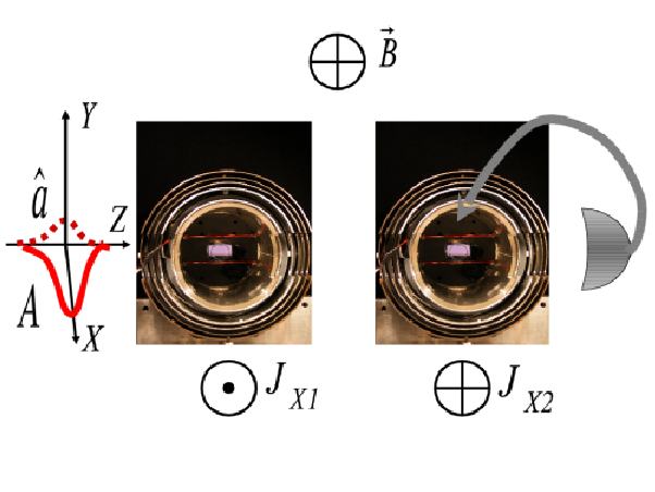
In our experiments the number of atoms is of order and we will almost always aim at having all atoms polarized along one direction which we denote as the -axis. With the -axis as quantization axis we have for all atoms to a high degree of accuracy, and the collective spin will really be a macroscopic entity. With this experimental choice, we may treat the -component of the collective spin as a classical -number, i.e. we replace the operator by the number . The transverse spin components and maintain their quantum nature. They will typically have zero or a small mean value. The quantum fluctuations are governed by the commutation relation and the Heisenberg uncertainty relation (with )
| (2) | |||
| (3) |
With atoms the quantum uncertainty of the angle of the collective spin direction is of order .
2.2 Polarization States of Light
All our experiments involve narrow-band light interacting with atomic spin states, and it turns out that the polarization states of the light form a convenient language to describe the light degrees of freedom.
Consider a pulse of light, or a collection of photons, propagating in the -direction. The polarization state is well described by the Stokes operators
| (4) |
where is the number of photons in the pulse with -polarization, and so on. The Stokes operators are dimensionless as written here, they count photons. At our convenience we will later break these up into time or spatial slices.
We make the following assumption central to the experiments described below. We assume that light consists of a strong component linearly polarized along the -direction and a much weaker component polarized in the -plane (Fig. 1). This means that we can treat the -mode operators , , and hence as a -number. Note, this is very similar to the approximation of a well polarized sample of spins in the previous section. Specifically we find (with being real) that and . We see that in our approximation the quantum properties of and are solely encoded in the -polarized part of the light.
It can be shown that the Stokes vector satisfies angular commutation relations
| (5) | |||
| (6) |
2.3 Off-Resonant Coupling
We consider the special case with a propagating beam of light coupled off-resonantly to the transitions in cesium. Then absorption effects can be neglected and all the dynamics are of dispersive nature. Furthermore, the optically excited states can be adiabatically eliminated and an effective Hamiltonian describing the light interacting with only ground state degrees of freedom is obtained (Julsgaard 2003; Hammerer et al. 2005a)11 1 (Julsgaard 2003) contains a factor of two error which has been corrected in Eq. (7)..
| (7) |
Here we have assumed a one-dimensional theory for the light which is sufficient for a beam cross section that is much larger than the squared wavelength . The small letter spin operators are dimensionless and refer to single atoms at position at time . The Stokes operators are taken to count number of photons per unit length at position and time . The integration then runs over the entire sample of length with atomic density . In the front factor is the natural FWHM line width of the optical transition and is the detuning from the to transition with red being positive.
As for the operators, is the photon flux per length, and are raising and lowering operators converting -photons into -photons or vice versa, are the usual raising and lowering operators for the spin.
The parameters , , and are for the ground state in cesium given by
| (8) |
where the limit is calculated for very large values of the detuning. The detunings MHz and MHz are given by the splitting in the excited state. Let us comment on the different terms in the Hamiltonian (7). The first term containing just gives a Stark shift to all atoms independent of the internal state but proportional to the photon density . The second term containing rotates the Stokes vector and the spin vector around the -axis, known as Faraday rotation - we look more closely into this below. The last terms proportional to are higher order couplings between the light and the atoms and since is small for a sufficiently large detuning these can normally be neglected.
All these terms conserve individually the -projection of the total angular momentum of light and atoms, e.g. the term can change a photon into a photon (changing the light angular momentum along by while the atoms receive mediated by the atomic raising operator . The total angular momentum must have its -projection invariant since the physical system is axially symmetric around the direction of light propagation (the -axis).
For us the term proportional to is useful and relevant. This term represents the QND interaction. The higher order terms proportional to create some minor problems which can be minimized with large detuning (this will be discussed further in sections B.1 and B.2). For a detailed treatment of the higher order - atomic alignment - effects we refer to (Kupriyanov et al. 2005). The zeroth order term proportional to produces an overall phase shift and can be omitted.
2.4 Propagation Equations
The Hamiltonian (7) is a very convenient starting point for many calculations and we now show the procedure to derive equations of motion. For the spin operators we need the Heisenberg evolution and for the Stokes operators the Maxwell-Bloch equations , see (Julsgaard 2003). For the latter we will neglect retardation effects, i.e. we do not calculate dynamics on the time scale of propagation across the sample. This is equivalent to setting the speed of light to infinity and hence leaving out the term. If we consider only the term proportional to and neglect the other we find
| (9) |
and
| (10) |
We observe that and are individually conserved during the interaction which is also apparent from the Hamiltonian (7) since these operators commute with the -term. The effect of the interaction is that the spin will rotate around the -axis with an amount proportional to , and the Stokes vector will rotate around the -axis proportionally with .
Below we assume that these rotations are small and that the dominant classical (mean) polarization vector of light and the orientation vector of the collective atomic spin stay oriented along the -direction after the interaction. This turns out to be a very good approximation for experimentally attainable values of the interaction strength. Under this assumption the first line of the systems (9) and (10), respectively, can be omitted. Furthermore, given the QND structure of the remaining equations, we can sum over the individual atomic spins and obtain the same equation for the collective spin variables (1). In our continuous notation we have . As for the light operators we concentrate on the in- and out-going parts only. Hence we define and . The multiplication by the speed of light turns the normalization into photons per unit time instead of per unit length. With the assumption of small rotation angles, integrating Eqs. (9) and (10) over space from to leads to the following very important equations:
| (11) | ||||
| (12) | ||||
| (13) | ||||
| (14) |
where . In and out refer to light before and after passing the atomic sample, respectively.
We note from Eqs. (11) and (14) that in the case of a large interaction strength (i.e. if dominates ) a measurement on amounts to a QND measurement of . Using off-resonant light for QND measurements of spins has also been discussed in (Kuzmich et al. 1998; Takahashi et al. 1999). Equation (13) implies that a part of the state of light is also mapped onto the atoms - we denote this as back action. This opens up the possibility of using this sort of system for quantum memory which will be the topic of sections 3.2 and 5.4.
2.5 The Rotating Frame
In the experiment a constant and homogeneous magnetic field is added in the -direction. We discuss the experimental reason for this below. For our modeling, the magnetic field adds a term to the Hamiltonian. This makes the transverse spin components precess at the Larmor frequency depending on the strength of the field. Introducing the rotating frame coordinates:
| (15) |
we can easily show that Eqs. (11)-(14) transform into:
| (16) | ||||
| (17) | ||||
| (18) | ||||
| (19) |
Thus, the atomic imprint on the light is encoded in the -sideband instead of at the carrier frequency. The primary motivation for adding the magnetic field is the fact that lasers are generally a lot more quiet at high sideband frequencies compared to the carrier. A measurement without a magnetic field will be a DC measurement and the technical noise would dominate the subtle quantum signal. Also, as the measurement time is longer than Eq. (16) enables us to access both and at the same time. We are of course not allowed to perform non-destructive measurements on these two operators simultaneously since they are non-commuting. This is also reflected by the fact that neither nor are constant in Eqs. (18) and (19). Below we shall consider two atomic samples and we will see that a QND-type interaction can be regained in this setting.
2.6 Two Oppositely Oriented Spin Samples
Inspired by the above we now assume that we have two atomic samples with oriented spins such that . We re-express the equations of motion (16)-(19) for two samples in a way which is much more convenient for the understanding of our entanglement creation and verification procedure.
For two atomic samples we write equations of motion:
| (20) | ||||
| (21) | ||||
| (22) |
The fact that the sums and have zero time derivative relies on the assumption of opposite spins of equal magnitude. The constancy of these terms together with Eq. (20) allows us to perform QND measurements on the two sums. We note that each of the sums can be accessed by considering the two operators
| (23) | ||||
| (24) |
We have used the fact that and that . Each of the operators on the left hand side can be measured simultaneously by making a -measurement and multiplying the photo-current by or followed by integration over the duration . The possibility to gain information about and enables us to generate entangled states, the topic of sections 3.1 and 5.3. At the same time we must lose information about some other physical variable. This is indeed true, the conjugate variables to these sums are and , respectively. These have the time evolution
| (25) | ||||
| (26) |
We see how noise from the input -variable is piling up in the difference components while we are allowed to learn about the sum components via measurements. The above equations clearly describe the physical ingredients for light and atoms. However, when transfer of a quantum state between two very different systems - light and atoms - is concerned, an isomorphic formulation, such as rendered by canonical variables, is desirable. In Sec. 3 we will re-write the theory in this more convenient language.
3 Quantum Information Protocols
In this chapter we introduce in detail two main protocols of this paper: deterministic generation of entanglement of two macroscopic objects and deterministic quantum state mapping from one system onto another - the so-called direct mapping protocol. The latter is then applied as the quantum memory for light protocol.
In order to simplify the description of the protocols we re-write equations of motion of the previous section in the language of canonical variables. This also allows for unified treatment of a single ensemble without- and two ensembles, with a constant magnetic field. For a single sample we define:
| (27) |
For two samples we get two sets of canonical variables by defining the atomic operators:
| (28a) | ||||
| (28b) | ||||
| (28c) | ||||
| (28d) | ||||
and the light operators:
| (29a) | ||||
| (29b) | ||||
| (29c) | ||||
| (29d) | ||||
Each pair of operators satisfy the usual commutation relation, e.g. we have . Equations (11-14) and (20-22) now translate into
| (30a) | ||||
| (30b) | ||||
| (30c) | ||||
| (30d) | ||||
where we recall refer to the definitions above and not the two samples. Note, that in the case of two samples the two sets of interacting light and atomic operators are decoupled. The parameter describing the strength of light/matter-interactions is given by . The limit to strong coupling is around . This set of equations represents the starting point for numerous applications, which in the context of this paper are implemented in the double sample setup.
3.1 Entanglement - Two Mode Squeezing Protocol
It follows from Eqs. (30a) and (30c) that a sufficiently precise measurement of of a light pulse transmitted through two atomic ensembles renders knowledge about . The measurement will project into a two-mode squeezed or Einstein-Podolsky-Rosen entangled state (Julsgaard et al. 2004a).
The necessary and sufficient condition for such an entangled state has been derived by Duan et al. 2000. Demonstration of entanglement is thus reduced to the fulfillment of this criterion. The criterion, which is introduced shortly, utilizes the vacuum state noise of a canonical variable, which for atomic ensembles reduces to the coherent spin state fluctuations. Hence, these fluctuations, which are also called projection noise, form an extremely important benchmark in experiments with atomic ensembles.
3.1.1 The Coherent Spin State
To create entangled or squeezed states one has to generate states which exhibit less fluctuations than all equivalent classical states. The boundary occurs at the coherent spin state (CSS) in which all spins are independent realizations of a single spin oriented along a specific direction. The characteristics of this state are discussed in more detail in Sec. 5.1 so for now we need only to quantify the role of the coherent spin state as a boundary between classical and purely quantum mechanical states. From the canonical atomic operators a Heisenberg uncertainty relation can be formed:
| (31) |
For the coherent spin state the two variances are both equal to one half, thus confirming that it is the classical state with the least possible noise. For a state to be squeezed, it has to have less noise in one of the quadratures. Since the Heisenberg uncertainty relation still has to be fulfilled it follows that the other quadrature has to exhibit excessive fluctuations, it is anti-squeezed. Entanglement is the non-local interconnection of two systems, such that it is impossible to write the total density matrix as a product of density matrices for each system. It has been shown that for effectively continuous variable systems such as the ones described so far in this paper the necessary and sufficient criterion for entanglement is (Duan et al. 2000)
| (32) |
3.1.2 Entanglement Generation and Verification
We now turn to the actual understanding of entanglement generation and verification. We concentrate here on generation of an entangled state conditioned on the result of a measurement. Generation of an unconditional entangled state with the help of feedback is described in the experimental section below. For generation of conditional entanglement we perform the following steps: First the atoms are prepared in the oppositely oriented coherent states corresponding to creating the vacuum states of the two modes and . Next a pulse of light called the entangling pulse is sent through the atoms and we measure the two operators and with outcomes and , respectively. These results bear information about the atomic operators and and hence we reduce variances and . To prove we have an entangled state we must confirm that the variances of and fulfill the criterion (32). That is we need to know the mean values of and with a total precision better than unity. To demonstrate that, we send a second verifying pulse through the atomic samples again measuring and with outcomes and . Now it is a matter of comparing with and with . If the results are sufficiently close the state created by the first pulse was entangled.
Let us be more quantitative. The interaction (30a) mapping the atomic operators to field operators is very useful for large and useless if . We will describe in detail the role of for all values. To this end we first describe the natural way to determine experimentally. If we repeatedly perform the first two steps of the measurement cycle, i.e. prepare coherent states of the atomic spins, send in the first measurement pulse, and record outcomes and , we may deduce the statistical properties of the measurements. Theoretically we expect from (30a)
| (33) |
The first term in the variances is the shot noise (SN) of light. This can be measured in the absence of the interaction where . The quantum nature of the shot noise level is confirmed by checking the linear scaling with photon number of the pulse. The second term arises from the projection noise (PN) of atoms. Hence, we may calibrate to be the ratio of atomic projection noise to shot noise of light. Theoretically has linear scaling with a macroscopic spin that must be confirmed in the experiment (see Sec. 5.1).
Next we describe how to deduce the statistical properties of the state created by the . Based on the measurement results and of this pulse we must predict the mean value of the second measurement outcome. If we ought to trust the first measurement completely since the initial noise of is negligible, i.e. and . On the other hand, if we know that atoms must still be in the vacuum state such that . It is natural to take in general and . We need not know a theoretical value for . The actual value can be deduced from the data. If we repeat the measurement cycle times with outcomes , , , and , the correct is found by minimizing the conditional variance
| (34) |
In order to deduce whether we fulfill the entanglement criterion (32) we compare the above to our expectation from (30a). For the verifying pulse we get
| (35) |
where refers to the incoming light of the verifying pulse which has zero mean. refers to the atoms after being entangled. We see that the practical entanglement criterion becomes
| (36) |
Simply stated, we must predict the outcomes and with a precision better than the statistical spreading of the outcomes and with the additional constraint that and are outcomes of quantum noise limited measurements.
3.1.3 Theoretical Entanglement Modeling
We described above the experimental procedure for generating and verifying the entangled states. Here we present a simple way to derive what we expect for the mean values (i.e. the -parameter) and for the variances .
We calculate directly the expected conditional variance of based on :
| (37) |
In the second step we assume that a perfect QND measurement without any decoherence is performed, i.e. . By taking the derivative with respect to we obtain the theoretical minimum
| (38) |
obtained with the -parameter
| (39) |
It is interesting that, in principle, any value of will lead to creation of entanglement. The reason for this is our prior knowledge to the entangling pulse. Here the atoms are in a coherent state which is as well defined in terms of variances as possible for separable states. We only need an “infinitesimal” extra knowledge about the spin state to go into the entangled regime.
It is also interesting to see what happens to the conjugate variables in the entangling process. This is governed by Eq. (30c). We do not perform measurements of the light operator so all we know is that both and are in the vacuum state. Hence and we preserve the minimum uncertainty relation .
3.1.4 Entanglement Model With Decoherence
Practically our spin states decohere between the light pulses and also in the presence of the light. We model this decoherence naively by attributing the entire effect to the time interval between the two pulses, i.e. we assume there is no decoherence in presence of the light but a larger decoherence between the pulses. We may then perform an analysis in complete analogy with the above with the only difference that where is a vacuum operator admixed such that corresponds to a complete decay to the vacuum state and corresponds to no decoherence. Completing the analysis we find the theoretical conditional variances
| (40) |
obtained with -parameter
| (41) |
In the limit these results agree with (38) and (39). For we have (outcomes and are useless) and the variance approaches that of the vacuum state which is a separable state.
3.1.5 Gaussian State Modeling
Following the extensive study of the evolution of Gaussian states during arbitrary interactions and measurements (Giedke and Cirac 2002; Eisert and Plenio 2003) the development of spin squeezing in a single atomic sample and entanglement in two samples were treated in detail theoretically in (Madsen and Mølmer 2004; Sherson and Mølmer 2005). Arbitrary Gaussian states of canonical modes are fully characterized by a vector, , describing the mean values and a matrix, , describing the correlations within the atomic and light systems and the cross-correlations between these. In this formalism an interaction between light and atoms is governed by: and . For the Faraday interaction, the coefficients of the matrix are easily determined from Eqs. (30). Decoherence is easily included but most importantly, there is an explicit expression for the state of the remaining modes after an arbitrary homodyne measurement on a number of the modes is performed. If the incoming pulse of light is split into a large number of segments and the interaction with atoms and subsequent measurement of each segment is treated sequentially differential equations for and can be obtained in the limit of infinitesimal segment durations. The former is a stochastic differential equation determined by the outcome of the measurement, whereas the latter is deterministic, although non-linear because of the measurement dynamics. In (Madsen and Mølmer 2004; Sherson and Mølmer 2005) such differential equations are solved giving the time resolved dynamics in the presence of e.g. atomic decoherence and light losses. In this way, e.g. analytic expressions for the optimal degree of spin squeezing and the degree of entanglement at arbitrary rotation frequencies (the verification and generalization of Eq. (38)) can be obtained easily.
3.2 Quantum Memory
For complete quantum memory we require 1) that the light state to be stored is supplied by a third party in an unknown state, 2) that this state is mapped onto an atomic state with a fidelity higher than the best classical fidelity, and finally 3) that the stored state can be retrieved from memory. As is described in Sec. 5.4 the first two criteria have been met experimentally in (Julsgaard et al. 2004a) whereas the last one still remains an unsolved experimental challenge. A recently developed experimentally feasible protocol for retrieval now exists and is discussed in Sec. 3.2.3.
3.2.1 Direct Mapping Protocol
In Eqs. (30a-30c) one of the light variables is mapped onto one of the atomic variables. This represents a natural starting point for a quantum memory protocol in which the entire light mode described by the two non-commuting variables and is faithfully stored. In the so-called ”direct mapping protocol” of (Julsgaard et al. 2004a) the mapping is completed by measuring the remaining light quadrature and feeding the result back into the atomic with a gain of :
| (42a) | ||||
| (42b) | ||||
If and the initial atomic state is assumed to be a coherent state with zero mean value the mean values of both light variables will be stored faithfully in the atoms. Although the initial atomic state has zero mean it is a quantum mechanically fluctuating state and any uncanceled atomic part will increase the noise of the final state and thus degrade the mapping performance. Although this protocol works for any state, in the following we discuss storage of coherent states of light, i.e. vacuum states which are displaced by an unknown amount in phase space. For the storage of an arbitrary coherent light state the remaining contribution limits the storage fidelity to 82%. This can be remedied by initially squeezing the atomic state, in which case 100 % fidelity can be reached in the limit of infinite squeezing.
3.2.2 Mapping With Decoherence
Just as in the case of entanglement generation the spin states decohere. Again we can model this by a beam splitter type admixture of vacuum components right after the passage of the first light pulse. We can furthermore model light damping (e.g. reflection losses) in a similar way to obtain:
| (43a) | ||||
| (43b) | ||||
We see that and are mapped with gains and respectively. The variances can be calculated easily to be:
| (44a) | ||||
| (44b) | ||||
3.2.3 Quantum Memory Retrieval
As mentioned in (Julsgaard et al. 2004a) the stored state can in principle be retrieved by inverting the roles of light and atoms in the direct mapping protocol. This would involve first an interaction between a read-out light beam with the atomic sample acting as a storage medium. According to Eq. (30a) this would map onto the light. Next has to be measured and feedback applied to the read-out beam according to the result of the measurement. However, since the atomic measurement requires a certain time during which the read-out pulse propagates at the speed of light, the feedback is only practical for pulse durations shorter than a microsecond. In the experiments of Julsgaard et al. 2004a pulses of millisecond duration () are required in order to obtain a sufficiently high interaction strength, and the inverse direct mapping protocol is thus infeasible for this experimental realization.
Several years ago a retrieval scheme, which did not involve measurements, but instead used two orthogonal passages of the read-out pulse was proposed (Kuzmich and Polzik 2003). In each passage one of the atomic quadratures is mapped onto the light pulse, and in this way retrieval fidelities of up to 82% can be achieved with coherent readout light and up to 100% with perfectly squeezed readout light. Unfortunately in order to preserve the QND nature of each of the two interactions the light has to pass entirely through the atomic medium before proceeding to the second passage. This again renders the protocol inapplicable to all setups requiring ”long” pulses.
Recently this problem was eliminated by solving the complex dynamics arising when a light beam passes through the atomic medium along two orthogonal directions simultaneously (Sherson et al. 2005b). This protocol works with arbitrary pulse durations and the fidelity of this two-pass protocol has been calculated both for a coherent input state and for a light qubit. It was also shown that if the light is reflected back after the second passage, thus completing four passages, and a time dependent interaction strength is applied perfect retrieval can be achieved without requiring squeezed initial states. In a related proposal (Fiurášek et al. 2005) retrieval is achieved by sending two different beams through the atomic samples simultaneously, each in a direction orthogonal to the other. The fidelity of retrieval for coherent states including realistic light losses is calculated and shown to exceed the classical bound.
3.2.4 Alternative Quantum Memory Proposals
In (Kuzmich and Polzik 2003) various protocols which can be implemented using the QND-Faraday interaction are described in detail, including atom-atom teleportation. Instead of reviewing these, we would like to mention some recent theoretical proposals for improving the quantum memory performance. All of these break with the simple interaction scheme either by introducing a non-QND interaction (as was also done in (Sherson et al. 2005b; Fiurášek et al. 2005)) or by exploiting the fact that the atoms involved are not simple spin-1/2 atoms and thus contain more than two magnetic sublevels.
In (Opatrny and Fiurasek 2005) it is proposed to exploit additional atomic coherences to enhance the capacity of an atomic quantum memory. Remember that during the usual QND Faraday interaction atomic coherences are coupled to the sideband of the light at the Larmor frequency. If in addition circularly polarized classical fields are present during interaction coupling between coherences and a light sideband at twice the Larmor frequency are also created. In this way an additional quantum channel is added to the quantum memory, thus enhancing its capacity. By appropriately tuning the detuning of the additional coupling field two-mode squeezer and beam splitter Hamiltonians can also be realized. With the latter, a quantum memory is realized in a single passage without a requirement of measurements or prior squeezing of atoms or light.
In (Opatrny 2005) the author proposes to create a single cell atomic memory by optically pumping the sample into an incoherent mixture of the two extreme magnetic sublevels ( and for the hyperfine level of cesium). This is done with suitable linearly polarized light. When sending a light pulse through the atomic sample it will interact with both extreme coherences simultaneously, creating the usual QND-Faraday interaction. Apart from the prospect of making the memory more compact, this proposal would also substantially decrease the reflection losses associated with the many air-glass transitions in a two-cell setup. A main problem in this approach is that in the presence of the probe light the two coherences will experience different AC-Stark shifts and thus different phase evolutions. For relevant pulse durations this effect is in fact significant. The author proposes to solve this by either decreasing the bias magnetic field or by introducing an additional AC-Stark shift by adding an light field with appropriate polarization and detuning.
An atomic memory could of course also be implemented using light-atom teleportation. This could be achieved by first sending an auxiliary pulse through the two oppositely oriented atomic samples. This would entangle the light and atomic systems via the QND-Faraday interaction. After this, the auxiliary light beam should be mixed on a 50/50 beam splitter with the quantum light signal to be teleported. Measurements of and in the two output ports respectively and subsequent feedback to the atomic system would complete the teleportation. Unfortunately the achievable fidelity is limited to 67% with the usual QND-interaction. It was therefore proposed in (Hammerer et al. 2005a) to replace the two atomic samples in the protocol just sketched by a single sample, still with a constant bias magnetic field. This changes the interaction dramatically. Both atomic quadratures are transferred to the light, albeit at the cost of additional new modes of light. The resulting multi-mode light-atom entanglement enables teleportation with up to 77% fidelity.
4 Experimental Methods

In this section we describe the typical setup for our experiments. It is centered around two glass cells filled with Cs vapor at room temperature placed in two separate magnetically insulating shields with a bias magnetic field inside. Additional coils are used to apply an rf magnetic field with the frequency equal to the Larmor frequency of the bias field. Atoms in the cells are optically pumped. The setup, therefore, is similar to that of a classical magneto-optical resonance experiment.
The typical experimental setup is shown in Fig. 2. A Verdi V8 pumped Ti:sapphire laser delivers what we call the probe field. This is used for quantum manipulation of the atomic samples and also for detecting the macroscopic spin . Diode lasers provide optical pumping fields for creating highly polarized spin states. The cw lasers are modulated by AOMs or EOMs to achieve the desired pulse shapes. Atoms are contained in vapor cells and placed in stable magnetic fields. The magnetic field homogeneity must be of order across the vapor cell volume.
4.1 Paraffin Coated Vapor Cells
In our experiments the atomic samples are contained in a paraffin coated vapor cell. The coating prevents depolarization of the spin state when atoms hit the walls. We have measured spin coherence times exceeding 40ms and spin polarizations exceeding 99% by the methods described in Sec. 4.3.1. The atomic density and thereby the macroscopic spin can be controlled by heating or cooling the vapor cell. In order to achieve a stable vapor density, temperature gradients across the cell should be avoided. Temperature control by air flow is a convenient solution. Metal heating/cooling elements causes severe problems since the atoms are disturbed by random magnetic fields created by thermal currents even if aluminum is used, see (Julsgaard 2003). Further information on paraffin coated cells can be found in (Bouchiat and Brossel 1966; Alexandrov et al. 1996; Alexandrov et al. 2002).
4.2 Detection of Polarization States

The Stokes parameters are measured with low noise photo detectors. We use high quantum efficiency photo diodes and home made amplifiers characterized by negligible electronic noise compared to the shot noise of light at optical power higher than . In Fig. 3 we depict how the -component of light is measured.
The differential photo current from the two detectors corresponds to a realization of the measurement of . By passing through a lock-in amplifier we can detect the sine and cosine components at the Larmor precession frequency . Practically, the current is multiplied by and and integrated over time for this purpose. According to (29a-d), with appropriate scaling, this exactly corresponds to measuring the and components of light. For -detection we would measure and .
4.3 Magnetic Fields
As was discussed in Sec. 2.5, external magnetic fields are added to control the dynamics of the atomic samples. The interaction of atoms with a magnetic field is governed by the Hamiltonian
| (45) |
We stress here that is the total angular momentum of the atom including the nuclear spin. For the ground state of cesium . The second term reminds us that the above linear equation is only approximately true. When the magnetic energy becomes comparable to the hyperfine splitting of the ground state the response is non-linear. We comment on this below.
Adding a constant bias magnetic field in the -direction leads to the equations of motion (15) with Larmor precession at the frequency . If we furthermore add an RF magnetic field at frequency along the -direction such that
| (46) |
with constants and we may derive for the rotating frame coordinates and of (15) that
| (47) |
with . Choosing the phase and the frequency of the RF-drive such that and we obtain:
| (48) |
These equations are valid for interaction times such that . We see that with pulses of RF-magnetic fields we are able to change the spin components and by an amount controlled by the sine and cosine components and . This has several experimental applications, which are discussed below.
4.3.1 Characterizing the Spin State with the Magneto-optical Resonance Method
Equations (20) and (47) describe the Magneto-Optical Resonance method (MORS) which we use extensively for the spin state characterization. Application of MORS to our experiments are described in detail in Julsgaard et al. 2004b. Within this method the RF frequency is scanned around and the oscillating transverse spin components are probed via oscillating polarization rotation of the optical probe. In order to quantitatively explain the MORS signal as the RF-frequency is scanned across , we need to turn back to the second order term mentioned in Eq. (45). The transverse spin components and can be expressed in terms of coherences in the following way:
| (49) |
In the absence of the second order term in (45) the energy separation between states and is the same for all and all terms have the same resonant frequency. The second order term in (45), however, makes the frequency of the coherences slightly different. It can be shown, that the frequency difference between and is where is the hyperfine splitting of the Cesium ground state. We typically have and the effect is small but detectable.
In the special case that the amplitude and frequency of the driving RF-field vary slowly compared to the spin coherence time, the off-diagonal coherences follow the diagonal populations adiabatically and we may write e.g. as:
| (50) |
where are the FWHM linewidths giving an exponential decay of each coherence. The Larmor frequency has been replaced by the individual coherence evolution frequencies . For we have to take the imaginary part. Two adjacent magnetic sublevels act as a two level system with the usual Lorentzian response to a driving RF field. Scanning the RF frequency we get eight Lorentzian peaks, the magnitudes of which will depend on the populations of the magnetic sublevels. The MORS signal is proportional to the square of the term in the square brackets in Eq. (50). An example of such a signal can be seen in Fig. 4. The application of this method is twofold. First, we gain information on the distribution of population among the different ground state magnetic sublevels. From this we infer that we are able to optically pump the atoms to such an extent that only the outermost coherence () becomes significant. Second, measuring the widths of the resonances under different experimental conditions allows us to quantify the effect of different decoherence mechanisms as discussed in Sec. 5.2.

A second implication of the second order term is that the equations of motion and describing Larmor precession are too simple and must in principle be generalized. However, this is not necessary for our case with highly polarized samples. We have almost all the population in the and states for the two samples. Then there is effectively only one non-vanishing frequency component in the sums (49). For the sample the single term is and for the sample the only term is .
4.3.2 Manipulating the Spin State
Of course, as suggested by Eq. (48), an appropriate choice of phase, strength and envelope function of the RF-field allows us to create an arbitrary mean value of either of the spins or any combination of these. This has two applications. First, it enables us to create a large classical mean value and observe the evolution of this state, thus constituting another mechanism for studying decoherence and calibrating the system as is discussed briefly at the end of Sec. B.1. Second, we can actively feed back the result of a quantum probing of the spin state, thus creating a particular desired state. This is the keystone element for creation of deterministic entanglement, discussed in Sec. 5.3.2, and for the quantum mapping experiment discussed in Sec. 5.4.
5 Experimental Results
5.1 Projection Noise Level
Since the Heisenberg uncertainty relation sets the starting point of all our calculations, one of the most important tasks in our experiments is the achievement of quantum noise limited performance. Practically, it is also one of the most difficult tasks. When we detect polarization states of light we observe noise in the signals. After the light has passed the atomic samples, there is a contribution to this noise from the light itself and from the atomic spins. The noise contribution from atoms in the minimum uncertainty state (the coherent spin state) is called the projection noise.
We discussed the ratio of the projection noise to the quantum noise of light (shot noise) already in Sec. 3.1. We found that theoretically this ratio should be
| (51) |
The ratio came from the more general interaction equations (30a-d). In the present section we discuss how to calibrate this projection noise level experimentally and how to predict the noise level from independent measurements.
5.1.1 Measuring the Macroscopic Spin
The ratio of projection noise to shot noise is proportional to the macroscopic spin . This linearity is the finger print of quantum noise and is essential to establish experimentally. To this end we need a good measure of .
We measure by detecting polarization rotation of a linearly polarized laser field propagating through the atomic samples along the -direction. To see what happens in this setting we consider Eqs. (9) and (10). These equations assume propagation along the -direction so we assume the spin to be polarized along the -direction in the following. For linearly polarized light we have and the effect on the transverse spin components , is negligible. It can also be shown easily that the and terms of the Hamiltonian (7) play no role in this calculation. We are left with the evolution of and according to (10) and after integration over the sample we find
| (52) |
where “in” refers to the polarization state before the sample at and “out” refers to the state after the sample at . The angle is given by (in radians)
| (53) |
If a linearly polarized beam of light is rotated by the angle , the Stokes vector is rotated by . Thus, in the above, is the polarization rotation caused by the spin orientation along the direction of light propagation. We note that the angle depends on the density of atoms times the length that the light traverses. We wish to re-express this in terms of the macroscopic spin size of the entire sample (remember we have the spins polarized along in this discussion). To this end we observe that where is the vapor cell volume and is the area of the vapor cell transverse to the beam direction. This will conveniently be an effective area for cells that are not exactly box like. Turning back to the usual convention of spin polarization along the -axis we then rewrite (53) as
| (54) |
5.1.2 Predicting the Projection Noise Level
Now, let us return to the predicted ratio of projection to shot noise (51). This prediction relies on Eqs. (11-14) which are derived under the assumption that all atoms in the sample are seen by the laser beam which has a cross sectional area . In experiments the laser beam does not intersect all the atoms. In App. A we show that the random motion of atoms in and out of the beam modifies the expected variance of the transverse spin components and by statistical effects from the usual to where is the mean time of an atom inside the laser beam and is the relative variance of . We furthermore present a simple model for and and show that the atomic motion will act as an effective source of decoherence between two probe pulses. We incorporate atomic motion into Eq. (51) by replacing with in the factor and multiplying the whole expression by . We then find
| (55) |
In the last step we replaced where is the optical power. We also inserted Eq. (54) to express as a function of . However, we must remember that the area in (54) refers to the transverse area for a beam propagating in the -direction while the from the relation refers to the transverse area for a beam along . Hence, the last step above is valid for a vapor cell of cubic symmetry only, but it can still be an irregularly shaped cell. In other cases the generalization is straightforward. We have reached an expression for in terms of convenient parameters from an experimental point of view. With and together with we reach our final theoretical estimate for the projection to shot noise ratio expressed in convenient units:
| (56) |
where was defined in Eq. (8).
5.1.3 Experimental Investigation


Turning to experiment, in Fig. 6 we see an example where the measured noise relative to the shot noise of light is plotted. The data are clearly linear. With MHz, ms, mW, and for the moment, we predict a linear slope of 0.140 which is somewhat higher than the measured value of 0.104. Including the from atomic motion makes the discrepancy slightly worse but given the simplicity of the theoretical model we consider the agreement satisfactory.
To test the scaling properties predicted in the atomic motion calculations, we fix the power , detuning and macroscopic spin size but vary the probe duration . The measured noise is plotted in Fig. 6 relative to the prediction (56) with . We see that as is increased we do see a lower and lower noise level which corresponds to decreasing . The solid line in the figure represents a fit where . To compare this to the simple model described in (67) we estimate our beam diameter to be 1.6cm which gives cm; moreover, cm, cm/ms (cesium at room temperature). For ms we get the prediction . This is in very good agreement with the measured data, but this agreement must be viewed as fortuitous. As mentioned before, numerical simulations of atomic motion have shown that the variance estimate (67) is almost four times too high. The high experimental value must be attributed to the additional Doppler broadening effect. We also note the relatively high uncertainty of 0.13. But all together we have a qualitative understanding of the physics and a quantitative agreement within a few tens of percent.
5.1.4 Thermal Spin Noise

Another issue concerning the projection noise level is the question of thermal spin noise. For the establishment of the correct noise level we must be in the CSS with high precision. For the CSS the spin is completely polarized along the -direction and for the ground state. As a very different example we may consider a completely unpolarized sample. We then have by symmetry . This is a factor of 10/3 higher and, even for fairly good polarization, the thermal noise may be significant. In our experiments with quantum information protocols we exceed a spin polarization of 99% which means that the thermal noise must be very small compared to the true projection noise. The degree of spin polarization has been measured independently with methods similar to those in Julsgaard et al. 2004b.
A nice illustration of the fact that we get lower noise for the CSS than in the unpolarized case is given in Fig. 7. Experimentally, we perform measurements on very poor vapor cells where the macroscopic spin life time is small. We optically pump the sample and wait for some variable delay time before probing the spin noise. For long times the spins will reach thermal equilibrium, where the noise of each atom in contributes . The fraction of atoms in is , the remaining are in the state and do not contribute because of the large detuning. Initially, all atoms are in in the CSS and they each contribute the value 2 to the noise. Hence the measured noise must be on the form
| (57) |
The predicted ratio of final to initial noise is thus . Experimentally we find the ratio which is consistent. To sum up, there is strong evidence that we really do create the CSS with the correct minimum uncertainty noise.
5.1.5 Concluding Remarks on the Projection Noise Level
Let us sum up the discussion of the projection noise level. To reach the quantum noise limited performance one should first of all observe the atomic noise grow linearly with the macroscopic spin size . An experimental example of this was shown in Fig. 6. The linearity of the noise basically arises from the fact that different atoms yield independent measurements when their spin state is detected. Technical noise sources from e.g. external electromagnetic fields couple to all atoms and the effect on the noise variance would be quadratic.
However, linearity alone is not enough. An ensemble of independent and unpolarized atoms would also show a linear increase in the spin noise when increasing the number of atoms. Since unpolarized atoms have larger noise variance than the 100% polarized atomic sample, we must know independently that the spin orientation is high. In our experiments the spin samples are polarized better than 99%.
One may argue that the small fraction of atoms that are not in the completely polarized state could, in principle, form exotic-multi particle states with a very high variance of the detected spin noise. The results discussed in Sec. 5.1.4 prove that this is not the case.
Finally, as derived in App. A the atomic motion leads to an increased ratio of atomic to shot noise. Generally a large ratio of atomic projection noise to shot noise is good for the quantum information protocols. However, we do not gain anything by the increase of the atomic noise caused by atomic motion since there will be an accompanying increase in the decoherence rate.
5.2 Decoherence
As mentioned earlier, all atoms are optically pumped into an extreme Zeeman sublevel with the -axis as quantization axis. A conventional way of categorizing sources of decoherence is according to whether they affect the magnitude of the spin along this axis or merely along transverse directions. The appropriate life times of these are called and and defined as:
| (58) |
in the absence of additional interactions. In the absence of the probe light the dominant processes are collisions with the walls and other atoms and, typically . Even though the probe detunings are quite high in our experiments (700-1200MHz) making the desired refractive Faraday interaction dominant by far, the small probability of absorption still reduces by about a factor of 2 depending on probe power and detuning. It is, however, still very large compared to typical probe durations (0.5-2 ms).
The lifetime of the transverse spin components, however, turns out to be much more critical to our experiments. As can be seen from Eq. (49) the transverse spin components are determined by coherences between magnetic sublevels in the -basis. Therefore anything that affects the lifetime of will also affect . In addition, however, the total transverse spin components are also sensitive to random phase changes in each atom. As discussed in Sec. 4.3 we can use the widths obtained in MORS signals in different experimental settings to quantify and separate the effect of different decoherence mechanisms. The FWHM obtained from such signals are related to by:
| (59) |


We can separate the mechanisms into two main categories: some are mediated by the probe light and the rest are independent of the presence of the probe. Starting with the latter, these combine to a decay rate, , and consist mainly of phase changing and spin-flip collisions with the walls and other atoms and random phase changes because of atomic motion through inhomogeneous magnetic fields. The effect of these are reduced by the paraffin coating on the inside of the glass cells, the diluteness of the atomic sample, and the application of additional dc-magnetic fields to cancel field gradients. To determine we measure the width of the coherence for different probe powers and find the residual width in the absence of light. An example of this is shown in Fig. 9. As can be seen we obtain a width of the order of 12 Hz corresponding to a lifetime of the transverse spin of . We see that this will limit but not destroy all correlations between two subsequent pulses in e.g. an entanglement experiment as described in Sec. 3.1.
Turning to the probe induced decoherence mechanism, we have already mentioned absorption and subsequent spontaneous emission in the discussion of . Adding this effect to the other decoherence mechanism, we would expect a total decoherence rate of the general form:
| (60) |
is the atomic density, is the light power, and , , and are coefficients, which can be determined experimentally. If is plotted vs. we would expect a line with constant slope and offset determined by the optical power. In Fig. 9 we show measurements of the decoherence rate vs. atomic density for different optical powers. The results clearly contradict the simple model of Eq. (60), since the slope grows with increasing power. It turns out that the experiments fit a model:
| (61) |
where the size of the expected pure power broadening term, , agrees with solutions of the Maxwell-Bloch equations for the full multi-level atomic system in the presence of Doppler broadening. The last term could represent light induced collisions, but a clear theoretical understanding of the nature of these is still missing. For the experimentally relevant densities and powers this term contributes around 30 Hz of broadening and is thus the main source of decoherence. We stress that this is a pure process since we do not observe similar features when investigating the decay of the longitudinal spin. Hence, the atoms practically decay towards the fully polarized state, i.e. the coherent spin state. This was also assumed implicitly in the inclusion of decoherence for the entanglement and quantum mapping protocols in Sec. 3, where decoherence was modeled by an admixture of a vacuum state with the same variance as the coherent spin state.
5.3 Entanglement Results
5.3.1 Conditional Entanglement


We now turn to the experimental demonstration of entanglement generation. First the boundary between the classical and the quantum fluctuations has to be established. As discussed in Sec. 5.1 this projection noise level is found by performing several measurements of as a function of the macroscopic spin size and verifying a linear increase of the atomic noise of each measurement. This linearity combined with nearly perfect orientation of the sample ensures the correct projection noise level. Once this is established we implement a probing sequence (see Fig. 2) in which the initial probing pulse is followed by a second one after a short delay. To verify entanglement we need to fulfill the criterion (36), in which case our ability to predict the outcome of the second probing of the atomic state conditioned on the result of the first measurement exceeds the classical limit.
For the experimental data we calculate the atomic part of the noise by subtracting the shot and electronics noise of a single light pulse and then normalize to the light shot noise level. In Fig. 11 the resulting atomic noise is shown for the first and second pulses (with filled and empty circles respectively). Since the measurement is of a QND-type and the variance is calculated based on 10,000 independent repetitions of the pulse sequence, the variance of the first and the second pulses should be identical. We make a quadratic + linear fit to the first pulses’ variances (dotted curve) and from this extract the linear part, which represent the coherent spin state level. The slope of this is 0.176(12), which can be compared to the theoretical values 0.187 and 0.165 obtained from Eq. (56) with and without the effect of atomic motion included. In this fit we used: T=2.0ms, P=5.0mW, and MHz. As discussed in Sec. A the results including atomic motion are very preliminary, since this is an ongoing research topic. The overall agreement with experimental results are, however, very encouraging. Note that the small quadratic component is caused by various classical noise sources.
Next we calculate the correlations between the first and the second pulse measurements as discussed in Sec. 3.1. In Fig. 11 the pulses show the conditional variance normalized to shot noise and with shot and electronics noise subtracted. The points below the straight line (36) indicate that we have in fact created an entangled state between the two atomic samples. For the highest densities the noise reduction is up to 30%. The corresponding -parameters from the minimization procedure (34) are plotted in Fig. 11 with crosses. Ideally we would expect these to follow Eq. (39) but since the atoms decohere the appropriate expression is instead Eq. (41). Fitting, we obtain , which is inserted into Eq. (40) (solid curve). Considering the fact that the solid and dash-dotted curves are obtained from a single free parameter, , the agreement between experimental results and the simple model of decoherence must be considered very satisfactory. In addition, we would like to stress the very important point that the two atomic samples, which are entangled, are in completely separate environments about 0.5 meters apart (Sherson et al. 2005a). This represents a major breakthrough towards the creation of truly distant entanglement, which combined with quantum teleportation will enable quantum communication over long distances.
5.3.2 Unconditional Entanglement
As we have just seen, the results of two probes of the spin state yield correlated results. The actual results, however, vary from shot to shot, representing random realizations of the probability distribution of the spins. That is, we create a non-local state with reduced variance but with a non-deterministic mean value. Thus, the entanglement only appears when the knowledge gained in the first pulse is applied. To create a deterministically entangled state in which no knowledge of measurement results is necessary would of course constitute a very important advance. We have realized this experimentally by simply feeding the result of the first measurement pulse back to the atoms using an RF-magnetic pulse as discussed in Sec. 4.3.2. This procedure is very closely related to the way in which unconditional spin squeezing is generated in (Geremia et al. 2004) except that there the feedback is applied continuously in time, which is more robust against errors in the feedback strength.
In the experiment we first choose a certain atomic density. Using the linear fit of Fig. 11 we find the projection noise level relative to which entanglement is estimated. Next, we vary the strength or the phase of the RF feedback pulse, and observe the variance of the second pulse fluctuations as a function of these feedback parameters. The feedback giving the lowest variance corresponds to the feedback with the optimal gain. In Fig. 11 we alternate between having feedback and not having it. As can be seen clearly, with feedback we obtain the same variance for the second pulse as we do without feedback for the conditional variance. This means that we have in fact created a state, which is deterministically entangled. That is, the state after the first probe and subsequent feedback of the measurement result has zero mean and a variance reduced by 19% compared to the projection noise level. When feedback is turned on the variance of the second pulse and the conditional variance coincide, which means that knowledge of the measurement result cannot improve the degree of entanglement beyond the entanglement proved by the second pulse measurement alone.
5.4 Quantum Memory Results
We will now present the experimental demonstration of quantum memory, which has been published in (Julsgaard et al. 2004a). The used protocol was discussed in Sec. 3.2 and, briefly, involves 1) preparation of the initial atomic state in a coherent state via optical pumping, 2) mapping of one of the light quadratures through the off-resonant Faraday interaction, Eqs. 30a-d, and 3) mapping of the second light quadrature by a direct measurement and subsequent feedback (an illustration of the timing sequence is shown in the inset of Fig. 13). For the reasons discussed in Sec. 3.2.3 we have not been able to retrieve the mapped state. Instead we have performed a destructive reconstruction of the mapped state. This is done by waiting for a time and then sending a readout light pulse through the atomic sample. Measuring the -component of the outgoing light will then give information about the stored atomic -component according to Eq. (30a). If a rotation in the atomic space is performed prior to the readout pulse we obtain information about the stored atomic -component. Repeating this 10,000 times, the statistics for the atomic variables after the storage procedure can be reconstructed. The first thing to check is that the mean value of the stored state depends linearly on the mean value of the input light state. This is shown in Fig. 13. First of all we note that the linear dependence is clear for both quadratures. This completes the proof of classical memory performance. The next thing to note is that the slope is not unity, which means that the stored state has a different mean value than the input state. The reason for this is discussed further below. For the quadrature mapped straight from the back action of the light onto the atoms we have the gain of and for the quadrature mapped via the feedback we have .


In order to verify quantum storage we also need to consider the shot-to-shot fluctuations in the stored state, which for a Gaussian state are fully characterized by the variance of the state. The experimentally reconstructed variances of the atomic quadratures, that is the variance of the readout pulse with the one unit of shot noise intrinsic to the read-out pulse subtracted, are shown in Fig. 13. Also shown is the ideal quantum limit on the variance for a perfect mapping and the classical limit for . As can be seen the variance is more or less independent of the mean value of the input light quadratures. The fidelity of the stored state for a Gaussian distribution of input states with mean photon number can be calculated given the measured gains and variances, and , according to:
| (62) |
With the experimentally measured values we get for and for . The best classical fidelity was recently derived by Hammerer et al. 2005b
| (63) |
for coherent states drawn out of a Gaussian distribution with mean photon number . This means that decreases monotonically from unity for the vacuum state to for an arbitrary coherent state. For we obtain the classical boundaries of 55.6% and 60.0% respectively. This verifies that the storage of the light state in fact constitutes a quantum mapping. The results shown were obtained for a pulse duration of 1 ms and the memory has been shown to work for up to 4 ms delay between the two probe pulses. Note that we have chosen to calculate the fidelity as the average of the squared overlap between the stored state and the ideally stored state. For non-unity gain this decreases very rapidly with coherent states having large amplitudes. However, one could argue that a storage with an arbitrary but known gain constitutes just as useful a memory as unity gain memory. If analyzed solely in terms of the added noise, our memory would therefore perform much better than the previously stated results, which can therefore be viewed as a lower bound on the memory capability.
Note also that the choice of the optimal gain which maximizes the fidelity depends on the class of available states. For classes of coherent states limited in their amplitudes discussed in this section, the experimental gains quoted above are, in fact, close to optimal ones.
5.4.1 Decoherence

In Fig. 14 we show the final atomic variances as a function of the feedback gain. These are compared to the variances expected from Eqs. (44) with independently determined decoherence values of and . We stress that this is not a fit to the data, which means that we understand the level of experimentally determined atomic noise quite well. The figure clearly shows that, because of the decoherence and light loss, if the feedback gain is increased towards unity the noise grows dramatically. With this, the fidelity quantified by Eq. (62) can be optimized with respect to the feedback gain. As can be seen from the values of and the light loss and atomic decoherence are significant. The high light loss is due to the fact that the glass cells containing the atomic vapor were not anti-reflection coated. Therefore each glass-air interface contributes about 4% loss. The main source of atomic decoherence is light assisted collisions, which change the phase of the atomic coherence without affecting the macroscopic spin size . The atoms are driven towards a coherent state, which justifies the use of the simple model of beam splitter admixture of vacuum.
6 Conclusions
We have described the progress in development of the deterministic quantum interface between light and macroscopic atomic ensembles. Theory of the interface is based on canonical variables which provide a convenient language when different physical systems, such as light and atoms, are considered. Surprisingly enough, simple dipole off-resonant interaction of light with spin polarized atomic samples with high optical density provides a powerful tool for quantum state engineering and transfer. To perform sophisticated quantum information protocols, the interaction can be combined with a quantum measurement on light and subsequent feedback to the atoms. Two central experiments of this review, entanglement of two macroscopic objects and quantum memory for light, are performed following these general steps.
Future perspectives include multipass protocols towards more efficient quantum memory including the retrieval process, as well as various types of quantum teleportation involving atomic ensembles. Another exciting future direction is demonstration of deterministic qubit state manipulation with the tool box described in this paper. It is appropriate to stress that the language of canonical variables is fully applicable not only to Gaussian states but to all single mode states, including qubit and Fock states. This language is associated with homodyne measurements in quantum optics. Addition of single photon counting to the experiments described in this article may pave the road towards more efficient and robust quantum information processing and communication.
Acknowledgements
This research has been supported by the Danish National Research Foundation and by EU grants QUICOV and COVAQIAL. B. Julsgaard is supported by the Carlsberg Foundation. We would like to thank J.I. Cirac, L.M.Duan, K. Hammerer, J. Fiurasek, A. Kozhekin, D. Kupriyanov, A. Kuzmich, and K. Mølmer for fruitful collaborations. The contributions of J. Hald and J.L. Sørensen to the early experiments are gratefully acknowledged.
References
- Alexandrov et al. (2002) Alexandrov, E. B., Balabas, M. V., Budker, D., D. English, D. F. Kimball, C.-H. L., Yashchuk, V. V. (2002). Light-induced desorption of alkali-metal atoms from paraffin coating. Phys. Rev. A 66, 042903.
- Alexandrov et al. (1996) Alexandrov, E. B., Balabas, M. V., Pasgalev, A. S., Vershovskii, A. K., Yakobson, N. N. (1996). Double-resonance atomic magnetometers: From gas discharge to laser pumping. Laser Phys. 6, 244.
- Blinov et al. (2004) Blinov, B. B., Moehring, D. L., Duan, L. M., Monroe, C. (2004). Observation of entanglement between a single trapped atom and a single photon. Nature 428, 153.
- Bouchiat and Brossel (1966) Bouchiat, M. A., Brossel, J. (1966). Relaxation of optically pumped rb atoms on paraffin-coated walls. Phys. Rev. 147, 41.
- Chaneliere et al. (2005) Chaneliere, T., Matsukevich, D. N., Jenkins, S. D., Lan, S.-Y., Kennedy, T. A. B., Kuzmich, A. (2005). Storage and retrieval of single photons transmitted between remote quantum memories. Nature 438, 833–836.
- Chou et al. (2005) Chou, C. W., de Riedmatten, H., Felinto, D., Polyakov, S. V., van Enk, S. J., Kimble, H. J. (2005). Measurement-induced entanglement for excitation stored in remote atomic ensembles. Nature 438, 828–832.
- Cirac et al. (1997) Cirac, J. I., Zoller, P., Kimble, H. J., Mabuchi, H. (1997). Quantum state transfer and entanglement distribution among distant nodes in a quantum network. Phys. Rev. Lett. 78, 3221.
- Corney and Milburn (1998) Corney, J. F., Milburn, G. J. (1998). Homodyne measurements on a bose-einstein condensate. Phys. Rev. A 58, 2399–2406.
- Duan et al. (2000) Duan, L. M., Giedke, G., Cirac, J. I., Zoller, P. (2000). Inseparability criterion for continuous variable systems. Phys. Rev. Lett. 84, 2722.
- Eisaman et al. (2005) Eisaman, M. D., Andre, A., Massou, F., Fleischhauer, M., Zibrov, A. S., Lukin, M. D. (2005). Electromagnetically induced transparency with tunable single-photon pulses. Nature 438, 837–841.
- Eisert and Plenio (2003) Eisert, J., Plenio, M. B. (2003). Introduction to the basics of entanglement theory in continuous-variable systems. Int. J. Quant. Inf. 1, 479.
- Fiurášek et al. (2005) Fiurášek, J., Sherson, J., Opatrny, T., Polzik, E. S. (2005). Single-passage read-out of atomic quantum memory, quant-ph/0510099.
- Fleischhauer and Lukin (2002) Fleischhauer, M., Lukin, M. D. (2002). Quantum memory for photons: Dark-state polaritons. Phys. Rev. A 65, 022314.
- Geremia et al. (2004) Geremia, J., Stockton, J. K., Mabuchi, H. (2004). Real-time quantum feedback control of atomic spin-squeezing. Science 304, 270.
- Giedke and Cirac (2002) Giedke, G., Cirac, J. I. (2002). Characterization of gaussian operations and distillation of gaussian states. Phys. Rev. A 66, 032316.
- Hald et al. (2005) Hald, J., Sørensen, J. L., Schori, C., Polzik, E. S. (2005). Spin squeezed atoms: A macroscopic entangled ensemble created by light. Phys. Rev. Lett. 83, 1319.
- Hammerer et al. (2005a) Hammerer, K., Polzik, E. S., Cirac, J. I. (2005a). Teleportation and spin squeezing utilizing multimode entanglement of light with atoms. Phys. Rev. A 72, 052312.
- Hammerer et al. (2005b) Hammerer, K., Wolf, M. M., Polzik, E. S., Cirac, J. I. (2005b). Quantum benchmark for storage and transmission of coherent states. Phys. Rev. Lett. 94, 150503.
- Julsgaard (2003) Julsgaard, B. (2003). Entanglement and quantum interactions with macroscopic gas samples. Ph.D. thesis, Dep. of Physics and Astronomy, University of Aarhus, Denmark, available at http://www.phys.au.dk/main/publications/PhD/.
- Julsgaard et al. (2004a) Julsgaard, B., Sherson, J., Cirac, J., Fiurášek, J., Polzik, E. (2004a). Experimental demonstration of quantum memory for light. Nature 432, 482.
- Julsgaard et al. (2004b) Julsgaard, B., Sherson, J., Sørensen, J. L., Polzik, E. S. (2004b). Characterizing the spin state of an atomic ensemble using the magneto-optical resonance method. J. Opt. B: Quantum Semiclass. Opt. 6, 5.
- Kozhekin et al. (2000) Kozhekin, A. E., Mølmer, K., Polzik, E. S. (2000). Quantum memory for light. Phys. Rev. A 62, 033809.
- Kuhn et al. (2002) Kuhn, A., Hennrich, M., Rempe, G. (2002). Deterministic single-photon source for distributed quantum networking. Phys. Rev. Lett. 89, 067901.
- Kupriyanov et al. (2005) Kupriyanov, D., Mishina, O., Sokolov, I., Julsgaard, B., Polzik, E. (2005). Multimode entanglement of light and atomic ensembles via off-resonant coherent forward scattering. Phys. Rev. A 71, 032348.
- Kuzmich et al. (1998) Kuzmich, A., Bigelow, N. P., Mandel, L. (1998). Atomic quantum non-demolition measurements and squeezing. Europhys. Lett. 42, 481.
- Kuzmich et al. (2003) Kuzmich, A., Bowen, W. P., Boozer, A. D., Boca, A., Chou, C. W., Duan, L. M., Kimble, H. J. (2003). Generation of nonclassical photon pairs for scalable quantum communication with atomic ensembles. Nature 423, 731.
- Kuzmich and Kennedy (2004) Kuzmich, A., Kennedy, T. A. B. (2004). Nonsymmetric entanglement of atomic ensembles. Phys. Rev. Lett. 92, 030407.
- Kuzmich et al. (2000) Kuzmich, A., Mandel, L., Bigelow, N. P. (2000). Generation of spin squeezing via continuous quantum nondemolition measurement. Phys. Rev. Lett. 85, 1594.
- Kuzmich et al. (1997) Kuzmich, A., Mølmer, K., Polzik, E. S. (1997). Spin squeezing in an ensemble of atoms illuminated with squeezed light. Phys. Rev. Lett. 79, 4782.
- Kuzmich and Polzik (2003) Kuzmich, A., Polzik, E. S. (2003). Quantum Infomation with Continuous Variables. Kluwer, Dordrecht, pp. 231–265, eds. S. L. Braunstein and A. K. Pati.
- Madsen and Mølmer (2004) Madsen, L. B., Mølmer, K. (2004). Spin squeezing and precision probing with light and samples of atoms in the gaussian description. Phys. Rev. A 70, 052324.
- Madsen and Mølmer (2004) Madsen, L. B., Mølmer, K. (2004). Spin squeezing and precision probing with light and samples of atoms in the gaussan description. Phys. Rev. A 70, 052324.
- McKeever et al. (2004) McKeever, J., Boca, A., Boozer, A. D., Miller, R., Buck, J. R., Kuzmich, A., Kimble, H. J. (2004). Deterministic generation of single photons from one atom trapped in a cavity. Science 303, 1992.
- Opatrny (2005) Opatrny, T. (2005). Single-cell atomic quantum memory for light, quant-ph/0509094.
- Opatrny and Fiurasek (2005) Opatrny, T., Fiurasek, J. (2005). Enhancing the capacity and performance of collective atomic quantum memory. Phys. Rev. Lett. 95, 053602.
- Polzik (2004) Polzik, E. S. (2004). Quantum information: Flight of the qubit. Nature 428, 129.
- Raimond et al. (2001) Raimond, J. M., Brune, M., Haroche, S. (2001). Manipulating quantum entanglement with atoms and photons in a cavity. Rev. Mod. Phys. 73, 565.
- Sanders and Milburn (1989) Sanders, B. C., Milburn, G. J. (1989). Quantum nondemolition measurement of quantum beats and the enforcement of complementarity. Phys. Rev. A 40, 7087–7092.
- Sherson et al. (2005a) Sherson, J., Julsgaard, B., Polzik, E. S. (2005a). Distant entanglement of macroscopic samples. In: W. M. Akulin, A. Sarfati, G. K., Pellegrin, S. (Eds.), Decoherence, Entanglement and Information Protection in Complex Quantum Systems. NATO Science Series II. Springer, Dordrecht, pp. 353–372.
- Sherson and Mølmer (2005) Sherson, J., Mølmer, K. (2005). Entanglement of large atomic samples: a gaussian state analysis. Phys. Rev. A 71, 033813.
- Sherson et al. (2005b) Sherson, J., Sørensen, A. S., Fiurášek, J., Mølmer, K., Polzik, E. (2005b). Light qubit storage and retrieval using macroscopic atomic ensembles, quant-ph/0505170.
- Takahashi et al. (1999) Takahashi, Y., Honda, K., Tanaka, N., Toyoda, K., Ishikawa, K., Yabuzaki, T. (1999). Quantum nondemolition measurement of spin via the paramagnetic faraday rotation. Phys. Rev. A 60, 4974.
- Thomsen et al. (2002) Thomsen, L. K., Mancini, S., Wiseman, H. M. (2002). Continuous quantum non-demolition feedback and unconditional atomic spin squeezing. Journal of Phys. B 35, 4937–4952.
- van der Wal et al. (2003) van der Wal, C. H., Eisaman, M. D., Andre, A., Walsworth, R. L., Phillips, D. F., Zibrov, A. S., Lukin, M. D. (2003). Atomic memory for correlated photon states. Science 301, 196.
- Volz et al. (2005) Volz, K., Weber, M., Schlenk, D., Rosenfeld, W., Vrana, J., Saucke, K., Kurtsiefer, C., Weinfurter, H. (2005). Atom-photon entanglement, quant-ph/0511183, to appear in Phys. Rev. Lett.
- Wiseman (1998) Wiseman, H. M. (1998). In-loop squeezing is like real squeezing to an in-loop atom. Phys. Rev. Lett. 81, 3840–3843.
- Zoller et al. (2005) Zoller, P., Beth, T., Binosi, D., Blatt, R., Briegel, H., Bruss, D., Calarco, T., Cirac, J., Deutsch, D., Eisert, J., Ekert, A., Fabre, C., Gisin, N., Grangier, P., Grassl, M., Haroche, S., Imamoglu, A., Karlson, A., Kempe, J., Kouwenhoven, L., Kröll, S., Leuchs, G., Lewenstein, M., Loss, D., Lütkenhaus, N., Massar, S., Mooij, J., Plenio, M., Polzik, E., Popescu, S., Rempe, G., Sergienko, A., adn J. Twamley, D. S., Wendin, G., Werner, R., Winter, A., Wrachtrup, J., Zeilinger, A. (2005). Quantum information processing and communication: Strategic report on current status, visions and goals for research in europe. European Physical Journal D 36 (2), 203–228.
Appendix A Effect of Atomic Motion
Since in our experiments the atoms are at room temperature and, for experimental reasons, the light beam does not cover the entire cross section of the atomic sample, the atoms move across the beam several times () during the time of a pulse. This averaging effect insures that all atoms spend roughly the same amount of time inside the beam but, as we shall see, it still has important implications for the noise properties. In brief, the atomic motion modifies the projection noise level and acts as an additional source of decoherence since two subsequent probe pulses interact with the atoms differently. The results are related to the work of Kuzmich and Kennedy 2004.
A.1 Modeling Atomic Motion
To be more quantitative, we introduce new pseudo-angular momentum operators , where is the fraction of time the ’th atom spends interacting with the laser beam and . These have the commutator:
| (64) |
This leads to the Heisenberg uncertainty relation (for a highly polarized sample with )
| (65) |
where we have introduced the mean and variance of . With this definition, is the relative standard deviation of . Since, for the coherent spin state,
| (66) |
this highly polarized state corresponds to a minimum uncertainty state. The measured noise is then limited by the Heisenberg uncertainty principle and we confidently call this projection noise. To maintain the correct commutation relation we experimentally normalize the atomic operators to the measured projection noise, i.e. instead of defining we effectively have .
The average fraction of time each atom spends inside the beam is clearly . Let us now discuss the scaling of with simple physical parameters. The fact that the variance may be non-zero arises from the finite time available for the averaging process carried out by the atomic motion. A typical traversing time across the vapor cell is where is the cell dimension and is e.g. the one-dimensional rms speed of the atoms. We may think of this atomic motion as independent journeys across the vapor cell volume, where . We then model the motion through the beam with mean occupancy by assuming in each walk across the cell volume that either (1) the atom spends all the time inside the beam, which should happen with probability , or (2) the atom spends all the time outside the beam which should happen with probability .
We then count the number of times that an atom was inside the beam out of the possible journeys. In this simple model is a stochastic variable which is binomially distributed with mean and variance . We are interested in the fraction of time () spent inside the beam. It follows and . Hence the simple model leads to
| (67) |
Note the characteristic scaling with and with the area not covered by the light beam (when is close to its maximum value ). We note that due to the simplicity of the above model the absolute numbers should only hold as an order of magnitude estimate. Numerical simulations performed for a cubic cell have shown that the relative variance is roughly four times smaller than the estimate above. Also, due to the Doppler broadening, the effective detuning differs from atom to atom and causes an increase in .
A.2 Atomic Motion as a Source of Decoherence
To see how atomic motion acts as an effective source of decoherence, imagine that we perform some manipulations of atoms using one laser pulse and subsequently probe these manipulations with another laser pulse. Since atoms move during interactions the probed quantum operator changes in time. Comparing the operator at the 1st and 2nd times we get
| (68) |
We assumed and to be uncorrelated, which is reasonable since a collision with the cell wall randomizes the velocity of the atoms. Also, we took . This corresponds to having no decoherence at all apart from the effect of atomic motion which is the only effect studied in this calculation. To interpret the above calculations we consider a standard decoherence calculation. Consider a true spin operator subject to decoherence parametrized by the number such that
| (69) |
Then the operator changes by an amount characterized by the variance
| (70) |
which is exactly the same as in (68). We are led to the conclusion that atomic motion inevitably gives rise to an effective decoherence. We thus see that, whereas the increased coherent spin state noise with increased might seem to suggest that non-classical states are more easily created (by producing states with noise lower than the CSS), this is compensated for by an increased decoherence of the state. Therefore, higher does not lead to higher fidelity protocols.
Appendix B Technical Details
B.1 Light Polarization and Stark Shifts
Let us calculate the Stark effect from the probe laser on the magnetic sublevels . We let the light be strong and linearly polarized along the vector
| (71) |
i.e. is the angle between the macroscopic spin direction (the -axis) and the probe polarization direction. Light is propagating in the -direction. The Stark effect on magnetic sub-levels is much weaker than the splitting caused by the constant bias magnetic field and can be calculated in non-degenerate perturbation theory from the interaction Hamiltonian (7). The term is common to all levels, the term is zero on average since , and we are left with the higher order components proportional to .
With being the creation operator along the strong direction we have and (neglecting the orthogonal direction to which will be in the vacuum state for linear polarization). With we derive from (4) that
| (72) |
where is the photon flux and Stokes operators are normalized to photons per second. In order to calculate the higher order terms of the interaction Hamiltonian for a single atom we leave out the integral in (7) and renormalize light operators (by absorbing the speed of light ) to photons per second and find
| (73) |
We also replaced by . We need to calculate the expectation value of this Hamiltonian for the different energy eigenstates quantized along the -direction. We have
| (74) |
The first of these is obvious since is quantized along the -axis. We have by symmetry and the value is found from the fact that . Also, by symmetry we have in an eigenstate of that which leads to the final line. Calculating the expectation value of (73) we get
| (75) |
What is important for us is the shift of a magnetic resonance line which then becomes
| (76) |
This Stark shift is problematic for several protocols, especially the setup with two oppositely oriented samples. Note, that for atoms polarized in the state the relevant transition has a Stark shift proportional to . An oppositely oriented sample with has for the transition a Stark shift proportional to . Hence, these two transition frequencies cannot be overlapped both in the presence and absence of light (see Fig. 15 for an illustration).

One remedy for this is to choose the light to be linearly polarized at an angle corresponding to , and the Stark term disappears. As we shall see in Sec. B.2 this gives rise to other problems.
Another remedy is to add an extra bias magnetic field along the -direction when the laser light is on. In this way the frequency of the desired transitions can be kept stable. This is the approach we have taken and it works well. One should note though, that with our laser pulse timing in the vicinity of one millisecond, it is not completely trivial to make a magnetic pulse following the laser intensity since eddy currents in metallic parts and induced electric fields in other current loops for magnetic fields should be taken into account. A convenient diagnostic method is to apply a classical shift to the spin states along the lines of Eq. (48) prior to the application of two laser pulses. An detection of the light will show in real time the mean value of the spin state components and . These should be constant through each laser pulse and conserved in the dark time in between (apart from a possible decay) if all frequencies are well adjusted.
B.2 Influence of Laser Noise
In this section we make a brief comment on laser noise entering the atomic samples. This is by no means a complete analysis but it describes some important issues in connection with the choice of laser polarization. We start out with the interaction Hamiltonian (7) and also assume that the atoms are polarized along the -axis and placed in a bias magnetic field, leading to the magnetic Hamiltonian . This leads to the following equations of motion for the transverse spin components and :
| (77) | ||||
| (78) |
The Larmor precession terms take all interesting dynamics to the frequency component around . Let us see which terms above couple -components of light into the spin state. First, the term is our favorite interaction term (13) used in all quantum information protocols. It consists of an atomic operator which is constant equal to for all practical purposes. This is multiplied by , whose -components drive .
In Eq. (78) the final term is proportional to . Practically, this is also constant equal to . It is then multiplied by , whose -components drive . This is an unwanted effect. The ratio of the unwanted to wanted noise is found by squaring these contributions. We get
| (79) |
For our typical values of detuning we have and the above ratio becomes for . If our laser beam is polarized along the - or -axis with a clean linear polarization, the noise of and at frequency can be shot noise limited, i.e. by quantum noise (amplitude noise of the laser does drive into and in the case of clean linear polarization). In this case the unwanted noise only contributes of the total noise pile up. But if we choose arbitrary polarization directions in the -plane, the -component will have non-zero mean value, and the fluctuations at will essentially be the amplitude noise of the laser at . In this case, to keep the last term of Eq. (78) from accumulating extra noise, one requires the laser intensity to be shot noise limited at (which is a more difficult condition to meet than clean linear polarization). We thus have one motivation for choosing the laser to be polarized along the - or -direction and not in between. We typically do this in our experiments and for this reason we have to compensate the Stark splitting discussed in Sec. B.1. For a further discussion of the different higher order terms in the interaction, see (Julsgaard 2003). A more thorough discussion of quantum noise with the higher order terms included is given by Kupriyanov et al. 2005.