跳到论文正文
W Papers独立论文阅读器 arXiv:quant-ph/0512069 论文正文 计算阅读时间 · 0%
引用这篇论文根据当前论文元数据生成,正式投稿前建议核对。


License: Assumed arXiv.org perpetual non-exclusive license
arXiv:quant-ph/0512069v2 [quant-ph] 22 Feb 2006

Entanglement evaluation of non-Gaussian states generated by photon subtraction from squeezed states

Akira Kitagawa Email: kitagawa@nict.go.jp Affiliation: National Institute of Information and Communications Technology (NICT) 4-2-1 Nukui-Kita, Koganei, Tokyo 184-8795 Japan Affiliation: Core Research for Evolutional Science and Technology (CREST), Japan Science and Technology Agency
1-9-9 Yaesu, Chuoh, Tokyo 103-0028 Japan
   Masahiro Takeoka Affiliation: National Institute of Information and Communications Technology (NICT) 4-2-1 Nukui-Kita, Koganei, Tokyo 184-8795 Japan Affiliation: Core Research for Evolutional Science and Technology (CREST), Japan Science and Technology Agency
1-9-9 Yaesu, Chuoh, Tokyo 103-0028 Japan
   Masahide Sasaki Affiliation: National Institute of Information and Communications Technology (NICT) 4-2-1 Nukui-Kita, Koganei, Tokyo 184-8795 Japan Affiliation: Core Research for Evolutional Science and Technology (CREST), Japan Science and Technology Agency
1-9-9 Yaesu, Chuoh, Tokyo 103-0028 Japan
   Anthony Chefles Affiliation: School of Mathematical Sciences, University College Dublin, Dublin 4, Ireland
August 11, 2026
Abstract

We consider the problem of evaluating the entanglement of non-Gaussian mixed states generated by photon subtraction from entangled squeezed states. The entanglement measures we use are the negativity and the logarithmic negativity. These measures possess the unusual property of being computable with linear algebra packages even for high-dimensional quantum systems. We numerically evaluate these measures for the non-Gaussian mixed states which are generated by photon subtraction with on/off photon detectors. The results are compared with the behavior of certain operational measures, namely the teleportation fidelity and the mutual information in the dense coding scheme. It is found that all of these results are mutually consistent, in the sense that whenever the enhancement is seen in terms of the operational measures, the negativity and the logarithmic negativity are also enhanced.

pacs
03.67.Mn, 03.67.Hk, 42.50.Dv

I Introduction

Continuous variable (CV) quantum optical systems are well-established tools for both theoretical and experimental investigations of quantum information processing (QIP) Nielsen; Braunstein03. The essential resource, entanglement, can be realized with a Gaussian two-mode squeezed vacuum state. This state is relatively easy to work with theoretically and is also commonly produced in the laboratory. It has been successfully applied to implement various important protocols, such as quantum teleportation Braunstein98; Furusawa98; Zhang03; Bowen03, quantum dense coding Ban99; Li02; Mizuno05 and entanglement swapping Jia04; Takei05. These successes are based on well-developed techniques of optical Gaussian operations. These consist of beam splitting, phase shifting, squeezing, displacement and homodyne detection.

However, recent theoretical investigations have shown some limits on such operations. A prime example is the no-go theorem relating to the distillation of entanglement shared by distant parties using only Gaussian local operations and classical communication (LOCC) Eisert02; Fiurasek02; Giedke02. To go beyond this limit, one should use higher order nonlinear processes, such as the cubic-phase gate Gottesman01 or Kerr nonlinearity Nemoto04. It is, however, difficult to implement these nonlinear processes with presently available materials, which do not have sufficiently high nonlinearity and suffer from losses. A more practical alternative method has been developed, which uses nonlinear processes induced by photon counting on tapped-off beams from squeezed states Opatrny00; Cochrane02; Browne03. When ideal photon number resolving detectors are used, the input Gaussian state can be transformed into a non-Gaussian pure state with higher entanglement. In practice, however, such detectors are not yet suitable for practical use. The most reliable type of photodetector available at present is the on/off type photon detector based on avalanche photodiodes. This device can only distinguish the vacuum (‘off’) state from non-vacuum (‘on’) states. The latter events result in a non-Gaussian mixed state. Evaluating the entanglement of such a state is far from trivial.

Previously, the effect of entanglement has been theoretically analysed based on the figures of merit of concrete protocols, such as the fidelity of teleportation Olivares03, the degree of violation of Bell-type inequalities Nha04; Garcia-Patron04; Olivares04 and the mutual information of dense coding Kitagawa05. In fact, it was shown that the performance of every protocol was improved, implying that the entanglement of the non-Gaussian mixed state must be enhanced. However, these indirect evaluations were dependent upon some external parameters, which depend upon specific operations differing from protocol to another, such as the type of input state for the teleportation fidelity, the choice of the measurement basis for the Bell-type inequality violation, and the signal power of modulation for the dense coding.

Quantifying the entanglement of the photon-subtracted squeezed state, in a way which is independent of particular external parameters, is our main concern in this paper. To our knowledge, this problem has not been previously addressed. For a state ρ^\hat{\rho}, an entanglement measure E⁡(ρ^)E(\hat{\rho}) should satisfy the following criteria Vidal00: (i) EE is the non-negative functional, (ii) EE vanishes if the state ρ^\hat{\rho} is separable and (iii) EE should not increase on average under LOCC. In general, a quantity satisfying these criteria is known as an entanglement monotone. Many such quantities have been proposed, such as the entanglement of formation Bennett96-2; Wootters98, the entanglement cost Hayden01, the distillable entanglement Bennett96-2, and the relative entropy of entanglement Vedral98. It is, however, not easy to calculate these measures for generic mixed states. Recently, however, two entanglement measures which are much more amenable to evaluation have been proposed. These are the negativity and the logarithmic negativity Vidal02. These measures are based on the Peres criterion Peres96. That is, they are defined in terms of the eigenvalues of the partially-transposed density operator. The most distinctive feature of these entanglement measures is that they are easily computable numerically with linear algebra packages. Furthermore, the logarithmic negativity is an additive functional, and it is an upper bound on the distillable entanglement EDE_{\rm D} Vidal02.

In addition to being an entanglement monotone, it was believed that an entanglement measure EE should also be (downward) convex, i.e. it should be non-increasing on average under the loss of classical information by mixing. Convexity is necessary for an entanglement measure to be bounded from above by the entanglement of formation EFE_{\rm F} Horodecki00, although the logarithm function is concave (upward convex). Recently, however, it has been shown by Plenio et al Plenio05; Plenio05-2 that convexity is not directly related to the physical process of discarding quantum information, i.e. discarding subsystems such as local ancillas during LOCC operations and that the logarithmic negativity is indeed a full entanglement monotone Plenio05-2. In view of these considerations, it is interesting to evaluate the entanglement of photon-subtracted mixed state in terms of the (logarithmic) negativities, and to compare them the figures of merit associated with the aforementioned protocols. Of particular interest to us is how the entanglement, and these figures of merit, are enhanced by the photon-subtraction procedure.

This paper is organized as follows. In Sec. II, we briefly summarize the measurement-induced non-Gaussian operation on the two-mode squeezed vacuum state and its mathematical description. In Sec. III, the negativity and the logarithmic negativity are briefly reviewed, and their monotonicity is discussed. In Sec. IV, our numerical methods for calculating the negativities of the photon-subtracted mixed state are presented. In Sec. V, we review the previous analyses of the entanglement of such states using protocol-specific figures of merit. We compare these results with those relating to the negativity/logarithmic negativity. The final section VI is devoted to discussion and conclusion.

II Measurement-induced non-Gaussian operation

The schematic of the measurement-induced non-Gaussian operation on the two-mode squeezed state is shown in Fig. 1.

Refer to caption
Figure 1: Measurement-induced non-Gaussian operation on the two-mode squeezed vacuum state. BS, PS are beam splitter, photon detector, respectively.

The primary sources are two identical, single-mode squeezed vacuum states,

|r⟩k=S^k​(r)​|0⟩k,|r\rangle_{k}=\hat{S}_{k}(r)|0\rangle_{k}, (1)

where S^k​(r)\hat{S}_{k}(r) is the squeezing operator at path kk,

S^k​(r)=exp⁡[−r2​(a^k†2−a^k2)],\hat{S}_{k}(r)=\exp\left[-\frac{r}{2}(\hat{a}_{k}^{\dagger 2}-\hat{a}_{k}^{2})\right], (2)

and rr is the squeezing parameter. These are combined via a balanced beam splitter to generate the two-mode squeezed vacuum state,

|r(2)⟩AB\displaystyle|r^{(2)}\rangle_{\rm AB} =\displaystyle= V^AB​(π4)​|r⟩A​|−r⟩B\displaystyle\hat{V}_{\rm AB}\left(\frac{\pi}{4}\right)|r\rangle_{\rm A}|-r\rangle_{\rm B} (3)
=\displaystyle= S^AB​(−r)​|0⟩AB\displaystyle\hat{S}_{\rm AB}(-r)|0\rangle_{\rm AB}
=\displaystyle= ∑n=0∞αn​|n⟩A​|n⟩B,\displaystyle\sum_{n=0}^{\infty}\alpha_{n}|n\rangle_{\rm A}|n\rangle_{\rm B},

where

V^k​l​(θ)=exp⁡[θ⁡(a^k†​a^l−a^k​a^l†)]\hat{V}_{kl}(\theta)=\exp\left[\theta(\hat{a}_{k}^{\dagger}\hat{a}_{l}-\hat{a}_{k}\hat{a}_{l}^{\dagger})\right] (4)

is the beam splitter operator, and the parameter θ\theta is related to the transmittance TT as

tan⁡θ=1−TT,\tan\theta=\sqrt{\frac{1-T}{T}}, (5)

and θ=π/4\theta=\pi/4 corresponds to the balanced beam splitter. The operator S^k​l(2)​(r)\hat{S}^{(2)}_{kl}(r) is the two-mode squeezing operator,

S^k​l(2)​(r)=exp⁡[−r⁡(a^k†​a^l†−a^k​a^l)].\hat{S}^{(2)}_{kl}(r)=\exp\left[-r(\hat{a}_{k}^{\dagger}\hat{a}_{l}^{\dagger}-\hat{a}_{k}\hat{a}_{l})\right]. (6)

Introducing λ=tanh⁡r\lambda=\tanh r, the Schmidt coefficients are given by

αn=1−λ2​λn.\alpha_{n}=\sqrt{1-\lambda^{2}}\lambda^{n}. (7)

The beam at path C (D) is then tapped off from path A (B) by a beam splitter of transmittance TT. The resulting four-mode state just after the second beam splitters is

|ψ⟩ABCD\displaystyle|\psi\rangle_{\rm ABCD} =\displaystyle= V^BD​(θ)​V^AC​(θ)​|r(2)⟩AB​|0⟩CD\displaystyle\hat{V}_{\rm BD}(\theta)\hat{V}_{\rm AC}(\theta)|r^{(2)}\rangle_{\rm AB}|0\rangle_{\rm CD}
=\displaystyle= ∑nαn​∑i,j=0nξn​i​ξn​j​|n−i⟩A​|n−j⟩B​|i⟩C​|j⟩D,\displaystyle\sum_{n}\alpha_{n}\sum_{i,j=0}^{n}\xi_{ni}\xi_{nj}|n-i\rangle_{\rm A}|n-j\rangle_{\rm B}|i\rangle_{\rm C}|j\rangle_{\rm D},

where

ξn​k=(−1)k​(nk)​(T)n−k​(R)k,\xi_{nk}=(-1)^{k}\sqrt{\binom{n}{k}}\left(\sqrt{T}\right)^{n-k}\left(\sqrt{R}\right)^{k}, (9)

and (nk)\binom{n}{k} is the binomial coefficient and R=1−TR=1-T is the reflectance.

II.1 Photon number resolving detector case

When kk photons are detected in the beam at path C and ll are detected in path D by ideal photon number resolving detectors, the conditional state is given by

|ψNG(k​l)⟩AB\displaystyle|\psi_{\rm NG}^{(kl)}\rangle_{\rm AB} ∝\displaystyle\propto ⟨l|⟨k|ψ⟩ABCDCD\displaystyle{{}_{\rm D}\langle}l|{{}_{\rm C}\langle}k|\psi\rangle_{\rm ABCD}
=\displaystyle= ∑n=max⁡{k,l}∞αn​ξn​k​ξn​l​|n−k⟩A​|n−l⟩B,\displaystyle\sum_{n=\max\{k,l\}}^{\infty}\alpha_{n}\xi_{nk}\xi_{nl}|n-k\rangle_{\rm A}|n-l\rangle_{\rm B},

where |ψNG⟩AB|\psi_{\rm NG}\rangle_{\rm AB} is still a pure state. In the case of k=l=1k=l=1,

|ψNG(1)⟩AB\displaystyle|\psi_{\rm NG}^{(1)}\rangle_{\rm AB} =\displaystyle= 1Pdet(1)​∑n=0∞αn+1​ξ(n+1),12​|n⟩A​|n⟩B\displaystyle\frac{1}{\sqrt{P_{\rm det}^{(1)}}}\sum_{n=0}^{\infty}\alpha_{n+1}\xi_{(n+1),1}^{2}|n\rangle_{\rm A}|n\rangle_{\rm B} (11)
=\displaystyle= ∑n=0∞cn(1)​|n⟩A​|n⟩B,\displaystyle\sum_{n=0}^{\infty}c_{n}^{(1)}|n\rangle_{\rm A}|n\rangle_{\rm B},

where

Pdet(1)\displaystyle P_{\rm det}^{(1)} =\displaystyle= ∑n=0∞|αn+1|2​|ξ(n+1),12|2\displaystyle\sum_{n=0}^{\infty}|\alpha_{n+1}|^{2}|\xi_{(n+1),1}^{2}|^{2} (12)
=\displaystyle= (1−λ2)​λ2​T2​(1+λ2​T2)(1−λ2​T2)3​(RT)2\displaystyle\frac{(1-\lambda^{2})\lambda^{2}T^{2}(1+\lambda^{2}T^{2})}{(1-\lambda^{2}T^{2})^{3}}\left(\frac{R}{T}\right)^{2}

is the probability of detecting one photon in each arm. The state (11) is not Gaussian any more.

II.2 On/off type detector case

An ideal on/off type detector is described by a positive operator-valued measure (POVM) with elements

{Π^(off)=|0⟩​⟨0|,Π^(on)=|1⟩​⟨1|+|2⟩​⟨2|+⋯=1^−|0⟩​⟨0|.\left\{\begin{array}[]{lcl}\hat{\Pi}^{(\rm off)}&=&|0\rangle\langle 0|,\\ \hat{\Pi}^{(\rm on)}&=&|1\rangle\langle 1|+|2\rangle\langle 2|+\cdots=\hat{1}-|0\rangle\langle 0|.\end{array}\right. (13)

The two-mode squeezed state is transformed into a mixed non-Gaussian state

ρ^NG\displaystyle\hat{\rho}_{\rm NG} =\displaystyle= TrCD​[|ψ⟩(ABCD)​⟨ψ|⊗(Π^C(on)⊗Π^D(on))]𝒫det\displaystyle\frac{{\rm Tr}_{\rm CD}\left[|\psi\rangle_{\rm(ABCD)}\langle\psi|\otimes\left(\hat{\Pi}^{\rm(on)}_{\rm C}\otimes\hat{\Pi}^{\rm(on)}_{\rm D}\right)\right]}{\mathcal{P}_{\rm det}} (14)
=\displaystyle= 1𝒫det​∑i,j=1∞|Φi​j⟩(AB)​⟨Φi​j|,\displaystyle\frac{1}{\mathcal{P}_{\rm det}}\sum_{i,j=1}^{\infty}|\Phi_{ij}\rangle_{\rm(AB)}\langle\Phi_{ij}|,

where

|Φi​j⟩AB=∑n=max⁡{i,j}αn​ξn​i​ξn​j​|n−i⟩A​|n−j⟩B,|\Phi_{ij}\rangle_{\rm AB}=\sum_{n=\max\{i,j\}}\alpha_{n}\xi_{ni}\xi_{nj}|n-i\rangle_{\rm A}|n-j\rangle_{\rm B}, (15)

and 𝒫det\mathcal{P}_{\rm det} is the probability of detecting at least one photon in each of the paths C and D,

𝒫det\displaystyle\mathcal{P}_{\rm det} =\displaystyle= TrABCD​[|ψ⟩(ABCD)​⟨ψ|⊗(Π^C(on)⊗Π^D(on))]\displaystyle{\rm Tr}_{\rm ABCD}\left[|\psi\rangle_{\rm(ABCD)}\langle\psi|\otimes\left(\hat{\Pi}^{\rm(on)}_{\rm C}\otimes\hat{\Pi}^{\rm(on)}_{\rm D}\right)\right] (16)
=\displaystyle= λ2​(1−T)2​(1+λ2​T)(1−λ2​T)​(1−λ2​T2).\displaystyle\frac{\lambda^{2}(1-T)^{2}(1+\lambda^{2}T)}{(1-\lambda^{2}T)(1-\lambda^{2}T^{2})}.

The mean photon number of the state ρ^NG\hat{\rho}_{\rm NG} is expressed as

N¯NG\displaystyle\bar{N}_{\rm NG} =\displaystyle= TrAB​[ρ^NG⊗(N^A+N^B)]\displaystyle\textrm{Tr}_{\rm AB}\left[\hat{\rho}_{\rm NG}\otimes\left(\hat{N}_{\rm A}+\hat{N}_{\rm B}\right)\right] (17)
=\displaystyle= 2​(1−λ2)𝒫det[λ2​T(1−λ2)2−λ2​T(1−λ2​T)2\displaystyle\frac{2(1-\lambda^{2})}{\mathcal{P}_{\rm det}}\Bigg[\frac{\lambda^{2}T}{(1-\lambda^{2})^{2}}-\frac{\lambda^{2}T}{(1-\lambda^{2}T)^{2}}
−λ2​T2(1−λ2​T)2+λ2​T2(1−λ2​T2)2],\displaystyle\hskip 28.45274pt-\frac{\lambda^{2}T^{2}}{(1-\lambda^{2}T)^{2}}+\frac{\lambda^{2}T^{2}}{(1-\lambda^{2}T^{2})^{2}}\Bigg],

In Fig. 2, the mean photon number N¯NG\bar{N}_{\rm NG} is shown as a function of λ\lambda, with that of the two-mode squeezed vacuum state, N¯SQ=2​λ2/(1−λ2)\bar{N}_{\rm SQ}=2\lambda^{2}/(1-\lambda^{2}), for comparison. The transmittances of the tapping beam splitters are chosen as T=0.9T=0.9.

The increase of the mean photon number for the photon-subtracted squeezed state is due to the fact that the generation process is based on the event selection of the components of higher numbers of photons by excluding the original vacuum component of the input two-mode squeezed state.

Refer to caption
Figure 2: Mean photon number of the photon-subtracted mixed state (thick solid line) and original two-mode squeezed vacuum state (dotted line).

III Computable entanglement measures

In this section, we briefly review the negativity and the logarithmic negativity as computable entanglement measures that possess the properties of an entanglement monotone Vidal02: (i) The entanglement measure EE is a non-negative functional, E⁡(ρ^)≥0E(\hat{\rho})\geq 0, (ii) if ρ^\hat{\rho} is separable, E⁡(ρ^)=0E(\hat{\rho})=0, and (iii) E⁡(ρ^)E(\hat{\rho}) does not increase on average under the LOCC.

The negativity of a bipartite mixed state ρ^\hat{\rho}, denoted by 𝒩⁡(ρ^){\cal N}(\hat{\rho}), is defined as the absolute value of the sum of the negative eigenvalues of ρ^P​T\hat{\rho}^{PT}, the partial transpose of ρ^\hat{\rho} with respect to either subsystem. We may write this as

𝒩⁡(ρ^)=12​Tr​((ρ^P​T)2−ρ^P​T)=‖ρ^P​T‖−12,{\cal N}(\hat{\rho})=\frac{1}{2}\mathrm{Tr}\left(\sqrt{(\hat{\rho}^{PT})^{2}}-\hat{\rho}^{PT}\right)=\frac{||\hat{\rho}^{PT}||-1}{2}, (18)

where ||⋅||||{\cdot}|| denotes the trace-norm. It is quite easy to prove that 𝒩≥0{\cal N}{\geq}0. For a separable state, ρ^=∑ipi​ρ^A​i⊗ρ^B​i\hat{\rho}=\sum_{i}p_{i}\hat{\rho}_{{\rm A}i}\otimes\hat{\rho}_{{\rm B}i}, the partial transpose with respect to either subsystem, say B, is given by ρ^=∑ipi​ρ^A​i⊗ρ^B​iT\hat{\rho}=\sum_{i}p_{i}\hat{\rho}_{{\rm A}i}\otimes\hat{\rho}^{T}_{{\rm B}i}. This is also a state, and it therefore has zero negativity. Furthermore, under LOCC, 𝒩\mathcal{N} does not increase on average Vidal02; Eisert_Ph.D_Thesis. It is also convex, i.e.

∑ipi​𝒩​(ρ^i)≤𝒩⁡(ρ^),\sum_{i}p_{i}\mathcal{N}(\hat{\rho}_{i})\leq\mathcal{N}(\hat{\rho}), (19)

where ρ^=∑ipi​ρ^i{\hat{\rho}}=\sum_{i}p_{i}{\hat{\rho}}_{i}. The logarithmic negativity is defined as

E𝒩​(ρ^)=log2⁡(1+2​𝒩​(ρ^))=log2⁡(‖ρ^P​T‖).E_{\mathcal{N}}(\hat{\rho})=\log_{2}(1+2{\cal N}(\hat{\rho}))={\log}_{2}(||\hat{\rho}^{PT}||). (20)

In addition to the properties (i), (ii), and (iii), this quantity is additive because ‖ρ^P​T⊗σ^P​T‖=‖ρ^P​T‖⋅‖σ^P​T‖||\hat{\rho}^{PT}\otimes\hat{\sigma}^{PT}||=||\hat{\rho}^{PT}||\cdot||\hat{\sigma}^{PT}||, which is also a desired property of a good entanglement measure.

For a pure entangled state

|χ⟩AB=∑ncn​|n⟩A​|n⟩B,|\chi\rangle_{\rm AB}=\sum_{n}c_{n}|n\rangle_{\rm A}|n\rangle_{\rm B}, (21)

the negativity and the logarithmic negativity can be calculated analytically, where, without loss of generality, we take the Schmidt coefficients cnc_{n} to be non-negative. We use the fact that

||{|χ⟩(AB)​⟨χ|}P​T||=(∑ncn)2,\left|\left|\left\{|\chi\rangle_{\rm(AB)}\langle\chi|\right\}^{PT}\right|\right|=\left(\sum_{n}c_{n}\right)^{2}, (22)

and we can obtain Vidal02:

𝒩⁡(|χ⟩)\displaystyle{\cal N}(|\chi\rangle) =\displaystyle= (∑ncn)2−12,\displaystyle\frac{\left(\sum_{n}c_{n}\right)^{2}-1}{2}, (23)
E𝒩​(|χ⟩)\displaystyle E_{\mathcal{N}}(|\chi\rangle) =\displaystyle= 2​log2⁡(∑ncn).\displaystyle 2{\log}_{2}\left(\sum_{n}c_{n}\right). (24)

For example, one can calculate those of the squeezed vacuum state (3) as

𝒩⁡(|r(2)⟩)\displaystyle{\cal N}(|r^{(2)}\rangle) =\displaystyle= λ1−λ,\displaystyle\frac{{\lambda}}{1-{\lambda}}, (25)
E𝒩​(|r(2)⟩)\displaystyle E_{\mathcal{N}}(|r^{(2)}\rangle) =\displaystyle= log2⁡(1+λ)−log2⁡(1−λ),\displaystyle{\log}_{2}(1+{\lambda})-{\log}_{2}(1-{\lambda}), (26)

where we have used the Schmidt coefficients described in Eq. (7).

As another example, we here consider the ideal limit of photon-subtracted squeezed state (T→1T\rightarrow 1). In this limit, the photon-subtracted squeezed state with on/off detector ρ^NG\hat{\rho}_{\rm NG} is exactly identical to the pure state case |ψNG(1)⟩​⟨ψNG(1)||\psi_{\rm NG}^{(1)}\rangle\langle\psi_{\rm NG}^{(1)}|, although the detection probability Pdet(1)P_{\rm det}^{(1)} approaches zero. From Eq. (11),

limT→1∑n=0∞cn(1)\displaystyle\lim_{T\rightarrow 1}\sum_{n=0}^{\infty}c_{n}^{(1)} =\displaystyle= (1−λ2)31+λ2​∑n=0∞λn​(n+1)\displaystyle\sqrt{\frac{(1-\lambda^{2})^{3}}{1+\lambda^{2}}}\sum_{n=0}^{\infty}\lambda^{n}(n+1) (27)
=\displaystyle= (1−λ2)31+λ2​(λ​dd​λ​∑n=0∞λn+∑n=0∞λn)\displaystyle\sqrt{\frac{(1-\lambda^{2})^{3}}{1+\lambda^{2}}}\left(\lambda\frac{d}{d\lambda}\sum_{n=0}^{\infty}\lambda^{n}+\sum_{n=0}^{\infty}\lambda^{n}\right)
=\displaystyle= (1+λ)3(1+λ2)​(1−λ),\displaystyle\sqrt{\frac{(1+\lambda)^{3}}{(1+\lambda^{2})(1-\lambda)}},

and thus we have

limT→1𝒩⁡(|ψNG(1)⟩)\displaystyle\lim_{T\rightarrow 1}\mathcal{N}(|\psi_{\rm NG}^{(1)}\rangle) =\displaystyle= λ⁡(2+λ+λ2)(1+λ2)​(1−λ),\displaystyle\frac{\lambda(2+\lambda+\lambda^{2})}{(1+\lambda^{2})(1-\lambda)}, (28)
limT→1E𝒩​(|ψNG(1)⟩)\displaystyle\lim_{T\rightarrow 1}E_{\mathcal{N}}(|\psi_{\rm NG}^{(1)}\rangle) =\displaystyle= log2⁡(1+λ)3(1+λ2)​(1−λ).\displaystyle\log_{2}\frac{(1+\lambda)^{3}}{(1+\lambda^{2})(1-\lambda)}. (29)

As a consequence, we find that the logarithmic negativity of the photon-subtracted squeezed state is always better than that of the original squeezed vacuum for nonzero squeezing, i.e.

E𝒩​(|r(2)⟩)≤limT→1E𝒩​(|ψNG(1)⟩),E_{\mathcal{N}}(|r^{(2)}\rangle)\leq\lim_{T\rightarrow 1}E_{\mathcal{N}}(|\psi_{\rm NG}^{(1)}\rangle), (30)

where the equal sign is valid for λ=0\lambda=0.

In realistic situations, on the other hand, the photon subtraction would be done by on/off detectors and the tapping beam splitters with T<1T<1. Then the generated states are inevitably reduced to mixed states and it is typically not possible to obtain analytical expressions for their negativity and logarithmic negativity. However, as shown in the next section, one can often compute them numerically using only linear algebra packages.

IV Numerical evaluation of negativities

In this section, we explain the procedure for numerical evaluation of the negativities of the photon-subtracted squeezed state with the on/off detectors. First, we expand the output non-Gaussian state (14) in the Fock basis,

ρ^NG=∑m1,m2,n1,n2ρm1​m2​n1​n2​|m1⟩A​⟨m2|⊗|n1⟩B​⟨n2|,\hat{\rho}_{\rm NG}=\sum_{m_{1},m_{2},n_{1},n_{2}}\rho_{m_{1}m_{2}n_{1}n_{2}}|m_{1}\rangle_{\rm A}\langle m_{2}|\otimes|n_{1}\rangle_{\rm B}\langle n_{2}|, (31)

where

ρm1​m2​n1​n2\displaystyle\rho_{m_{1}m_{2}n_{1}n_{2}}
=\displaystyle= ⟨n1|⟨m1|ρ^NG|m2⟩AA|n2⟩BB\displaystyle{{}_{\rm B}\langle}n_{1}|{{}_{\rm A}\langle}m_{1}|\hat{\rho}_{\rm NG}|m_{2}\rangle_{\rm A}|n_{2}\rangle_{\rm B}
=\displaystyle= 1𝒫det​∑i,j=1∞αm1+i​αm2+i​ξ(m1+i),i​ξ(m1+i),j\displaystyle\frac{1}{\mathcal{P}_{\rm det}}\sum_{i,j=1}^{\infty}\alpha_{m_{1}+i}\alpha_{m_{2}+i}\xi_{(m_{1}+i),i}\xi_{(m_{1}+i),j}
×ξ(m2+i),i​ξ(m2+i),j​δ(m1−n1),(j−i)​δ(m2−n2),(j−i),\displaystyle\times\xi_{(m_{2}+i),i}\xi_{(m_{2}+i),j}\delta_{(m_{1}-n_{1}),(j-i)}\delta_{(m_{2}-n_{2}),(j-i)},

which means that the density matrix elements are zero unless m1−n1=m2−n2m_{1}-n_{1}=m_{2}-n_{2}.

The partial transpose of this state, with respect to mode B, is

ρ^NGP​T=∑m1,m2,n1,n2ρm1​m2​n2​n1​|m1⟩A​⟨m2|⊗|n1⟩B​⟨n2|,\hat{\rho}_{\rm NG}^{PT}=\sum_{m_{1},m_{2},n_{1},n_{2}}\rho_{m_{1}m_{2}n_{2}n_{1}}|m_{1}\rangle_{\rm A}\langle m_{2}|\otimes|n_{1}\rangle_{\rm B}\langle n_{2}|, (33)

where the elements are zero unless m1+n1=m2+n2=Km_{1}+n_{1}=m_{2}+n_{2}=K. The parameter KK is the total photon number of both beams at paths A and B, and the partially-transposed density operator is block diagonal in Fock state basis, where the blocks correspond to K=0,1,2,…K=0,1,2,{\ldots}:

ρ^NGP​T=⨁K=0∞ρ^NGP​T​(K).\hat{\rho}_{\rm NG}^{PT}=\bigoplus_{K=0}^{\infty}\hat{\rho}_{\rm NG}^{PT}(K). (34)

Here, ρ^NGP​T​(K)\hat{\rho}_{\rm NG}^{PT}(K) is the KK-th submatrix which is a (K+1)×(K+1)(K+1)\times(K+1) real matrix (Fig. 3).

Refer to caption
Figure 3: Partially-transposed density matrix of the photon-subtracted mixed state with the cut-off KmaxK_{\rm max}, which is block diagonal in Fock state basis.

The eigenvalues are obtained by numerically diagonalizing the partially transposed density matrix,

ϱ^=U^T​ρ^NGP​T​U^,\hat{\varrho}=\hat{U}^{T}\hat{\rho}_{\rm NG}^{PT}\hat{U}, (35)

which can separately be done for every submatrix one by one,

ϱ^K\displaystyle\hat{\varrho}_{K} =\displaystyle= U^KT​ρ^NGP​T​(K)​U^K.\displaystyle\hat{U}_{K}^{T}\hat{\rho}_{\rm NG}^{PT}(K)\hat{U}_{K}. (36)
=\displaystyle= ∑l=0KωlK​|K−l⟩A​⟨K−l|⊗|l⟩B​⟨l|,\displaystyle\sum_{l=0}^{K}{\omega}_{l}^{K}|K-l{\rangle}_{\rm A}\langle K-l|\otimes|l\rangle_{\rm B}\langle l|,

where ωlK\omega_{l}^{K} is the ll-th eigenvalue of KK-th submatrix, and

U^=⨁K=0∞U^K.\hat{U}=\bigoplus_{K=0}^{\infty}\hat{U}_{K}. (37)

In the numerical calculation, we introduce a cut-off KmaxK_{\rm max}, which must be large enough compared with the mean photon number. Then, we sum up all the negative eigenvalues, which gives the negativity,

𝒩⁡(ρ^NG)=1ΔKmax​∑K=0Kmax∑ωlK<0|ωlK|,\mathcal{N}(\hat{\rho}_{\rm NG})=\frac{1}{\Delta_{K_{\rm max}}}\sum_{K=0}^{K_{\rm max}}\sum_{\omega_{l}^{K}<0}|\omega_{l}^{K}|, (38)

where

ΔKmax​(λ)=∑K=0KmaxTr​ρ^NGP​T​(K)\Delta_{K_{\rm max}}(\lambda)=\sum_{K=0}^{K_{\rm max}}\textrm{Tr}\hat{\rho}_{\rm NG}^{PT}(K) (39)

is the trace of the truncated density matrix. With this result, we can obtain the logarithmic negativity straightforwardly using Eq. (20).

Throughout this paper, we set T=0.9T=0.9 unless otherwise indicated. In our computations, we chose a cut-off of Kmax=50K_{\rm max}=50. The trace (39) could be used as a measure of the validity of our chosen cut-off. For λ=0.78\lambda=0.78 and 0.88, which corresponds to N¯NG≃7.71\bar{N}_{\rm NG}\simeq 7.71 and 14.7, ΔKmax=50≃1.000\Delta_{K_{\rm max}=50}\simeq 1.000 and 0.995, respectively. For the latter case, indeed, it still misses 0.5%0.5\% of the support, but this precision suffices for our analysis. In this connection, with Kmax=50K_{\rm max}=50, it takes 3.5 days to calculate the negativity for a certain λ\lambda, by means of a Mathematica program on Pentium 4 3.2E GHz PC (including the generation of matrix components). It is necessary to reach a satisfactory compromise between the precision of the numerical calculation and the calculation cost. The numerical calculation becomes progressively time-consuming with increasing KmaxK_{\rm max}.

Figures 4 and 5 show the numerical values of the negativity and the logarithmic negativity, respectively. The thick dashed line represents the photon-subtracted squeezed state of the pure state case (11), while the thick solid line corresponds to the mixed one (14). The dotted line is for the input two-mode squeezed vacuum state (26). As can be seen in the figures, the photon subtracted non-Gaussian states have a larger amount of entanglement than the input two-mode squeezed vacuum state in a practical squeezing range, λ≲λLNP=0.897\lambda\lesssim\lambda_{\rm LN}^{\rm P}=0.897 for the pure state case, and λ≲λLNM=0.772\lambda\lesssim\lambda_{\rm LN}^{\rm M}=0.772 for the mixed one, which correspond to 8.9 dB and 7.1 dB ideal squeezing. Exceeding these λLN\lambda_{\rm LN}’s, however, the merit of non-Gaussian operation disappears. This is in contrast to the case of T→1T\rightarrow 1, where the curve for the photon-subtracted squeezed state is always upper than that of the squeezed vacuum state, as mentioned in Eq. (30). For λ≲0.2\lambda\lesssim 0.2, that is, N¯NG≲0.28\bar{N}_{\rm NG}\lesssim 0.28, the difference between the cases of the photon number resolving detector and the on/off type detector is almost negligible compared with the difference between them in the case of ideal two-mode squeezed state. This means that the photon subtraction by a beam splitter of transmittance T=0.9T=0.9 and the on/off detectors emulate the single photon subtraction well.

Refer to caption
Figure 4: Negativity of the photon-subtracted squeezed states, in pure state case (thick dashed line) and mixed state case (thick solid line). The dotted line corresponds to the input squeezed vacuum.
Refer to caption
Figure 5: The same plot as Fig. 4 of the logarithmic negativity. The values of each intersection are λLNP≃0.897\lambda_{\rm LN}^{\rm P}\simeq 0.897 and λLNM≃0.772\lambda_{\rm LN}^{\rm M}\simeq 0.772.

V Operational entanglement measures

In this section, we review the previous results on the operational entanglement measures, and compare them with the above results of logarithmic negativity.

V.1 CV teleportation fidelity

The first operational measure is the CV teleportation fidelity Olivares03. In quantum teleportation, an unknown quantum state can be transferred using entanglement and a classical channel. The schematic is shown in Fig. 6.

Refer to caption
Figure 6: CV teleportation scheme. BS and HD mean the beam splitter and homodyne detection, respectively.

First, the sender Alice and the receiver Bob share the entangled state ρ^AB(E)\hat{\rho}_{\rm AB}^{\rm(E)}. Alice then performs the Bell measurement, that is, a projective measurement in the maximally entangled basis

|Π⁡(x,p)⟩k​l=12​π​∫−∞∞d​y​ei​p​y​|x+y⟩k​|y⟩l|\Pi(x,p)\rangle_{kl}=\frac{1}{\sqrt{2\pi}}\int_{-\infty}^{\infty}dye^{ipy}|x+y\rangle_{k}|y\rangle_{l} (40)

upon the unknown state ρ^T(in)\hat{\rho}_{\rm T}^{\rm(in)} and her fragment of entangled state (A). She obtains a couple of measurement results (x,p)(x,p), and Bob’s part of the initial state (B) is correspondingly transformed into

σ^B​(x,p)=TA⟨Π(x,p)|[ρ^T(in)⊗ρ^AB(E)]|Π(x,p)⟩TAP(tlp)​(x,p),\hat{\sigma}_{\rm B}(x,p)=\frac{{{}_{\rm TA}\langle}\Pi(x,p)|\left[\hat{\rho}_{\rm T}^{\rm(in)}\otimes\hat{\rho}_{\rm AB}^{\rm(E)}\right]|\Pi(x,p)\rangle_{\rm TA}}{P^{\rm(tlp)}(x,p)}, (41)

where

P(tlp)(x,p)=TrB[⟨Π(x,p)|[ρ^T(in)⊗ρ^AB(E)]|Π(x,p)⟩TATA]P^{\rm(tlp)}(x,p)=\textrm{Tr}_{\rm B}\left[{{}_{\rm TA}\langle}\Pi(x,p)|\left[\hat{\rho}_{\rm T}^{\rm(in)}\otimes\hat{\rho}_{\rm AB}^{\rm(E)}\right]|\Pi(x,p)\rangle_{\rm TA}\right] (42)

is the Bell measurement probability distribution. Finally, Bob corrects his state with the unitary transformation, that is, the displacement operation D^​(α)=exp⁡[α​a^†−α∗​a^]\hat{D}(\alpha)=\exp[\alpha\hat{a}^{\dagger}-\alpha^{\ast}\hat{a}] according to Alice’s measurement result,

ρ^B(out)​(x,p)=D^B​(x+i​p2)​σ^B​(x,p)​D^B†​(x+i​p2).\hat{\rho}_{\rm B}^{\rm(out)}(x,p)=\hat{D}_{\rm B}\left(\frac{x+ip}{\sqrt{2}}\right)\hat{\sigma}_{\rm B}(x,p)\hat{D}_{\rm B}^{\dagger}\left(\frac{x+ip}{\sqrt{2}}\right). (43)

The average fidelity between the input and output is

F¯=∫−∞∞d​x​∫−∞∞d​p​P(tlp)​(x,p)​Tr​[ρ^(in)​ρ^(out)​(x,p)],\bar{F}=\int_{-\infty}^{\infty}dx\int_{-\infty}^{\infty}dpP^{\rm(tlp)}(x,p)\textrm{Tr}\left[\hat{\rho}^{\rm(in)}\hat{\rho}^{\rm(out)}(x,p)\right], (44)

which depends upon the input state ρ^T(in)\hat{\rho}_{\rm T}^{\rm(in)}. Let us consider that the input state is the coherent state,

ρ^T(in)=|α0⟩T​⟨α0|,\hat{\rho}_{\rm T}^{\rm(in)}=|\alpha_{0}\rangle_{\rm T}\langle\alpha_{0}|, (45)

which is one of the unaffected state. With the two-mode squeezed vacuum state (3), the average fidelity is

F¯SQ​(λ)=1+λ2,\bar{F}_{\rm SQ}(\lambda)=\frac{1+\lambda}{2}, (46)

and, with the non-Gaussian pure state (11) and mixed one (14),

F¯NG(1)​(λ)\displaystyle\bar{F}_{\rm NG}^{(1)}(\lambda) =\displaystyle= (1−λ2)​λ2​T2​(1−λ​T+λ2​T22)2​Pdet(1)​(1−λ​T)3​(RT)2,\displaystyle\frac{(1-\lambda^{2})\lambda^{2}T^{2}\left(1-\lambda T+\frac{\lambda^{2}T^{2}}{2}\right)}{2P_{\rm det}^{(1)}(1-\lambda T)^{3}}\left(\frac{R}{T}\right)^{2},
ℱ¯NG​(λ)\displaystyle\bar{\mathcal{F}}_{\rm NG}(\lambda) =\displaystyle= ℱ11​(λ)−ℱ10​(λ)−ℱ01​(λ)+ℱ00​(λ),\displaystyle\mathcal{F}_{11}(\lambda)-\mathcal{F}_{10}(\lambda)-\mathcal{F}_{01}(\lambda)+\mathcal{F}_{00}(\lambda), (48)

respectively, where

ℱi​j​(λ)=12​𝒫det​1−λ21−λ​T−λ2​γi​γj−λ2​T2​(γi+γj)\mathcal{F}_{ij}(\lambda)=\frac{1}{2\mathcal{P}_{\rm det}}\frac{1-\lambda^{2}}{1-\lambda T-\lambda^{2}\gamma_{i}\gamma_{j}-\frac{\lambda^{2}T}{2}(\gamma_{i}+\gamma_{j})} (49)

and γ1=R\gamma_{1}=R, γ0=0\gamma_{0}=0. See appendices A and B for more detailed derivations.

In the limit as T→1T\rightarrow 1, ℱ¯NG​(λ)=F¯NG(1)​(λ)\bar{\mathcal{F}}_{\rm NG}(\lambda)=\bar{F}_{\rm NG}^{(1)}(\lambda) and

F¯SQ​(λ)≤limT→1F¯NG(1)​(λ),\bar{F}_{\rm SQ}(\lambda)\leq\lim_{T\rightarrow 1}\bar{F}_{\rm NG}^{(1)}(\lambda), (50)

where the equal sign is valid when λ=0\lambda=0 and 1. For T<1T<1, however, the average fidelities () and (48) do not attain unity even as λ→1\lambda\rightarrow 1. Figure 7 shows the average fidelities for T=0.9T=0.9.

Refer to caption
Figure 7: Average fidelity of CV teleportation of coherent state, with the photon-subtracted pure state (thick dashed line), mixed one (thick solid line), and original squeezed vacuum state (dotted line). The values of each intersection are λTP≃0.815\lambda_{\rm T}^{\rm P}\simeq 0.815 and λTM≃0.708\lambda_{\rm T}^{\rm M}\simeq 0.708.

We can see that the photon-subtracted squeezed states, in both the pure and mixed state cases, are superior to the original squeezed vacuum state for λ≲λTP=0.815\lambda\lesssim\lambda_{\rm T}^{\rm P}=0.815 and λ≲λTM=0.708\lambda\lesssim\lambda_{\rm T}^{\rm M}=0.708, respectively. In the range of λTP<λ\lambda_{\rm T}^{\rm P}<\lambda, on the other hand, the squeezed vacuum state shows the best performance, which is quantitatively consistent with the logarithmic negativity result. As seen by comparing the results of Fig. 5 and 7, whenever the fidelity is improved by the photon subtraction, so is the logarithmic negativity, i.e. λT<λLN\lambda_{\rm T}<\lambda_{\rm LN}. We cannot, however, exclude the possibility that this is not true for the other input states to be teleported. To clarify the exact relation between the improvements of the logarithmic negativity and the teleportation fidelity, one has to optimize every component of teleportation protocol, such as measurements, etc., for the photon-subtracted entangled resource over all possible input states. These might be a highly non-trivial task.

V.2 Mutual information in CV dense coding scheme

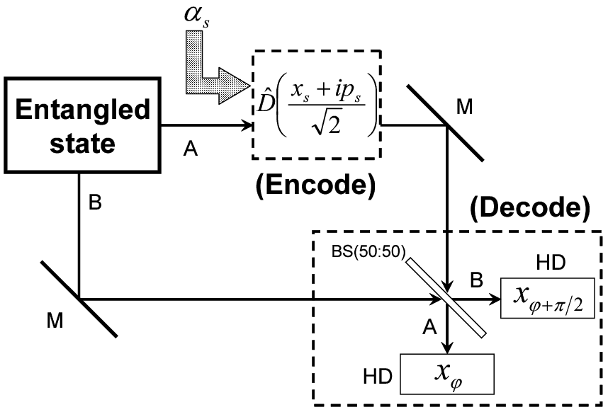
The second operational measure relates to the CV dense coding scheme Kitagawa05. The schematic is illustrated in Fig. 8.
Refer to caption
Figure 8: CV dense coding scheme scheme, with power of signal modulation αs\alpha_{s}. BS, M, and HD mean beam splitter, mirror, and homodyne detection, respectively.

In this scheme, Alice and Bob share the entangled state ρ^AB(E)\hat{\rho}_{\rm AB}^{\rm(E)} initially. Then, Alice encodes a classical message by a modulation on the beam path A,

U^A​(xs,ps)=e−(i/2)​xs​ps​D^​(xs+i​ps2)=e−i​ps​x^A​ei​xs​p^A,\hat{U}_{\rm A}(x_{s},p_{s})=e^{-(i/2)x_{s}p_{s}}\hat{D}\left(\frac{x_{s}+ip_{s}}{\sqrt{2}}\right)=e^{-ip_{s}\hat{x}_{\rm A}}e^{ix_{s}\hat{p}_{\rm A}}, (51)

where xsx_{s} and psp_{s} are related to the power of signal modulation αs\alpha_{s}. For the sake of simplicity, we consider the quaternary phase-shift keying (QPSK), with equal likelihood: a00=(xs=2​β,ps=2​β)a_{00}=(x_{s}=\sqrt{2}\beta,p_{s}=\sqrt{2}\beta), a01=(2​β,−2​β)a_{01}=(\sqrt{2}\beta,-\sqrt{2}\beta), a10=(−2​β,2​β)a_{10}=(-\sqrt{2}\beta,\sqrt{2}\beta), a11=(−2​β,−2​β)a_{11}=(-\sqrt{2}\beta,-\sqrt{2}\beta) for some real β\beta, and P⁡(ak​l)=1/4P(a_{kl})=1/4. Bob decodes the signals by the Bell measurement (40), and the decision rule is as follows: {b00=(x≥0,p≥0),b01=(x≥0,p<0),b10=(x<0,p≥0),b11=(x<0,p<0)}\{b_{00}=(x\geq 0,p\geq 0),b_{01}=(x\geq 0,p<0),b_{10}=(x<0,p\geq 0),b_{11}=(x<0,p<0)\}. The channel matrix of CV dense coding P(ch)​(bm​n|ak​l)P^{\rm(ch)}(b_{mn}|a_{kl}), whose elements are the conditional probabilities, is calculated with the homodyne probability distribution,

P(HD)(x,p|xs,ps)\displaystyle P^{\rm(HD)}(x,p|x_{s},p_{s})
=\displaystyle= ⟨Π(x,p)|U^A(xs,ps)ρ^AB(E)U^A†(xs,ps)|Π(x,p)⟩ABAB.\displaystyle{{}_{\rm AB}\langle}\Pi(x,p)|\hat{U}_{\rm A}(x_{s},p_{s})\hat{\rho}_{\rm AB}^{\rm(E)}\hat{U}_{\rm A}^{\dagger}(x_{s},p_{s})|\Pi(x,p)\rangle_{\rm AB}.

For example, P(ch)​(b00|a00)P^{\rm(ch)}(b_{00}|a_{00}) element of the channel matrix is

P(ch)(b00|a00)=∫0∞dx∫0∞dpP(HD)(x,p|2β,2β),P^{\rm(ch)}(b_{00}|a_{00})=\int_{0}^{\infty}dx\int_{0}^{\infty}dpP^{\rm(HD)}(x,p|\sqrt{2}\beta,\sqrt{2}\beta), (53)

and the other components are calculated similarly. With this 4×44\times 4 channel matrix, the mutual information is calculated as

I⁡(A;B)\displaystyle I(\textrm{A;B}) =\displaystyle= ∑k,l,m,nP⁡(ak​l)​P(ch)​(bm​n|ak​l)\displaystyle\sum_{k,l,m,n}P(a_{kl})P^{\rm(ch)}(b_{mn}|a_{kl})
×log2⁡[P(ch)​(bm​n|ak​l)∑k′,l′P⁡(ak′​l′)​P(ch)​(bm​n|ak′​l′)]​[bit].\displaystyle\times\log_{2}\left[\frac{P^{\rm(ch)}(b_{mn}|a_{kl})}{\sum_{k^{\prime},l^{\prime}}P(a_{k^{\prime}l^{\prime}})P^{\rm(ch)}(b_{mn}|a_{k^{\prime}l^{\prime}})}\right]\ \textrm{[bit]}.

With the two-mode squeezed vacuum state (3),

ISQ​(A;B)\displaystyle I_{\rm SQ}(\textrm{A;B})
=[1+erf​(1+λ1−λ​β)]​log2​[1+erf​(1+λ1−λ​β)]\displaystyle=\left[1+\textrm{erf}\left(\sqrt{\frac{1+\lambda}{1-\lambda}}\beta\right)\right]\log_{2}\left[1+\textrm{erf}\left(\sqrt{\frac{1+\lambda}{1-\lambda}}\beta\right)\right]
+[1−erf​(1+λ1−λ​β)]​log2​[1−erf​(1+λ1−λ​β)],\displaystyle+\left[1-\textrm{erf}\left(\sqrt{\frac{1+\lambda}{1-\lambda}}\beta\right)\right]\log_{2}\left[1-\textrm{erf}\left(\sqrt{\frac{1+\lambda}{1-\lambda}}\beta\right)\right],

where

erf​(x)=2π​∫0xd​t​e−t2\textrm{erf}(x)=\frac{2}{\sqrt{\pi}}\int_{0}^{x}dte^{-t^{2}} (56)

is the error function. With the non-Gaussian pure state (11),

ING(1)​(A;B)\displaystyle I_{\rm NG}^{(1)}(\textrm{A;B}) =\displaystyle= 14​(I1​log2​I1+I2​log2​I2CLOSE\displaystyle\frac{1}{4}(I_{1}\log_{2}I_{1}+I_{2}\log_{2}I_{2} (57)
OPEN+I3​log2​I3+I4​log2​I4),\displaystyle\hskip 28.45274pt+I_{3}\log_{2}I_{3}+I_{4}\log_{2}I_{4}),

and

I1\displaystyle I_{1} =\displaystyle= 𝒟μ​1μ​[1+erf​(1+λ​T1−λ​T​μ​β)]2|μ=1,\displaystyle\mathcal{D}_{\mu}\frac{1}{\mu}\left[1+\textrm{erf}\left(\sqrt{\displaystyle\frac{1+\lambda T}{1-\lambda T}\mu}\beta\right)\right]^{2}\Bigg|_{\mu=1}, (58)
I2=I3\displaystyle I_{2}=I_{3} =\displaystyle= 𝒟μ​1μ​[1−erf​(1+λ​T1−λ​T​μ​β)2]|μ=1,\displaystyle\mathcal{D}_{\mu}\frac{1}{\mu}\left[1-\textrm{erf}\left(\sqrt{\displaystyle\frac{1+\lambda T}{1-\lambda T}\mu}\beta\right)^{2}\right]\Bigg|_{\mu=1}, (59)
I4\displaystyle I_{4} =\displaystyle= 𝒟μ​1μ​[1−erf​(1+λ​T1−λ​T​μ​β)]2|μ=1,\displaystyle\mathcal{D}_{\mu}\frac{1}{\mu}\left[1-\textrm{erf}\left(\sqrt{\displaystyle\frac{1+\lambda T}{1-\lambda T}\mu}\beta\right)\right]^{2}\Bigg|_{\mu=1}, (60)

where

𝒟μ\displaystyle\mathcal{D}_{\mu} =\displaystyle= (1−λ2)​λ2​T2Pdet(1)​(1−λ​T)2​(1−λ2​T2)​(RT)2\displaystyle\frac{(1-\lambda^{2})\lambda^{2}T^{2}}{P_{\rm det}^{(1)}(1-\lambda T)^{2}(1-\lambda^{2}T^{2})}\left(\frac{R}{T}\right)^{2} (61)
×[(λ​T1+λ​T)2​∂2∂μ2+2​λ​T1+λ​T​∂∂μ+1],\displaystyle\times\left[\left(\frac{\lambda T}{1+\lambda T}\right)^{2}\frac{\partial^{2}}{\partial\mu^{2}}+\frac{2\lambda T}{1+\lambda T}\frac{\partial}{\partial\mu}+1\right],

containing the differential operation with respect to the auxiliary parameter μ\mu. With the non-Gaussian mixed state (14),

ℐNG​(A;B)\displaystyle\mathcal{I}_{\rm NG}(\textrm{A;B}) =\displaystyle= 14​(ℐ1​log2​ℐ1+ℐ2​log2​ℐ2CLOSE\displaystyle\frac{1}{4}(\mathcal{I}_{1}\log_{2}\mathcal{I}_{1}+\mathcal{I}_{2}\log_{2}\mathcal{I}_{2} (62)
OPEN+ℐ3​log2​ℐ3+ℐ4​log2​ℐ4),\displaystyle\hskip 28.45274pt+\mathcal{I}_{3}\log_{2}\mathcal{I}_{3}+\mathcal{I}_{4}\log_{2}\mathcal{I}_{4}),

where

ℐ1\displaystyle\mathcal{I}_{1} =\displaystyle= ∑i,j=01(−1)i+j​𝒞i​j​[1+erf​(Ωi​j​β)]2,\displaystyle\sum_{i,j=0}^{1}(-1)^{i+j}\mathcal{C}_{ij}\left[1+\textrm{erf}(\Omega_{ij}\beta)\right]^{2}, (63)
ℐ2=ℐ3\displaystyle\mathcal{I}_{2}=\mathcal{I}_{3} =\displaystyle= ∑i,j=01(−1)i+j​𝒞i​j​[1−erf​(Ωi​j​β)2],\displaystyle\sum_{i,j=0}^{1}(-1)^{i+j}\mathcal{C}_{ij}\left[1-\textrm{erf}(\Omega_{ij}\beta)^{2}\right], (64)
ℐ4\displaystyle\mathcal{I}_{4} =\displaystyle= ∑i,j=01(−1)i+j​𝒞i​j​[1−erf​(Ωi​j​β)]2,\displaystyle\sum_{i,j=0}^{1}(-1)^{i+j}\mathcal{C}_{ij}\left[1-\textrm{erf}(\Omega_{ij}\beta)\right]^{2}, (65)

and

𝒞i​j\displaystyle\mathcal{C}_{ij} =\displaystyle= 14​𝒫det​1−λ21−λ2​(T+γi)​(T+γj),\displaystyle\frac{1}{4\mathcal{P}_{\rm det}}\frac{1-\lambda^{2}}{1-\lambda^{2}(T+\gamma_{i})(T+\gamma_{j})}, (66)
Ωi​j\displaystyle\Omega_{ij} =\displaystyle= 1−λ2​(T+γi)​(T+γj)(1−λ​T)2−λ2​γi​γj,\displaystyle\sqrt{\frac{1-\lambda^{2}(T+\gamma_{i})(T+\gamma_{j})}{(1-\lambda T)^{2}-\lambda^{2}\gamma_{i}\gamma_{j}}}, (67)

where γ1=R\gamma_{1}=R and γ0=0\gamma_{0}=0 as before. See appendices A and B for more detailed derivations.

In the limit as T→1T\rightarrow 1, ℐNG​(A;B)=ING(1)​(A;B)\mathcal{I}_{\rm NG}(\textrm{A;B})=I_{\rm NG}^{(1)}(\textrm{A;B}) which has no intersection with ISQ​(A;B)I_{\rm SQ}(\textrm{A;B}) unless λ=0\lambda=0, therefore

ISQ​(A;B)≤limT→1ING(1)​(A;B).I_{\rm SQ}(\textrm{A;B})\leq\lim_{T\rightarrow 1}I_{\rm NG}^{(1)}(\textrm{A;B}). (68)

For T<1T<1, however, above inequality cannot hold for larger λ\lambda. In Figs. 9 and 10, the mutual information with the photon-subtracted squeezed states (T=0.9T=0.9) and the squeezed vacuum state are shown, at β=1.5\beta=1.5 and 0.7, respectively.

Refer to caption
Figure 9: Mutual information in dense coding scheme with the photon-subtracted pure state (dashed line), mixed one (solid line), and squeezed vacuum state (dotted line) at β=1.5\beta=1.5.
Refer to caption
Figure 10: The same plot as Fig. 9 at β=0.7\beta=0.7.

From these results, we can see that the range of λ\lambda for which the non-Gaussian operation brings the gain to the mutual information becomes wide as β\beta becomes small. When β\beta gets smaller, the overlap between the probability distributions of different signals increases, and the distinction of encoded signals becomes more difficult. In this situation, we can see the bona fide effect of entanglement in CV dense coding scheme. As β→0\beta\rightarrow 0, the intersections of the curves for the non-Gaussian states and the squeezed vacuum state approach λDP≃0.894\lambda_{\rm D}^{\rm P}\simeq 0.894 and λDM≃0.762\lambda_{\rm D}^{\rm M}\simeq 0.762, respectively (Fig. 11).

Refer to caption
Figure 11: Intersections of the input squeezed state curve and photon-subtracted squeezed state curves. It converges to λDP≃0.894\lambda_{\rm D}^{\rm P}\simeq 0.894 for the pure state case, and λDM≃0.762\lambda_{\rm D}^{\rm M}\simeq 0.762 for mixed one, as β→0\beta\rightarrow 0.

These intersections are quite close to those of the logarithmic negativity. This is consistent with the logarithmic negativity result in the sense that the mutual information indicates the range for which non-Gaussian operation enhances the entanglement.

VI Discussion and conclusion

In this paper, we have studied how to quantify the entanglement of the non-Gaussian mixed state which is generated by the photon subtraction from the two-mode squeezed vacuum state. In order to enhance the entanglement of a Gaussian state, shared by spatially-separated parties, using LOCC, then non-Gaussian operations are necessary. When the photon subtraction is carried out using on/off detectors, the resulting state is generally a mixed state. Evaluating the entanglement of such a state is far from trivial.

We have applied the negativity and the logarithmic negativity, which are known to be entanglement monotones, to this problem. We have compared the gain in terms of these measures with the one in terms of certain protocol-specific operational measures, namely the teleportation fidelity and the mutual information of the dense coding.

In the asymptotic limit T→1T\rightarrow 1, one would have an ideal single photon subtraction even with on/off detector and hence have an pure non-Gaussian state, although the successful probability of event selection approaches zero. This ideal non-Gaussian state is always superior to the input squeezed vacuum state for all the measures. For T<1T<1, on the other hand, up to a certain point of λ\lambda, the photon-subtracted squeezed states, both the pure and mixed states, are superior to the input squeezed state with respect to all the measures. Exceeding this point λ\lambda, the non-Gaussian operation brings no gain, and the entangled squeezed state shows the better performance. When λ\lambda approaches unity, the effect of the non-Gaussian operation for entanglement enhancement gets lost. This is because the initial squeezed state approaches the maximally entangled EPR state, as λ→1{\lambda}{\rightarrow}1, whose entanglement cannot be enhanced by any physical process.

While the operational measures have clear physical meanings, they directly depend on the input state characteristics, and the evaluation based on them vary for the protocols. The (logarithmic) negativity is, on the other hand, independent of any such external parameters. This quantity reflects the entanglement as an intrinsic property of the state of interest, namely the final output state. We have found that whenever the enhancement is seen in terms of the operational measures, the negativity and the logarithmic negativity are also enhanced. For the dense coding scheme, in particular, the upper limit of λ\lambda below which the non-Gaussian operational gain can be seen, λDP\lambda_{\rm D}^{\rm P} (pure state case) and λDM\lambda_{\rm D}^{\rm M} (mixed state case) approach the ones measured by the logarithmic negativity λLNP\lambda_{\rm LN}^{\rm P} and λLNM\lambda_{\rm LN}^{\rm M}, respectively, as the modulation signal power β\beta gets smaller. It would be interesting to investigate whether the intersections λD\lambda_{\rm D} in the dense coding as well as λT\lambda_{\rm T} for the teleportation are identical to λLN\lambda_{\rm LN} or not after the operational measures are further optimized with respect to all the possibilities for external parameters of input states. In other words, the logarithmic negativity, not containing any additional parameter, might give the universal upper limit for the region of λ\lambda, where the gain by the non-Gaussian operation can be seen.

The operational meaning of the logarithmic negativity has not completely been clear yet. The relationship between the logarithmic negativity and other entanglement measures, such as the entanglement of formation, has not yet been fully elucidated. Restricted to the case of symmetric Gaussian entangled states only, they always indicate the same ordering Adesso05. Generally, however, they could give the different ordering for a few cases Adesso05; Eisert99. Our findings will provide some insight into further studies of the evaluation of the performance of the non-Gaussian operations.

For practical application of our results to the laboratory experiment, various imperfections should be considered, such as the limited quantum efficiency and nonzero dark count rate of the photodetector, and linear loss in the optical paths. Then the logarithmic negativity evaluation in consideration of these imperfections is the important issue. However, those effects cause the complex mixing between two modes A and B. Therefore, it is not obvious whether the partially-transposed density matrix ρ^NGP​T\hat{\rho}^{PT}_{\rm NG} can be split into series of submatrices, as in the case of the ideal setup. This would make the analysis much harder even by numerical simulation. Such analysis for more practical situations is a future problem.

Acknowledgements.
The authors would like to M. Ban for valuable discussions.

Appendix A Derivation of () and (57)

Let us describe the non-Gaussian pure state in terms of coherent states, which is suitable for inner products with both the Fock state basis and continuous variable basis.

⟨n|α⟩\displaystyle\langle n|\alpha\rangle =\displaystyle= e−|α|22​αnn!,\displaystyle e^{-\frac{|\alpha|^{2}}{2}}\frac{\alpha^{n}}{\sqrt{n!}}, (69)
⟨x|α⟩\displaystyle\langle x|\alpha\rangle =\displaystyle= 1π4​exp⁡[−x22+2​x​α−α22−|α|22].\displaystyle\frac{1}{\sqrt[4]{\pi}}\exp\left[-\frac{x^{2}}{2}+\sqrt{2}x\alpha-\frac{\alpha^{2}}{2}-\frac{|\alpha|^{2}}{2}\right]. (70)

First, we consider the average fidelity of CV teleportation. With the coherent state basis, the non-Gaussian pure state (11) is expressed with an auxiliary parameter μ\mu,

|ψNG(1)⟩AB\displaystyle|\psi_{\rm NG}^{(1)}\rangle_{\rm AB} (71)
=\displaystyle= 1−λ2π2​Pdet(1)​∫d2​α​∫d2​β​R​α​β\displaystyle\frac{\sqrt{1-\lambda^{2}}}{\pi^{2}\sqrt{P_{\rm det}^{(1)}}}\int d^{2}\alpha\int d^{2}\beta R\alpha\beta
×exp⁡[−1+R2​(|α|2+|β|2)+λ​α∗​β∗]\displaystyle\times\exp\left[-\frac{1+R}{2}(|\alpha|^{2}+|\beta|^{2})+\lambda\alpha^{\ast}\beta^{\ast}\right]
|T​α⟩A​|T​β⟩B\displaystyle\hskip 85.35826pt|\sqrt{T}\alpha\rangle_{\rm A}|\sqrt{T}\beta\rangle_{\rm B}
=\displaystyle= R​1−λ2π2​Pdet(1)​∂∂μ​∫d2​α​∫d2​β\displaystyle\frac{R\sqrt{1-\lambda^{2}}}{\pi^{2}\sqrt{P_{\rm det}^{(1)}}}\frac{\partial}{\partial\mu}\int d^{2}\alpha\int d^{2}\beta
×exp⁡[−1+R2​(|α|2+|β|2)+λ​α∗​β∗+μ​α​β]\displaystyle\times\exp\left[-\frac{1+R}{2}(|\alpha|^{2}+|\beta|^{2})+\lambda\alpha^{\ast}\beta^{\ast}+\mu\alpha\beta\right]
|T​α⟩A​|T​β⟩B|μ=0,\displaystyle\hskip 85.35826pt|\sqrt{T}\alpha\rangle_{\rm A}|\sqrt{T}\beta\rangle_{\rm B}\Bigg|_{\mu=0},

where Pdet(1)P_{\rm det}^{(1)} is given by (12), and the auxiliary parameter μ\mu should be set to zero after all integration and differential operations. The inner product between the input state |α0⟩|\alpha_{0}\rangle and unnormalized output state after teleportation operation is

⟨α0|PNG(tlp)|ψout⟩BB\displaystyle{{}_{\rm B}\langle}\alpha_{0}|\sqrt{P_{\rm NG}^{\rm(tlp)}}|\psi_{\rm out}\rangle_{\rm B} (72)
=\displaystyle= ⟨α0|PNG(tlp)D^B(ξ)[⟨Π(x,p)|α0⟩TTA|ψNG(1)⟩AB]B\displaystyle{{}_{\rm B}\langle}\alpha_{0}|\sqrt{P_{\rm NG}^{\rm(tlp)}}\hat{D}_{\rm B}(\xi)\left[{{}_{\rm TA}\langle}\Pi(x,p)|\alpha_{0}\rangle_{\rm T}|\psi_{\rm NG}^{(1)}\rangle_{\rm AB}\right]
=\displaystyle= R​1−λ22​π​Pdet(1)​∂∂μ​11−λ​μ\displaystyle\frac{R\sqrt{1-\lambda^{2}}}{\sqrt{2\pi P_{\rm det}^{(1)}}}\frac{\partial}{\partial\mu}\frac{1}{1-\lambda\mu}
×exp⁡[−(1−λ​T1−λ​μ)​|Q|2+i2​x​p]|μ=0,\displaystyle\times\exp\left[-\left(1-\frac{\lambda T}{1-\lambda\mu}\right)\left|Q\right|^{2}+\frac{i}{2}xp\right]\Bigg|_{\mu=0},

where

Q=x+i​p2−α0=ξ−α0.Q=\frac{x+ip}{\sqrt{2}}-\alpha_{0}=\xi-\alpha_{0}. (73)

Therefore the (x,p)(x,p) component of the fidelity is

PNG(tlp)​FNG(1)​(x,p)\displaystyle P_{\rm NG}^{\rm(tlp)}F_{\rm NG}^{(1)}(x,p)
=\displaystyle= R2​(1−λ2)2​π​Pdet(1)​∂2∂μ1​∂μ2​1(1−λ​μ1)​(1−λ​μ2)\displaystyle\frac{R^{2}(1-\lambda^{2})}{2\pi P_{\rm det}^{(1)}}\frac{\partial^{2}}{\partial\mu_{1}\partial\mu_{2}}\frac{1}{(1-\lambda\mu_{1})(1-\lambda\mu_{2})}
×exp⁡[−(2−λ​T1−λ​μ1−λ​T1−λ​μ2)​|Q|2]|μ1=μ2=0.\displaystyle\times\exp\left[-\left(2-\frac{\lambda T}{1-\lambda\mu_{1}}-\frac{\lambda T}{1-\lambda\mu_{2}}\right)\left|Q\right|^{2}\right]\Bigg|_{\mu_{1}=\mu_{2}=0}.

By integrating Eq. () with respect to xx and pp, we obtain the average fidelity,

F¯NG(1)​(λ)\displaystyle\bar{F}_{\rm NG}^{(1)}(\lambda) (75)
=\displaystyle= ∫−∞∞d​x​∫−∞∞d​p​PNG(tlp)​FNG(1)​(x,p)\displaystyle\int_{-\infty}^{\infty}dx\int_{-\infty}^{\infty}dpP_{\rm NG}^{\rm(tlp)}F_{\rm NG}^{(1)}(x,p)
=\displaystyle= (1−λ2)​λ2​T2​(1−λ​T+λ2​T22)2​Pdet(1)​(1−λ​T)3​(RT)2,\displaystyle\frac{(1-\lambda^{2})\lambda^{2}T^{2}\left(1-\lambda T+\displaystyle\frac{\lambda^{2}T^{2}}{2}\right)}{2P_{\rm det}^{(1)}(1-\lambda T)^{3}}\left(\frac{R}{T}\right)^{2},

which is independent of the parameter α0\alpha_{0}.

Then, we consider the mutual information of CV dense coding channel.

⟨Π(x,p)|U^A(xs,ps)|ψNG(1)⟩ABABe−i​ps​(x−xs)\displaystyle{{}_{\rm AB}\langle}\Pi(x,p)|\hat{U}_{\rm A}(x_{s},p_{s})|\psi_{\rm NG}^{(1)}\rangle_{\rm AB}e^{-ip_{s}(x-x_{s})} (76)
=\displaystyle= 1−λ22​π5​Pdet(1)​∫d2​α​∫d2​β\displaystyle\sqrt{\frac{1-\lambda^{2}}{2\pi^{5}P_{\rm det}^{(1)}}}\int d^{2}\alpha\int d^{2}\beta
exp[−(|α|2+|β|2)+λα∗β∗+Tαβ\displaystyle\exp\Bigg[-(|\alpha|^{2}+|\beta|^{2})+\lambda\alpha^{\ast}\beta^{\ast}+T\alpha\beta
+Tξ′⁣∗α−Tξ′β−x22+ξ′22]Rαβ\displaystyle\hskip 28.45274pt+\sqrt{T}\xi^{\prime\ast}\alpha-\sqrt{T}\xi^{\prime}\beta-\frac{x^{2}}{2}+\frac{\xi^{\prime 2}}{2}\Bigg]R\alpha\beta
=\displaystyle= 1−λ22​π5​Pdet(1)​R​∂∂μ′​∫d2​α​∫d2​β\displaystyle\sqrt{\frac{1-\lambda^{2}}{2\pi^{5}P_{\rm det}^{(1)}}}R\frac{\partial}{\partial\mu^{\prime}}\int d^{2}\alpha\int d^{2}\beta
exp[−(|α|2+|β|2)+λα∗β∗+μ′αβ\displaystyle\exp\Bigg[-(|\alpha|^{2}+|\beta|^{2})+\lambda\alpha^{\ast}\beta^{\ast}+\mu^{\prime}\alpha\beta
+Tξ′⁣∗α−Tξ′β−x22+ξ′22]|μ′=T\displaystyle\hskip 28.45274pt+\sqrt{T}\xi^{\prime\ast}\alpha-\sqrt{T}\xi^{\prime}\beta-\frac{x^{2}}{2}+\frac{\xi^{\prime 2}}{2}\Bigg]\Bigg|_{\mu^{\prime}=T}
=\displaystyle= 1−λ22​π​Pdet(1)​RT​λ​T(1−λ​T)2​[−λ​T2​(1−λ​T)​|ξ′|2+1]\displaystyle\sqrt{\frac{1-\lambda^{2}}{2\pi P_{\rm det}^{(1)}}}\frac{R}{T}\frac{\lambda T}{(1-\lambda T)^{2}}\left[-\frac{\lambda T}{2(1-\lambda T)}|\xi^{\prime}|^{2}+1\right]
×exp⁡[−λ​T2​(1−λ​T)​|ξ′|2−(x−xs)22+ξ′22],\displaystyle\times\exp\left[-\frac{\lambda T}{2(1-\lambda T)}|\xi^{\prime}|^{2}-\frac{(x-x_{s})^{2}}{2}+\frac{\xi^{\prime 2}}{2}\right],

where we use the relation

U^A​(xs,ps)​|Π⁡(x,p)⟩AB=e−i​ps​(x−xs)​|Π⁡(x−xs,p−ps)⟩AB,\hat{U}_{\rm A}(x_{s},p_{s})|\Pi(x,p)\rangle_{\rm AB}=e^{-ip_{s}(x-x_{s})}|\Pi(x-x_{s},p-p_{s})\rangle_{\rm AB}, (77)

and

ξ′=(x−xs)+i⁡(p−ps)2=ξ−ξs.\xi^{\prime}=\frac{(x-x_{s})+i(p-p_{s})}{\sqrt{2}}=\xi-\xi_{s}. (78)

The auxiliary parameter μ′(=μ+T)\mu^{\prime}(=\mu+T) should be set to TT after all integration and differential operations. From above, we obtain the homodyne probability distribution,

PNG(HD)(x,p|xs,ps)\displaystyle P_{\rm NG}^{\rm(HD)}(x,p|x_{s},p_{s}) (79)
=\displaystyle= |⟨Π(x,p)|U^A(xs,ps)|ψNG(1)⟩ABAB|2\displaystyle\left|{{}_{\rm AB}\langle}\Pi(x,p)|\hat{U}_{\rm A}(x_{s},p_{s})|\psi_{\rm NG}^{(1)}\rangle_{\rm AB}\right|^{2}
=\displaystyle= 1−λ22​π​Pdet(1)​λ2​T2(1−λ​T)4​(RT)2​[−λ​T2​(1−λ​T)​|ξ′|2+1]2\displaystyle\frac{1-\lambda^{2}}{2\pi P_{\rm det}^{(1)}}\frac{\lambda^{2}T^{2}}{(1-\lambda T)^{4}}\left(\frac{R}{T}\right)^{2}\left[-\frac{\lambda T}{2(1-\lambda T)}|\xi^{\prime}|^{2}+1\right]^{2}
×exp⁡[−1+λ​T2​(1−λ​T)​|ξ′|2]\displaystyle\hskip 28.45274pt\times\exp\left[-\frac{1+\lambda T}{2(1-\lambda T)}|\xi^{\prime}|^{2}\right]
=\displaystyle= 1−λ22​π​Pdet(1)​λ2​T2(1−λ​T)4​(RT)2\displaystyle\frac{1-\lambda^{2}}{2\pi P_{\rm det}^{(1)}}\frac{\lambda^{2}T^{2}}{(1-\lambda T)^{4}}\left(\frac{R}{T}\right)^{2}
[(λ​T1+λ​T)2​∂2∂μ′′2+2​λ​T1+λ​T​∂∂μ′′+1]\displaystyle\left[\left(\frac{\lambda T}{1+\lambda T}\right)^{2}\frac{\partial^{2}}{\partial\mu^{\prime\prime 2}}+\frac{2\lambda T}{1+\lambda T}\frac{\partial}{\partial\mu^{\prime\prime}}+1\right]
exp⁡[−μ′′​1+λ​T2​(1−λ​T)​|ξ′|2]|μ′′=1,\displaystyle\hskip 28.45274pt\exp\left[-\mu^{\prime\prime}\frac{1+\lambda T}{2(1-\lambda T)}|\xi^{\prime}|^{2}\right]\Bigg|_{\mu^{\prime\prime}=1},

where the auxiliary parameter μ′′\mu^{\prime\prime} should be set to unity after all differential operations. With Eq. (79), the components of channel matrix can be calculated. For example,

PNG(ch)​(b00|a00)\displaystyle P_{\rm NG}^{\rm(ch)}(b_{00}|a_{00})
=\displaystyle= ∫0∞dx∫0∞dpPNG(HD)(x,p|2β,2β)\displaystyle\int_{0}^{\infty}dx\int_{0}^{\infty}dpP_{\rm NG}^{\rm(HD)}(x,p|\sqrt{2}\beta,\sqrt{2}\beta)
=\displaystyle= 14​𝒟μ′′​1μ′′​[1+erf​(1+λ​T1−λ​T​μ′′​β)]2|μ′′=1,\displaystyle\frac{1}{4}\mathcal{D}_{\mu^{\prime\prime}}\frac{1}{\mu^{\prime\prime}}\left[1+\textrm{erf}\left(\sqrt{\frac{1+\lambda T}{1-\lambda T}\mu^{\prime\prime}}\beta\right)\right]^{2}\Bigg|_{\mu^{\prime\prime}=1},

where

𝒟μ′′\displaystyle\mathcal{D}_{\mu^{\prime\prime}} =\displaystyle= (1−λ2)​λ2​T2Pdet(1)​(1−λ​T)2​(1−λ2​T2)​(RT)2\displaystyle\frac{(1-\lambda^{2})\lambda^{2}T^{2}}{P_{\rm det}^{(1)}(1-\lambda T)^{2}(1-\lambda^{2}T^{2})}\left(\frac{R}{T}\right)^{2}
×[(λ​T1+λ​T)2​∂2∂μ′′2+2​λ​T1+λ​T​∂∂μ′′+1],\displaystyle\times\left[\left(\frac{\lambda T}{1+\lambda T}\right)^{2}\frac{\partial^{2}}{\partial\mu^{\prime\prime 2}}+\frac{2\lambda T}{1+\lambda T}\frac{\partial}{\partial\mu^{\prime\prime}}+1\right],

containing the differential operation with respect to the auxiliary parameter μ′′\mu^{\prime\prime}. Other components can be derived similarly. With these results, we can obtain the mutual information (57).

Appendix B Derivation of (48) and (62)

Similar to the Appendix A, we describe the non-Gaussian mixed state with coherent basis,

ρ^NG\displaystyle\hat{\rho}_{\rm NG} (82)
=\displaystyle= 1−λ2π4​𝒫det​∫d2​α1​∫d2​α2​∫d2​β1​∫d2​β2\displaystyle\frac{1-\lambda^{2}}{\pi^{4}\mathcal{P}_{\rm det}}\int d^{2}\alpha_{1}\int d^{2}\alpha_{2}\int d^{2}\beta_{1}\int d^{2}\beta_{2}
exp[−1+R2(|α1|2+|α2|2+|β1|2+|β2|2)\displaystyle\exp\bigg[-\frac{1+R}{2}(|\alpha_{1}|^{2}+|\alpha_{2}|^{2}+|\beta_{1}|^{2}+|\beta_{2}|^{2})
+λ(α1∗β1∗+α2β2)]\displaystyle\hskip 113.81102pt+\lambda(\alpha_{1}^{\ast}\beta_{1}^{\ast}+\alpha_{2}\beta_{2})\bigg]
×(eR⁡(α1​α2∗+β1​β2∗)−eR​α1​α2∗−eR​β1​β2∗+1)\displaystyle\times\left(e^{R(\alpha_{1}\alpha_{2}^{\ast}+\beta_{1}\beta_{2}^{\ast})}-e^{R\alpha_{1}\alpha_{2}^{\ast}}-e^{R\beta_{1}\beta_{2}^{\ast}}+1\right)
|T​α1⟩A​⟨T​α2|⊗|T​β1⟩B​⟨T​β2|\displaystyle\hskip 28.45274pt|\sqrt{T}\alpha_{1}\rangle_{\rm A}\langle\sqrt{T}\alpha_{2}|\otimes|\sqrt{T}\beta_{1}\rangle_{\rm B}\langle\sqrt{T}\beta_{2}|
=\displaystyle= ∑i,j=01(−1)i+j​1−λ2π4​𝒫det​∫d2​α1​∫d2​α2​∫d2​β1​∫d2​β2\displaystyle\sum_{i,j=0}^{1}(-1)^{i+j}\frac{1-\lambda^{2}}{\pi^{4}\mathcal{P}_{\rm det}}\int d^{2}\alpha_{1}\int d^{2}\alpha_{2}\int d^{2}\beta_{1}\int d^{2}\beta_{2}
exp[−1+R2(|α1|2+|α2|2+|β1|2+|β2|2)\displaystyle\exp\bigg[-\frac{1+R}{2}(|\alpha_{1}|^{2}+|\alpha_{2}|^{2}+|\beta_{1}|^{2}+|\beta_{2}|^{2})
+λ(α1∗β1∗+α2β2)+γiα1α2∗+γjβ1β2∗]\displaystyle\hskip 14.22636pt+\lambda(\alpha_{1}^{\ast}\beta_{1}^{\ast}+\alpha_{2}\beta_{2})+\gamma_{i}\alpha_{1}\alpha_{2}^{\ast}+\gamma_{j}\beta_{1}\beta_{2}^{\ast}\bigg]
|T​α1⟩A​⟨T​α2|⊗|T​β1⟩B​⟨T​β2|,\displaystyle\hskip 28.45274pt|\sqrt{T}\alpha_{1}\rangle_{\rm A}\langle\sqrt{T}\alpha_{2}|\otimes|\sqrt{T}\beta_{1}\rangle_{\rm B}\langle\sqrt{T}\beta_{2}|,

where 𝒫det\mathcal{P}_{\rm det} is give by Eq. (16), and γ1=R\gamma_{1}=R, γ0=0\gamma_{0}=0.

With the representation (82), the unnormalized state after teleportation operation is

𝒫NG(tlp)​(x,p)​ρ^NG(out)​(x,p)\displaystyle\mathcal{P}^{\rm(tlp)}_{\rm NG}(x,p)\hat{\rho}_{\rm NG}^{\rm(out)}(x,p) (83)
=\displaystyle= D^B(ξ)⟨Π(x,p)|[ρ^T(in)⊗ρ^AB(E)]|Π(x,p)⟩TATAD^B†(ξ),\displaystyle\hat{D}_{\rm B}(\xi){{}_{\rm TA}\langle}\Pi(x,p)|\Big[\hat{\rho}_{\rm T}^{\rm(in)}\otimes\hat{\rho}_{\rm AB}^{\rm(E)}\Big]|\Pi(x,p)\rangle_{\rm TA}\hat{D}_{\rm B}^{\dagger}(\xi),
=\displaystyle= ∑i,j=01(−1)i+j​1−λ22​π3​𝒫det​∫d2​β1​∫d2​β2\displaystyle\sum_{i,j=0}^{1}(-1)^{i+j}\frac{1-\lambda^{2}}{2\pi^{3}\mathcal{P}_{\rm det}}\int d^{2}\beta_{1}\int d^{2}\beta_{2}
exp[−1+R2(|β1|2+|β2|2)+γjβ1β2∗+λ2γiβ1∗β2\displaystyle\exp\bigg[-\frac{1+R}{2}(|\beta_{1}|^{2}+|\beta_{2}|^{2})+\gamma_{j}\beta_{1}\beta_{2}^{\ast}+\lambda^{2}\gamma_{i}\beta_{1}^{\ast}\beta_{2}
−λ​T​Q​β1∗−λ​T​Q∗​β2−|Q|2\displaystyle\hskip 28.45274pt-\lambda\sqrt{T}Q\beta_{1}^{\ast}-\lambda\sqrt{T}Q^{\ast}\beta_{2}-|Q|^{2}
+T2(ξβ1∗−ξ∗β1+ξ∗β2−ξβ2∗)]\displaystyle\hskip 56.9055pt+\frac{\sqrt{T}}{2}(\xi\beta_{1}^{\ast}-\xi^{\ast}\beta_{1}+\xi^{\ast}\beta_{2}-\xi\beta_{2}^{\ast})\bigg]
|T​β1+ξ⟩B​⟨T​β2+ξ|,\displaystyle\hskip 85.35826pt|\sqrt{T}\beta_{1}+\xi\rangle_{\rm B}\langle\sqrt{T}\beta_{2}+\xi|,

where QQ and ξ\xi are similar to the definition in Eq. (73). Therefore, the (x,p)(x,p) component of the fidelity is

𝒫NG(tlp)​(x,p)​ℱNG​(x,p)\displaystyle\mathcal{P}_{\rm NG}^{\rm(tlp)}(x,p)\mathcal{F}_{\rm NG}(x,p)
=\displaystyle= ∑i,j=01(−1)i+j​12​π​𝒫det​1−λ21−λ2​γi​γj\displaystyle\sum_{i,j=0}^{1}(-1)^{i+j}\frac{1}{2\pi\mathcal{P}_{\rm det}}\frac{1-\lambda^{2}}{1-\lambda^{2}\gamma_{i}\gamma_{j}}
×exp⁡[−𝒦i​j​{(x−2​α0(r))2+(p−2​α0(i))2}],\displaystyle\times\exp\left[-\mathcal{K}_{ij}\left\{\left(x-\sqrt{2}\alpha_{0}^{\rm(r)}\right)^{2}+\left(p-\sqrt{2}\alpha_{0}^{\rm(i)}\right)^{2}\right\}\right],

where

𝒦i​j=1−λ​T−λ2​γi​γj−λ2​T2​(γi+γj)1−λ2​γi​γj\mathcal{K}_{ij}=\frac{1-\lambda T-\lambda^{2}\gamma_{i}\gamma_{j}-\frac{\lambda^{2}T}{2}(\gamma_{i}+\gamma_{j})}{1-\lambda^{2}\gamma_{i}\gamma_{j}} (85)

and α0=α0(r)+i​α0(i)\alpha_{0}=\alpha_{0}^{\rm(r)}+i\alpha_{0}^{\rm(i)}.

By integrating Eq. () with respect to xx and pp, we obtain the average fidelity,

ℱ¯NG​(λ)\displaystyle\bar{\mathcal{F}}_{\rm NG}(\lambda) (86)
=\displaystyle= ∑i,j=01(−1)i+j​12​𝒫det​1−λ21−λ​T−λ2​γi​γj−λ2​T2​(γi+γj)\displaystyle\sum_{i,j=0}^{1}(-1)^{i+j}\frac{1}{2\mathcal{P}_{\rm det}}\frac{1-\lambda^{2}}{1-\lambda T-\lambda^{2}\gamma_{i}\gamma_{j}-\frac{\lambda^{2}T}{2}(\gamma_{i}+\gamma_{j})}
=\displaystyle= ∑i,j=01(−1)i+j​ℱi​j​(λ).\displaystyle\sum_{i,j=0}^{1}(-1)^{i+j}\mathcal{F}_{ij}(\lambda).

For the mutual information of dense coding, we calculate the homodyne probability distribution,

𝒫NG(HD)(x,p|xs,ps)\displaystyle\mathcal{P}^{\rm(HD)}_{\rm NG}(x,p|x_{s},p_{s}) (87)
=\displaystyle= ⟨Π(x,p)|U^A(xs,ps)ρ^NGU^A†(xs,ps)|Π(x,p)⟩ABAB\displaystyle{{}_{\rm AB}\langle}\Pi(x,p)|\hat{U}_{\rm A}(x_{s},p_{s})\hat{\rho}_{\rm NG}\hat{U}_{\rm A}^{\dagger}(x_{s},p_{s})|\Pi(x,p)\rangle_{\rm AB}
=\displaystyle= 12​π​𝒫det​1−λ2(1−λ​T)2−λ2​γi​γj\displaystyle\frac{1}{2\pi\mathcal{P}_{\rm det}}\frac{1-\lambda^{2}}{(1-\lambda T)^{2}-\lambda^{2}\gamma_{i}\gamma_{j}}
×exp⁡[−1−λ2​(T+γi)​(T+γj)2​{(1−λ​T)2−λ2​γi​γj}​|ξ′|2]\displaystyle\times\exp\left[-\frac{1-\lambda^{2}(T+\gamma_{i})(T+\gamma_{j})}{2\{(1-\lambda T)^{2}-\lambda^{2}\gamma_{i}\gamma_{j}\}}|\xi^{\prime}|^{2}\right]
=\displaystyle= ∑i,j=01(−1)i+j𝒫i​j(x,p|xs,ps),\displaystyle\sum_{i,j=0}^{1}(-1)^{i+j}\mathcal{P}_{ij}(x,p|x_{s},p_{s}),

where ξs\xi_{s} and ξ′\xi^{\prime} are given in Eq. (78).

With (87), the component of channel matrix can be calculated. For example,

𝒫NG(ch)​(b00|a00)\displaystyle\mathcal{P}^{\rm(ch)}_{\rm NG}(b_{00}|a_{00}) (88)
=\displaystyle= ∫0∞dx∫0∞dp𝒫NG(ch)(x,p|2β,2β)\displaystyle\int_{0}^{\infty}dx\int_{0}^{\infty}dp\mathcal{P}^{\rm(ch)}_{\rm NG}(x,p|\sqrt{2}\beta,\sqrt{2}\beta)
=\displaystyle= ∑i,j=01(−1)i+j4​𝒫det​1−λ21−λ2​(T+γi)​(T+γj)\displaystyle\sum_{i,j=0}^{1}\frac{(-1)^{i+j}}{4\mathcal{P}_{\rm det}}\frac{1-\lambda^{2}}{1-\lambda^{2}(T+\gamma_{i})(T+\gamma_{j})}
×[1+erf​(1−λ2​(T+γi)​(T+γj)(1−λ​T)2−λ2​γi​γj​β)]2\displaystyle\times\left[1+\textrm{erf}\left(\sqrt{\frac{1-\lambda^{2}(T+\gamma_{i})(T+\gamma_{j})}{(1-\lambda T)^{2}-\lambda^{2}\gamma_{i}\gamma_{j}}}\beta\right)\right]^{2}
=\displaystyle= ∑i,j=01(−1)i+j​𝒞i​j​[1+erf​(Ωi​j​β)]2.\displaystyle\sum_{i,j=0}^{1}(-1)^{i+j}\mathcal{C}_{ij}\left[1+\textrm{erf}\left(\Omega_{ij}\beta\right)\right]^{2}.

Other components can be derived similarly. With these results, we can obtain the mutual information (62).

References

  • (1) M. A. Nielsen and I. L. Chuang, Quantum Computation and Quantum Information (Cambridge University Press, Cambridge, 2000).
  • (2) S. L. Braunstein and A. K. Pati, Quantum Information with Continuous Variables (Kluwer Academic Publishers, Dordrecht, 2003).
  • (3) S. L. Braunstein and H. J. Kimble, Phys. Rev. Lett. 80, 869 (1998); L. Vaidman, Phys. Rev. A 49, 1473 (1994).
  • (4) A. Furusawa, J. L. Sørensen, S. L. Braunstein, C. A. Fuchs, H. J. Kimble, and E. S. Polzik, Science 282, 706 (1998).
  • (5) T. C. Zhang, K. W. Goh, C. W. Chou, P. Lodahl, and H. J. Kimble, Phys. Rev. A 67, 033802 (2003).
  • (6) W. P. Bowen, N. Treps, B. C. Buchler, R. Schnabel, T. C. Ralph, Hans-A. Bachor, T. Symul, and P. K. Lam, ibid 67, 032302 (2003).
  • (7) M. Ban, J. Opt. B: Quantum Semiclass Opt. 1, L9 (1999); S. L. Braunstein and H. J. Kimble, Phys. Rev. A 61, 042302 (2000).
  • (8) X. Li, Q. Pan, J. Jing, J. Zhang, C. Xie, and K. Peng, Phys. Rev. Lett. 88, 047904 (2002).
  • (9) J. Mizuno, K. Wakui, A. Furusawa, and M. Sasaki, Phys. Rev. A 71, 012304 (2005).
  • (10) X. Jia, X. Su, Q. Pan, J. Gao, C. Xie, and K. Peng, Phys. Rev. Lett. 93, 250503 (2004).
  • (11) N. Takei, H. Yonezawa, T. Aoki, and A. Furusawa, Phys. Rev. Lett. 94, 220502 (2005).
  • (12) J. Eisert, S. Scheel, and M. B. Plenio, Phys. Rev. Lett. 89, 137903 (2002).
  • (13) J. Fiurášek, Phys. Rev. Lett. 89, 137904 (2002).
  • (14) G. Giedke and J. I. Cirac, Phys. Rev. A 66, 032316 (2002).
  • (15) D. Gottesman, A. Kitaev, and J. Preskill, Phys. Rev. A 64, 012310 (2001).
  • (16) K. Nemoto and W. J. Munro, Phys. Rev. Lett. 93, 250502 (2004).
  • (17) T. Opatrný, G. Kurizki, and D.-G. Welsch, Phys. Rev. A 61, 032302 (2000).
  • (18) P. T. Cochrane, T. C. Ralph, and G. J. Milburn, Phys. Rev. A 65, 062306 (2002).
  • (19) D. E. Browne, J. Eisert, S. Scheel, and M. B. Plenio, Phys. Rev. A 67, 062320 (2003).
  • (20) S. Olivares, M. G. A. Paris, and R. Bonifacio, Phys. Rev. A 67, 032314 (2003).
  • (21) H. Nha and H. J. Carmichael, Phys. Rev. Lett. 93, 020401 (2004).
  • (22) R. Garcia-Patrón, J. Fiurášek, N. J. Cerf, J. Wenger, R. Tualle-Brouri, and Ph. Grangier, Phys. Rev. Lett. 93, 130409 (2004); R. Garcia-Patrón, J. Fiurášek, and N. J. Cerf, Phys. Rev. A 71, 022105 (2005).
  • (23) S. Olivares and M. G. A. Paris, Phys. Rev. A 70, 032112 (2004).
  • (24) A. Kitagawa, M. Takeoka, K. Wakui, and M. Sasaki, Phys. Rev. A 72, 022334 (2005).
  • (25) G. Vidal, J. Mod. Opt. 47, 355 (2000).
  • (26) C. H. Bennett, D. P. DiVincenzo, J. A. Smolin, and W. K. Wootters, Phys. Rev. A 54, 3824 (1996).
  • (27) W. K. Wootters, Phys. Rev. Lett. 80, 2245 (1998).
  • (28) P. M. Hayden, M. Horodecki, and B. M. Terhal, J. Phys. A: Math. Gen. 34, 6891 (2001).
  • (29) V. Vedral and M. B. Plenio, Phys. Rev. A 57, 1619 (1998).
  • (30) G. Vidal and R. F. Werner, Phys. Rev. A 65, 032314 (2002).
  • (31) A. Peres, Phys. Rev. Lett. 77, 1413 (1996).
  • (32) M. Horodecki, P. Horodecki, and R. Horodecki, Phys. Rev. Lett. 84, 2014 (2000).
  • (33) M. B. Plenio and S. Virmani, arXiv:quant-ph/0504163.
  • (34) M. B. Plenio, Phys. Rev. Lett. 95, 090503 (2005).
  • (35) J. Eisert, Ph.D. thesis, University of Potsdam, 2001.
  • (36) G. Adesso and F. Illuminati, Phys. Rev. A 72, 032334 (2005).
  • (37) J. Eisert and M. B. Plenio, J. Mod. Opt. 46, 145 (1999).