Excitation and Entanglement Transfer Versus Spectral Gap

Most quantum information processing tasks require at some stage the transfer of quantum states between two quantum systems such as atoms or ions which are located a different positions in space. For transfer over long distances, photons sent through optical fibres seem promising. However the interactions between photons and the stationary systems, e.g. atoms, are weak and need to be controlled with high precision for transferring the state onto the photon and vice versa. Finding alternative methods and carriers is thus of considerable interest, in particular for transfer over short distances. Here, using condensed matter systems, e.g. a piece of solid, seems very appealing. Therefore the possibilities of transferring quantum information with strongly coupled quantum many body systems such as spin chains have been studied in some detail in recent years and several scenarios showing close to perfect state transfer have been found Bos03; PHE04.

One question arises naturally in this context: How do the properties of the employed many body system relate to the transfer quality and speed? A key property in this context is whether those systems feature an energetic gap between their ground state and excited states. Most interestingly, this gap vanishes at the critical points of quantum phase transitions Sachdev1999, where, at zero temperature, the ground state and an excited state exchange their roles as a parameter in the Hamiltonian, such as a magnetic field, is varied.

As with classical phase transitions, quantum phase transitions are usually analysed in terms of the scaling behaviour of equilibrium properties, where a diverging correlation length is indicative of a critical point Has; Sachdev1999; EC05. An analogous scaling phenomenon was recently also found for the entanglement properties of a spin chain in the vicinity of a quantum phase transition Osterloh2002; locent; JL05. Motivated by these findings and the recent experimental observation of the Mott quantum phase transition in the well-controlled environment of an optical lattice GME+02, the dynamical entanglement properties of quantum many body systems undergoing a quantum phase transition are receiving increasing attention. For example, one recent approach AUL05 was concerned with the dynamics of bipartite entanglement in spin chains resulting from an initial perturbation, while another studied the entanglement of two spins that are globally coupled to a quantum critical system YCW05. On another level, the Zurek-Kibble mechanism for classical phase transitions was recently generalised to its quantum analogue, further deepening our insight into the dynamics of quantum phase transitions ZDZ05.

In this article we study the relation between the size of the spectral gap of a quantum many body system and its capacity to transfer quantum information. Specifically, we study the transfer of quantum states for two examples of linear chains of interacting quantum systems. We employ newly developed matrix product state techniques Vid03 to simulate numerically the dynamics of spin chains exhibiting a quantum phase transition. Then we proceed to study a harmonic chain where we may choose the on-site potential such that the energy gap above the unique ground state vanishes. The latter of the two models allows us to obtain a better understanding of the relevant physics since it permits an analytical study in terms of master equations and the verification of the validity of the assumptions inherent in the master equation by numerically simulating the dynamics of the harmonic chain with up to $1400$ constituents PHE04.

We find that the transfer properties crucially depend on the energy gap between the ground state and the lowest excited states, but does not significantly dependent on the detailed structure of the Hamiltonian. In particular the transfer The characteristics of the state transfer through such systems may therefore be used to detect the critical point experimentally.

We begin by considering a 1-D chain of spins with nearest neighbour interactions and open boundary conditions. The Hamiltonian of our model reads

where $N$ is the number of spins, $B$ is an applied magnetic field and $J_{x}$, $J_{y}$ and $J_{z}$ the interaction between neighboring spins. Furthermore, two ancillas (named $S$ for “sender” and $R$ for “receiver”) couple to the chain at spins $m_{S}$ and $m_{R}$, which are near the centre of the chain in order to avoid boundary effects . The complete Hamiltonian is thus given by

$B_{a}\geq 0$ is the Zeeman splitting of the ancillas, which might differ from $B$, and $J_{a}\geq 0$ is the coupling of the ancillas to the chain, which is taken to be weak, i.e. $J_{a}\ll(B,J_{x},J_{y},J_{z})$. Figure 1 shows the topology of the model.

Initially, the chain is assumed to be in the ground state, $|0_{\textrm{chain}}\rangle$, of the Hamiltonian (1), while the sender is spin up and the receiver is spin down. Hence, the initial state of the total system is

We simulate the dynamics of our system numerically, making use of the recently introduced matrix product states Vid03. We use matrices of dimension $10\times 10$. To test the accuracy of our simulations, we verified whether the results where stable with respect to variations of the matrix dimension and the size of the timesteps. Furthermore, we tested whether the energy of the total system was conserved. Since the matrix product approximation can only be efficient if the considered system obeys a ”entropy and area law” PED+, which is not necessarily true at quantum critical points, our simulations consider only parameters near, but not exactly on the critical point.

Figure 2 shows the probability $P(\uparrow_{S}\downarrow_{R})$ that “sender” $S$ is in its excited state $|\uparrow_{S}\rangle$ and the “receiver” $R$ in its ground state $|\downarrow_{R}\rangle$, together with $P(\downarrow_{S}\uparrow_{R})$ and $P(\downarrow_{S}\downarrow_{R})$ for a model with $N=100$, $m_{S}=45$, $m_{R}=55$, $B=1$, $J_{x}=0.3$, $J_{y}=J_{z}=0$, $B_{a}=0.64$ and $J_{a}=0.05$. $P(\uparrow_{S}\uparrow_{R})$ is always less than $10^{-4}$.

The plots show that the excitation that was initially located in $S$ oscillates back and forth between $S$ and $R$.

Figure 3 shows $P(\uparrow_{S}\downarrow_{R})$, $P(\downarrow_{S}\uparrow_{R})$ and $P(\downarrow_{S}\downarrow_{R})$ for a model with $N=600$, $m_{S}=295$, $m_{R}=305$, $B=1$, $J_{x}=0.3$, $J_{y}=J_{z}=0$, $B_{a}=0.8$ and $J_{a}=0.05$. Again, $P(\uparrow_{S}\uparrow_{R})$ is always less than $10^{-4}$.

For these parameters, the excitation is not fully transferred to $R$, contrary to figure 2. Both, $S$ and $R$ relax to their ground states with the excitation only being partially and temporarily transferred to $R$, even for close-lying spins. Note that the parameters chosen in figures 2 and 3 are the same except for $B_{a}$ which in figure 3 is significantly larger than in figure 2.

The two observed scenarios are rather generic. To demonstrate this, we have done the same simulations for different parameters, i.e. for a XXZ-model. The results, shown in figures 4 and 5, clearly agree with our findings for the previous coupling parameters. Again $B_{a}$ in figure 5 is significantly larger than in figure 4, while all other parameters are equal.

The dramatic difference between the almost perfect transfer scenarios in figures 2 and 4 and the damped scenario in figures 3 and 5 has a simple physical explanation. The dynamics we have simulated is given by the Schrödinger equation containing the Hamiltonian (2). As a consequence, all moments of the Hamiltonian are conserved,

The initial state $|\Psi(0)\rangle$ is not an eigenstate of $H$ as given by (2), hence

where $E$ and $|E\rangle$ are the eigenvalues and eigenstates of $H$. However since a probability distribution is entirely determined by all moments, $\langle\Psi(t)|H^{n}|\Psi(t)\rangle=\kern 5.0pt$const for all $n$ implies $|\langle E|\Psi(t)\rangle|^{2}=|\langle E|\Psi(0)\rangle|^{2}$ for all $|E\rangle$. In other words the whole probability distribution given by the $|\langle E|\Psi(0)\rangle|^{2}$ is conserved. In our case, it’s variance is

For the dynamics this means that only those states with an energy expectation value $\overline{E}$ in the range $\langle\Psi(0)|H|\Psi(0)\rangle-2J_{a}<\overline{E}<\langle\Psi(0)|H|\Psi(0)\rangle+2J_{a}$ are accessible. Figure 6 sketches the energy levels of the system we consider. $S$ and $R$ are depicted as two level systems, while for the chain there is a unique ground state and a quasi continuous band of excited states sketched as the gray area. The dots indicate the initial occupations. The energy range which is accessible for the considered initial state lies between the two horizontal dashed lines. If the spectral gap is larger than the Zeeman splitting of the ancillas (left plot), there is no accessible excited state of the chain and hence no excitations get lost into the chain, which in turn implies the excitation will be almost completely transferred to $R$. If however the spectral gap is smaller than the Zeeman splitting of the ancillas, there are accessible excited states in the chain and excitation and hence quantum information get lost.

In order to obtain a more rigorous justification of this simple picture and to underline the generality of our findings, we now turn to a different model for the chain which also features an adjustable energy gap above its unique ground state.

We consider a harmonic chain with periodic boundary conditions (see fig. 7) described by

with the $p_{j}$ being the momenta and the $q_{j}$ the positions ($q_{N+1}=q_{1}$). In this case, the two ancillas are harmonic oscillators that couple to oscillators $m_{S}$ and $m_{R}$ of the chain. The complete Hamiltonian now reads

Since we are only interested in the time evolution of the ancillas, we derive a master equation for the dynamics of their reduced density matrix $\rho(t)$. For weak coupling $J_{a}\ll(\Omega,\Omega_{0})$, its equation of motion is given by

where $\sigma(t)$ and $H_{I}(t)$ are the density matrix of the ancillas and the interaction between ancillas and chain in the interaction picture, respectively: $H=H_{0}+H_{I}$ with $H_{0}=H_{\textrm{chain}}+H_{\textrm{ancillas}}$, $H_{I}(t)=\exp(iH_{0}t)H_{I}\exp(-iH_{0}t)$ and $\sigma(t)=\exp(iH_{0}t)\rho\exp(-iH_{0}t)$. $\textrm{Tr}_{\textrm{chain}}$ is the trace over the degrees of freedom of the chain and $|0\rangle$ denotes the ground state of the chain (7). The right hand side of eq. (11) is an expansion in the coupling strength $J_{a}$ up to second order, which is a good approximation if the integral approaches a constant value for $t>t^{\star}$, where $J_{a}t^{\star}\ll 1$. Since $\sigma$ only changes significantly on time scales $t\sim J_{a}^{-1}\gg t^{\star}$, the approximation $\sigma(s)\approx\sigma(t)$ can be used. Performing the trace on the rhs of (11) yields

where $a_{S}$ and $a_{R}$ are the annihilation operators of $S$ and $R$, respectively: $q_{j}=(a_{j}+a_{j}^{\dagger})/\sqrt{2\omega}$ and $p_{j}=-i(a_{j}-a_{j}^{\dagger})\sqrt{\omega/2}$ for $j=S,R$. $[\cdot,\cdot]$ and $\{\cdot,\cdot\}$ denote commutators and anti-commutators. On the rhs of the above equation, we neglected terms which contain two annihilation or two creation operators since they oscillate at high frequencies. The validity of this approximation can later be confirmed from the exact numerical solution. The coefficients read

with $C_{kl}^{\pm}$ given by

where $k,l=m_{S},m_{R}$. Due to the symmetries of the model, the $C_{kl}^{\pm}$ only depend on $|k-l|$, implying $C_{m_{S}m_{S}}^{\pm}=C_{m_{R}m_{R}}^{\pm}$ and $C_{m_{S}m_{R}}^{\pm}=C_{m_{R}m_{S}}^{\pm}$. Eq. (12) is a good approximation whenever

Since the $C_{kl}^{\pm}(t)$ do not depend on $J_{a}$ themselves, there is always a sufficiently small $J_{a}$ such that (18) holds, provided $\lim_{t\to\infty}C_{kl}^{\pm}(t)$ exists.

The harmonic chain can be diagonalised via a Fourier transform PHE04. In the limit of an infinitely long chain, $N\rightarrow\infty$, its dispersion relation is

and the correlation functions read

These expressions show, that indeed all $\lim_{t\to\infty}C_{kl}^{\pm}(t)$ exist except for the case where $\omega=\Omega_{0}=0$. As in master equations for system bath models, we now insert the asymptotic expressions

into eq. (12). This replacement assumes that all internal dynamics of the chain happens on much shorter time scales than the dynamics caused by the interaction of the ancillas with the chain. Furthermore, it does not treat the initial evolution for short times with full accuracy since $\lim_{t\to 0}C_{kl}^{\pm}(t)=0(\not=\overline{C}_{kl}^{\pm})$. The obtained master equation is thus valid in a regime where the couplings $J_{a}$ are weak enough such that the time it takes for an excitation to travel from $S$ to $R$ is completely determined by $J_{a}$, i.e. by the time it takes to be transferred into and from the chain. Consequently, the speed of sound of the chain is no longer resolved, and differences in the distance between $S$ and $R$ do not matter.

From eq. (12) we find the following solution for the expectation values of the occupation numbers of $S$ and $R$, $n_{S}=\textrm{Tr}(a_{S}^{\dagger}a_{S}\sigma)$ and $n_{R}=\textrm{Tr}(a_{R}^{\dagger}a_{R}\sigma)$:

Here, $A_{+}=\frac{n_{S}(0)+n_{R}(0)}{2}$, $A_{-}=\frac{n_{S}(0)-n_{R}(0)}{2}$, $x_{0}=\lim_{t\to\infty}X_{0}$, $x_{1}=\lim_{t\to\infty}X_{1}$ and $y_{1}=\lim_{t\to\infty}Y_{1}$. Note that $x_{0}>0$ and $x_{0}>|x_{1}|$.

Inserting the correlation functions into eq. (21) and using the relation

where $\mathcal{P}$ denotes the principal value of the subsequent integral, one sees that $x_{0}$ and $x_{1}$ are only non-zero if $\omega\geq\omega_{k}$ for at least one mode $k$, that is if our initial state is in resonance with (i.e. has the same energy expectation value as) states where both ancillas are in their ground states and the chain is in one of its lowest-lying excited states (c.f. figure 6). The dispersion relation shows that this only happens for $\omega\geq\Omega_{0}$. As in figures 2 and 3 or 4 and 5, we thus observe two different scenarios:

If $\omega<\Omega_{0}$, and therefore $x_{0}=x_{1}=0$, the excitation that is initially in $S$ oscillates back and forth between $S$ and $R$ at a frequency $2J_{a}^{2}y_{1}$, i.e.

Note in particular that the excitation is entirely transferred to $R$ at times $t_{n}=n(\pi/J_{a}^{2}y_{1});\>n=1,2,\dots$ . The solution (24) is plotted in figure 8 for a harmonic chain and ancillas with $\Omega=1$, $\omega=0.5$, $J_{a}=0.05$, $|m_{S}-m_{R}|=9$ and $\Omega_{0}=0.7$.

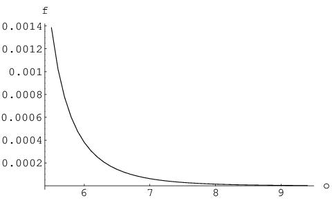
Figure 9 shows the frequencies $2J_{a}^{2}y_{1}$ of the excitation’s oscillations between $S$ and $R$ for cases where $\omega<\Omega_{0}$, for $\Omega=1$, $J_{a}=0.05$ and $\omega=0.35$ as a function of $\Omega_{0}$. As $\Omega_{0}-\omega$ decreases, the transfer becomes faster and the oscillation frequency increases.

If, on the other hand, $\omega\geq\Omega_{0}$, the chain acts similarly to a bath. Here, $x_{0}\not=0$, $x_{1}\not=0$, and both ancillas relax into their ground state transferring their energy into the chain. During this process, however, a fraction of the energy initially located in $S$ appears momentarily in $R$ before it is finally damped into the chain. The maximal excitation of the receiver throughout the entire evolution depends on the distance $|m_{S}-m_{R}|$. For a given initial energy in $S$, a narrow range of the excitation spectrum is relevant for the dynamics. The relation of the wavelength of these excitations to the distance $|m_{S}-m_{R}|$ determines the maximal transferred fraction of the excitation. Figure 10 shows the solution 22 for a harmonic chain and ancillas with $\Omega=1$, $\omega=0.5$, $J_{a}=0.05$, $|m_{S}-m_{R}|=9$ and $\Omega_{0}=0.2$.

One might try to derive the same type of master equation for the spin chain (1). However, for finite distances no exact expression for the time dependent correlation functions is known McC71. This is due to the fact that the subspaces of odd and of even number of fermions cannot be diagonalised simultaneously. An attempt of an approximation restricted to only one subspace led to reasonable results for some parameter values but occasionally produced unphysical solutions which grew exponentially in time. Therefore, such a master equation approach cannot be considered reliable for our spin chains and was avoided.

To confirm the validity of the master equation approach for the harmonic chain, we compared it to results of a numerical simulation of a chain with 1400 oscillators. Since the Hamiltonians of harmonic oscillators and harmonic chains are quadratic in the position and momentum operators, Gaussian states (states with a Gaussian Wigner function) remain Gaussian throughout the time evolution. For these states the complete dynamics can thus be obtained by only considering the evolution of the covariance matrix (see PHE04 for details). We found good agreement between our analytical and numerical solutions, with the relative errors being less than $5\%$.

The observed effects may also be formulated in quantum information language. In this way, one obtains statements on the average fidelity achieved for arbitrary input states (subspace fidelity) or the transfer of entanglement (entanglement fidelity), which are closely related Barnum KN 98. For the present setup, suppose there is an additional control spin $C$ which does not couple to the rest of the system, but is initially maximally entangled with $S$, see figure 11. A possible initial state is

The transfer of the entanglement across the chain may now be analysed by considering the entanglement between $R$ and $C$ as a function of time. Since we assume$J_{a}\ll(B,J_{x},J_{y},J_{z})$, the state $|\downarrow_{C},\downarrow_{S},\downarrow_{R},0\rangle$ is by virtue of energy conservation approximately stationary, while the evolution of $|\uparrow_{C},\uparrow_{S},\downarrow_{R},0\rangle$ is the same as above (modulo a phase). Since states with more than one excitation are energetically not accessible, the logarithmic negativity Ple05 for the reduced density matrix of $R$ and $C$ can be expressed approximately as

Hence, in this model $P(\downarrow_{S}\uparrow_{R})\approx 1$ implies that the entanglement has been transferred perfectly, too.

In conclusion, we have considered entanglement and excitation transfer through strongly coupled quantum many body systems. In particular we have studied the dependence of the transfer quality and speed on the size of the spectral gap between the ground and the lowest excited state of the considered system.

As a first main result, we find that the quality of transfer, and hence the quantum channel capacity, can be almost perfect whenever there is a finite, sufficiently large energy gap above the ground state. This opens up a generic way to design good quantum channels by using gapped systems, since the gap ensures high transfer quality irrespective of the system’s details.

On approaching quantum critical points, the spectral gap shrinks and the transfer decreases in quality, but accelerates. This second main result suggests a possible experimental determination of the energy gap: if one finds in an experiment that the energy is not completely transferred from one ancilla to the other, one can infer that the energy gap is smaller than the available energy. The bound can be made tighter by lowering the energy available in the “sender” ancilla. This procedure might in particular be helpful for cold atom systems in optical lattices, where standard spectroscopy is not applicable.

A quantitative study of the scaling of the transfer quality and time in between the two detected scenarios and its relation to critical exponents of various quantum phase transition universality classes Sachdev1999 should be a subject of future research. In that way an approach that originated in quantum information considerations might open up a new way to characterise and experimentally detect quantum phase transitions.

The authors would like to thank Sougato Bose and Daniel Burgarth for discussions at early stages of this project. This work is part of the QIP-IRC supported by EPSRC (GR/S82176/0), the Alexander von Humboldt Foundation, Hewlett-Packard and the EU Integrated Project QAP.

References

- (1) Sachdev S Quantum Phase Transitions. Cambridge Univ. Press, Cambridge, (1999).
- (2) Hastings M B Phys. Rev. Lett. 93, 126402 (2004); Hastings M B Phys. Rev. B 69, 104431 (2004); Hastings M B cond-mat/0508554 (2005); Hastings M B Phys. Rev. Lett. 93, 140402 (2004).
- (3) Cramer M, Eisert J, Plenio M B and Dreissig J. quant-ph/0505092 (2005); Cramer M and Eisert J. quant-ph/0509167 (2005); Wolf M M, Giedke G and Cirac J I. quant-ph/0509154 (2005).
- (4) Verstraete F, Martín-Delgado M A and Cirac J I. Phys. Rev. Lett. 92, 087201 (2004). Pachos J K and Plenio M B. Phys. Rev. Lett. 93, 056402 (2004); Kay A, Lee D K K, Pachos J K, Plenio M B, Reuter M E and Rico E. Optics and Spectroscopy 99, 355–372 (2005).
- (5) Osterloh A, Amico L, Falci G and Facio R. Nature 416, 608 (2002).
- (6) Larsson D and Johannesson H. Phys. Rev. Lett. 95, 196406 (2005).
- (7) Greiner M, Mandel O, Esslinger T, Hänsch T W and Bloch I. Nature 415, 39 (2002).
- (8) Sen A, Sen U and Lewenstein M. quant-ph/0505006 (2005).
- (9) Yi X X, Cui H T and Wang L C. quant-ph/0511026 (2005).
- (10) Zurek W H, Dorner U and Zoller P. cond-mat/0503511 (2005); Polkovnikov A. cond-mat/0312144 (2005); Dziarmaga J. cond-mat/0509490 (2005).
- (11) Bose S. Phys. Rev. Lett. 91, 207901 (2003); Burgarth D and Bose S. New J. Phys. 7, 135 2005.
- (12) Plenio M B, Hartley J, and Eisert J. New J. Phys. 6, 36 (2004); Eisert J, Plenio M B, Bose S, and Hartley J. Phys. Rev. Lett. 93, 190402 (2004); Plenio M B and Semião F. New J. Phys. 7, 73 (2005).
- (13) Vidal G. Phys. Rev. Lett. 93, 040502 (2004); Daley A J, Kollath C, Schollwoeck U and Vidal G. J. Stat. Mech.: Theor. Exp., P04005 (2004).
- (14) Plenio M B, Eisert J, Dreissig J, and Cramer M. Phys. Rev. Lett. 94, 060503 (2005).
- (15) Plenio M B. Phys. Rev. Lett. 95, 090503 (2005); Eisert J and Plenio M B. J. Mod. Opt. 46, 145 (1999); Eisert J. PhD thesis, University of Potsdam, February 2001; Vidal G and Werner R F. Phys. Rev. A 65, 032314 (2002); Audenaert K, Plenio M B and Eisert J. Phys. Rev. Lett. 90, 027901 (2003).
- (16) McCoy B M. Phys. Rev. A 4, 2331 (1971).
- (17) Barnum H, Knill E and Nielsen M A, quant-ph/9809010 (1998).