As a matter of principle, time-dependent density functional theory rungegross provides a highly efficient method to solve the time-dependent quantum many-body problem. It yields directly the time-dependent one-particle density $n(\vec{r},t)$ of the many-body system. All physical observables of the quantum system can, in principle, be determined from the density. In practice there a two essential ingredients to a TDDFT calculation. First an approximation to the time-dependent exchange-correlation potential $V_{xc}[n](\vec{r},t)$ has to be found which via the non-interacting Kohn-Sham system determines the evolution of the density. The second ingredient are functionals that allow the extraction of physical observables from the density. For some of the observables such as the ground-state energy extraction is straight forward within ground-state density functional theory hohenbergkohn. Excited-state spectra have been obtained from linear-response functionals casida; lr. Beyond linear response, the time-dependent dipole moment which governs the emission of high-harmonic radiation can be directly determined from $n(\vec{r},t)$. Ionization probabilities can be approximately extracted by identifying the integrated density beyond a certain critical distance from the bound system with the flux of ionized particles lappas; petersilka. However, in general, on the most fundamental level, state-to-state transition probabilities contain the full information on the response of a many-body system to an external perturbation. One example are bound-bound transition amplitudes required, e. g. in coherent control calculations of laser-matter interactions within TDDFT werschnik, currently a hot topic since atto-second laser pulses allow the control of the electron dynamics. This poses one fundamental question: How can state-to-state transition probabilities be extracted from TDDFT?
The ultimate goal of the study of the in general non-linear response of the many-body system to a time-dependent perturbation is the determination of the state-to-state transition amplitude

$$S_{if}=\lim_{t\to\infty}\langle\chi_{f}|U(t,-t)|\chi_{i}\rangle\,,$$

(1)

where $|\chi_{i,f}\rangle$ are the initial (final) channel states of the system prior to $(i)$ and after $(f)$ the perturbation, and $U(t_{1},t_{2})$ is the time evolution operator of the system. The challenge is, thus, to construct a functional $S_{i,f}[n]$ that allows to extract $S_{if}$ from TDDFT. The present paper addresses methods to extract transition probabilities between discrete states of the many-body system. As point of reference, we investigate first the evaluation of eq. (1) employing Kohn-Sham orbitals in close analogy to the time-dependent Hartree-Fock (TDHF) method (see bonche; griffin; alhassid; negele and references therein). This method would be the equivalent of the at least zeroth order of a time-dependent many-body perturbation theory ($S$-matrix theory) in which the time-dependent non-interacting Kohn-Sham system is considered as the unperturbed system. This method involves three steps of approximations: The initial state, the final state and the many-body propagator are approximated by their TDDFT equivalents. We encounter similar conceptual problems (“cross-channel correlations”) as TDHF does. We then formulate a novel functional that allows the determination of $S_{i,f}[n]$ which is shown to be free of these deficiencies. We test the method with the help of an exactly solvable two-electron model.
We consider an interacting $N$-electron system of Hamiltonian $H_{0}$ with stationary eigenstates $\chi_{i,f}$ which is subject to a perturbation $V(t)$ which is switched on at time $t=0$ and switched off at time $t=\tau$. The initial state of the system $|\chi_{i}\rangle$ is assumed to be the ground state and evolves according to the time-dependent many-body Schrödinger equation (in a.u.)

$$i\frac{\partial}{\partial t}|\Psi(t)\rangle=[H_{0}+V(t)]|\Psi(t)\rangle\;\;,\;|\Psi(0)\rangle=|\chi_{i}\rangle\;.$$

(2)

The state-to-state transition amplitude (or S-matrix) from the initial state $|\chi_{i}\rangle$ to a final state $|\chi_{f}\rangle$ is defined by the overlap of the propagated state $|\Psi(t)\rangle$ with eigenstates $|\chi_{f}\rangle$ of the unperturbed system

$$S_{i,f}=\lim_{t\to\infty}\langle\chi_{f}|\Psi(t)\rangle\;.$$

(3)

For later reference we note that the time evolution of the projection amplitude for $t>\tau$ is given in terms of the eigenenergies of the asymptotic final states, $\varepsilon_{f}$, by

$$\langle\chi_{f}|\Psi(t)\rangle=\exp(-i\,\varepsilon_{t}(t-\tau))\langle\chi_{f}|\Psi(\tau)\rangle\;.$$

(4)

Since the perturbation vanishes for $t>\tau$, the state-to-state transition probability is given by $P_{i,f}=|S_{i,f}|^{2}=|\langle\chi_{f}|\Psi(\tau)\rangle|^{2}$.
Within TDDFT, the time-dependent density is represented through the time-dependent Kohn-Sham spin-orbitals $\Phi_{\sigma,j}(\vec{r},t)$ as

$$n(\vec{r},t)=\sum_{\sigma=\uparrow,\downarrow}n_{\sigma}(\vec{r},t)=\sum_{\sigma=\uparrow,\downarrow}\sum^{N_{\sigma}}_{j=1}|\Phi_{\sigma,j}(\vec{r},t)|^{2}\;,$$

(5)

where $N_{\sigma}$ denotes the number of electrons of spin $\sigma$. The one-particle spin-orbitals $\Phi_{\sigma,j}(\vec{r},t)$ evolve according to the time-dependent Kohn-Sham equation governed by the one-particle Kohn-Sham Hamiltonian

	$\displaystyle H^{KS}_{\sigma}[n_{\uparrow},n_{\downarrow}]$	$\displaystyle=$	$\displaystyle-\frac{1}{2}\vec{\nabla}^{2}+V_{ext}(\vec{r})+V(\vec{r},t)$		(6)
			$\displaystyle+V_{H}[n](\vec{r},t)+V_{xc}[n_{\uparrow},n_{\downarrow}](\vec{r},t)$

which includes the external one-particle potentials, the Hartree potential and the exchange-correlation potential. The initial states $|\Phi_{\sigma,j}(0)\rangle=|\Phi_{\sigma,j}\rangle$ are the occupied Kohn-Sham orbitals of stationary ground state density functional theory (DFT). Although Kohn-Sham orbitals have, a priori, no physical meaning as single-particle quantum states, the Slater determinant of Kohn-Sham orbitals, $|\Psi^{TDDFT}\rangle:=\hat{A}|\Phi_{\uparrow,1},..,\Phi_{\uparrow,N_{\uparrow}},\Phi_{\downarrow,1},...,\Phi_{\downarrow,N_{\downarrow}}\rangle$, where $\hat{A}$ denotes the operator for anti-symmetrization, may be interpreted as zeroth-order approximation to the many-body wavefunction in terms of coupling-constant perturbation theory goerlinglevy1; goerlinglevy2. It is therefore tempting to determine, in analogy to the TDHF approximation bonche; griffin; alhassid; negele, an approximate S-matrix as the projection amplitude $S_{i,f}(t)\simeq\langle\chi_{f}|\Psi^{TDDFT}(t)\rangle$. A delicate question arises at this point: Which are the appropriate channel states $\chi_{i,f}$ to project on? For the initial state, stationarity of the propagation of the system in the limit of a vanishing external perturbation $(V(\vec{r},t)=0)$ mandates that $\chi_{i}$ is a Kohn-Sham Slater determinant of the occupied ground-state orbital. No such restriction is imposed on $\chi_{f}$ when the evolution is calculated by forward-propagation. The simplest choice for channel states $|\chi_{f}\rangle$ are Kohn-Sham Slater determinants built up from occupied and virtual Kohn-Sham orbitals $|\Phi_{\sigma,j}\rangle$ of the ground state DFT problem, i.e.

$$S_{if}\cong\lim_{t\rightarrow\infty}\langle\chi_{f}^{DFT}|\Psi^{TDDFT}(t)\rangle\,.$$

(7)

Reliable transition probabilities can only be expected if both, time-dependent and stationary Kohn-Sham Slater determinants are good approximations for the time-dependent and stationary many-body wavefunctions, respectively. Excited states often show a higher degree of correlation and a single Kohn-Sham Slater determinant is no longer a satisfactory approximation. In those cases, more elaborate final-state channel functions are needed. Alternatively, configuration-interaction (CI) or multi-configuration Hartree-Fock (MCHF) can be employed meyer; zanghellini. Within TDDFT, linear response theory allows the calculation of the excitation spectrum by including particle-hole excitations casida; lr. As a by-product, improved excited-states, i.e. the particle-hole reduced density matrix, are generated in terms of an expansion in single-particle excitations of Kohn-Sham orbitals. In the present case of a two-electron system this approach should give an improved wavefunction compared to the initial single Kohn-Sham Slater determinant rubio. As discussed below, also this approach suffers from the same short-comings as does eq. (7).
We therefore introduce a new functional which depends only on the time-dependent density. For simplicity and in line with the present model system, the derivation is presented for two-electron systems. Generalizations to arbitrary many-electron systems are straight forward.

Starting point is the expansion of the exact time-dependent wavefunction in terms of a complete set of final-state wavefunctions

$$\Psi(\vec{r}_{1},\vec{r}_{2},t)=\sum_{f}\langle\chi_{f}|\Psi(t)\rangle\chi_{f}(\vec{r}_{1},\vec{r}_{2})\,.$$

(8)

Using the stationary one-particle reduced density matrix

$$\rho^{(1)}_{f^{\prime},f}(\vec{r})=2\int d\vec{r_{2}}\ \chi_{f^{\prime}}^{*}(\vec{r},\vec{r}_{2})\chi_{f}(\vec{r},\vec{r}_{2})$$

(9)

and the time-dependent transition density matrix defined by

$\displaystyle T_{f^{\prime},f}(t)=\langle\chi_{f^{\prime}}|\Psi(t)\rangle^{*}\langle\chi_{f}|\Psi(t)\rangle$

(10)

the exact time-dependent density is given by

$$n(\vec{r},t)=\sum_{f,f^{\prime}}T_{f^{\prime},f}(t)\rho_{f^{\prime},f}^{(1)}(\vec{r})=\mbox{Tr}\left[T(t)\rho^{(1)}(\vec{r})\right]\;.$$

(11)

The transition density matrix and , in particular, transition probabilities $|S_{i,f}|^{2}$ can be directly determined by inversion of eq. (11). Our primary interest lies in the diagonal elements $(f^{\prime}=f)$ of the transition density matrix $T_{f^{\prime},f}(t)\rightarrow S_{i,f^{\prime}}^{*}(t)S_{i,f}(t)$ at times after the switch-off of the external perturbation $t>\tau$. In this case the inversion problem of dimension $N_{F}\times N_{F}$ ($N_{F}$: dimension of truncated final-state space considered) can be drastically simplified. Using eq. (4), for non-degenerate final states $(\varepsilon_{f}\neq\varepsilon_{f^{\prime}})$, the transition probabilities $T_{ff}$ can be extracted from a time-average over an interval $(t-\tau)|\varepsilon_{f^{\prime}}-\varepsilon_{f}|\gg 2\pi$,

$$\bar{n}(\vec{r},t):=\int_{\tau}^{t}\frac{n(\vec{r},t^{\prime})}{t-\tau}dt^{\prime}=\sum_{f,f^{\prime}}\rho_{f^{\prime},f}^{(1)}(\vec{r})\int_{\tau}^{t}\frac{T_{f^{\prime},f}(t^{\prime})}{t-\tau}dt^{\prime}\;,$$

(12)

leading to the read-out functional

$$\lim_{t\rightarrow\infty}\bar{n}(\vec{r},t)=\sum_{f}\rho_{f,f}^{(1)}(\vec{r})|S_{fi}|^{2}\;.$$

(13)

Unlike eq. (11), eq. (13) requires only an $N_{F}$-dimensional inversion. In practice, the application of eq. (13) requires evaluating the final state densities $\rho_{f,f}^{(1)}(\vec{r})$ at $N_{F}$ distinct points $\vec{r}_{j}$ $j=1,...,N_{f}$, so that the matrix $R_{f,j}:=\rho_{f,f}^{(1)}(\vec{r_{j}})$ does not become near-singular and remains invertible. The state-to-state transition probabilities then become

$$|S_{i,f}|^{2}=\lim_{t\rightarrow\infty}\sum_{j=1}^{N_{f}}\bar{n}(\vec{r_{j}},t)R^{-1}_{f,j}\;\;\;f=1,..,N_{f}\;.$$

(14)

We have tested the functionals (eqs. (7) and (14)) for an exactly solvable system of two electrons confined to a harmonic quantum dot taut1; laufer. In its present 1D version, the electron-electron interaction must be replaced by a soft Coulomb potential grobe. The Hamiltonian of the system is given by

$$\hat{H}(t)=\sum_{i=1,2}\left(\frac{\hat{p}_{i}^{2}}{2}+\frac{\omega^{2}}{2}x_{i}^{2}-F(t)x_{i}\right)+\frac{1}{\sqrt{b+(x_{1}-x_{2})^{2}}}\,,$$

(15)

where $x_{i}$ and $p_{i}$ are the coordinates and momenta of electron $i$ ($i=1,2$). The softening parameter $b$ is set to $b=0.55$. Similar systems to describe helium in one dimension were studied in the past grobe; lappas; zanghellini. The laser field $F(t)$ with driving frequency $\omega_{L}=0.1839$ and a peak field amplitude $F_{0}=0.07$ is treated in dipole approximation. A pulse length $\tau=168$ was chosen with a two cycle turn on, a two cycle flat top and a two cycle turn off. Introducing center of mass (c.o.m.) coordinates $R=x_{1}+x_{2}$ and relative coordinates $r=x_{1}-x_{2}$ the Schrödinger equation (2) can be separated, since the Hamiltonian of eq. (15) splits into $\hat{H}=\hat{H}_{rel}+\hat{H}_{cm}(t)$. The eigenstates of the unperturbed system are characterized by the set of quantum numbers $(N_{cm},n_{rel})$, the number of nodes of the c.o.m. and relative wavefunction. Initial state is the spin-singlet ground state $|N_{cm}=0,n_{rel}=0\rangle$. The time dependence of the total Hamiltonian is confined to the c.o.m. Hamiltonian. The exact time-dependent wavefunction therefore separates into a time-dependent c.o.m. and a time-independent relative part, $\Psi(r,R,t)=g(r)h(R,t)$. Since the system starts out from the ground state, $h(R,t)$ represents a coherent state of the one-dimensional harmonic oscillator driven by an external electric field. The dynamics of the density of this model system is subject to the harmonic potential theorem dobson; vignale, i.e. the density is rigidly shifted without any distortion.

In the case of a two-electron spin-singlet system evolving from the ground state, the time-dependent Kohn-Sham scheme consists in solving the Kohn-Sham equation for one doubly-occupied Kohn-Sham orbital $\Phi(x,t)$. For spin-unpolarized two-particle systems the exact $V_{xc}(t)$ can be constructed using the exact density derived from the Schrödinger equation and inverting the Kohn-Sham equation amico; lein. Since the harmonic two-electron quantum dot satisfies the harmonic potential theorem the time-dependence of the exchange-correlation potential is a rigid shift and the exact $V_{xc}(t)$ is easily constructed. We also employed the adiabatic local spin density approximation (ALSDA) with self-interaction correction (SIC) perdew. Since no reliable correlation potential is available for a one-dimensional electron system we only consider exchange. The $L_{1}$ norm of the deviation between the exact and TDDFT density is about 0.2 for the highly correlated system of $\omega=0.25$. 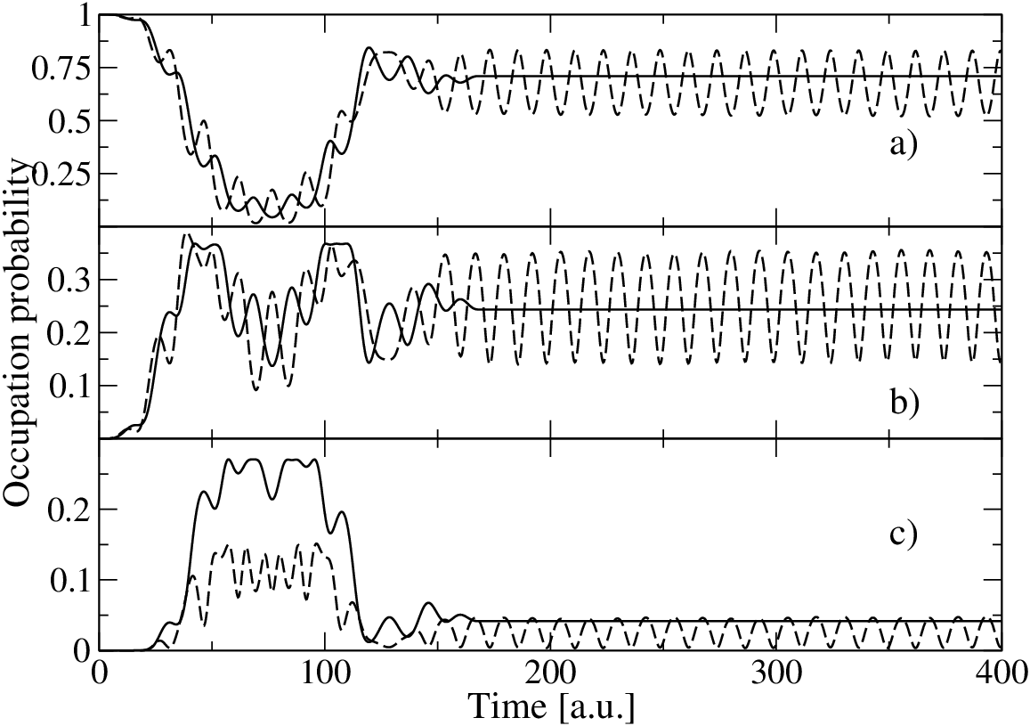The ground state Kohn-Sham equation generates a set of excited virtual Kohn-Sham orbitals $|n\rangle$. Figure 1 shows a comparison of exact occupation probabilities and those obtained from the approximate S-matrix (eq. (7)) by projecting $\Psi^{TDDFT}(t)=\Phi(x_{1},t)\Phi(x_{2},t)$ onto Kohn-Sham Slater determinants. Shown are the occupation of the ground state (figure a, projection onto the Kohn-Sham determinant $|0,0\rangle$), the first excited state (figure b, projection onto $|0,1\rangle$) and the second excited state (figure c, projection onto $0,2\rangle$). The second excited state $|N_{cm}=2,n_{rel}=0\rangle$ involves a configuration mixture of at least two Kohn-Sham Slater determinants to be well represented (configurations $|0,2\rangle$ and $|1,1\rangle$). Neither the projection onto a single Kohn-Sham configuration state $|0,2\rangle$ (figure 1c) nor the projection onto the exact excited state (not shown) yields satisfactory transition probabilities. After the switch-off of the laser, the density undergoes oscillations resulting in time-dependent Hartree and exchange correlation potentials which give rise to oscillations in the occupation probabilities. These are the signatures of the ”spurious cross-channel correlations” well-known from TDHF griffin; alhassid. For the present system, exact excited final states can be easily calculated. We have checked that cross-channel correlations persist when we project onto exact exit-channel states rather than Kohn-Sham determinants. Moreover, we also tested channel states obtained from a TDDFT linear-response equation. In this equation the exchange-correlation kernel of TDDFT was approximated by the exchange-only time-dependent optimized effective potential ullrich; lr and the exact Kohn-Sham orbitals obtained by the exact ground state exchange-correlation potential have been used. The obtained excited-state wavefunctions, however, do not significantly differ from the single Kohn-Sham Slater determinants although the excitation energies are considerably improved compared to the Kohn-Sham energy differences. With presently available approximations to the exchange-correlation kernel, TDDFT linear-response theory does not provide improved excited-state wavefunctions. We thus conclude that the projection amplitude of eq. (7) is not well-suited to determine an approximate S-matrix within TDDFT.
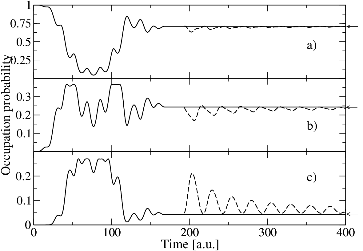
To test the newly proposed read-out functional which depends only on the density, we use the exact time-dependent density $n(x,t)$. In this way, errors due to the approximate exchange-correlation potential can be ruled out and the quality of the proposed functional for state-to-state transition probabilities can be directly assessed. The sum in eqs. (12), (13) and (14) is truncated after the second excited state. Figure 2 shows a comparison of transition probabilities obtained by projecting the wavefunction according to eq. (3) (solid line) and by the new density functional of eq. (14) (dashed line) for the three lowest lying states. In the limit of $t\rightarrow\infty$, i.e. as the averaging interval in eq. (12) increases, the transition probability converges within the numerical accuracy towards the exact result. Numerical errors are due to the truncation of the sum over final states in eq. (14). Note that simply averaging over the cross-channel correlation in eq. (7)(see figure 1) would lead, in general, to incorrect results. Similar good agreement can be found for other initial states and other systems nina.
In conclusion, we have investigated two different methods to extract state-to-state transition amplitudes from TDDFT calculations. In the first method, the correlated many-body wavefunction is approximated by a Slater determinant of the time-dependent Kohn-Sham orbitals. This approximate wave-function is projected onto appropriate final states (exact states or Kohn-Sham configuration states). The resulting state-to-state transition probabilities suffer oscillations after the switch-off of the external perturbation. The second read-out functional to calculate state-to-state transition probabilities directly involves the time-dependent densities and represents thus a well-suited density functional within the framework of TDDFT. The problem of cross-channel correlations can be avoided and well-defined transition probabilities can be determined in the asymptotic limit $t\rightarrow\infty$. First results obtained by evaluating the read-out functional with densities resulting from the exact solution of a one-dimensional two-electron Schrödinger equation are very promising. The application of the read-out functional to double excitation of helium are currently being investigated. Work supported by FWF-SFB 016.

References

- (1) E. Runge, E.K.U. Gross, Phys. Rev. Lett. 52, 997 (1984).
- (2) P. Hohenberg and W. Kohn, Phys. Rev. 136, B864 (1964)
- (3) M.E. Casida, in Recent developments and applications of modern density functional theory, edited by J.M. Seminaro (Elsevier, Amsterdam, 1996)p. 391
- (4) M. Petersilka, E.K.U. Gross, K. Burke, Int. J. Quant. Chem. 80, 534 (2000).
- (5) D.G. Lappas, R. van Leeuwen, J. Phys. B: At. Mol. Opt. Phys. 31, L249 (1998)
- (6) M. Petersilka, E.K.U. Gross, Laser Physics 9, 105 (1999).
- (7) J. Werschnik, E.K.U. Gross, J. Chem. Phys. 123, 62206 (2005).
- (8) P. Bonche, S. Koonin, J.W. Negele, Phys. Rev. C 13, 1226 (1976).
- (9) J.J. Griffin, P.C. Lichtner, M. Dworzecka, Phys. Rev. C 21, 1351 (1980).
- (10) Y. Alhassid, S.E. Koonin, Phys. Rev. C 23, 1590 (1981).
- (11) J.W. Negele, Rev. Mod. Phys. 54, 913 (1982)
- (12) A. Görling, M. Levy, Phys. Rev. B 47, 13105 (1993).
- (13) A. Görling, M. Levy, Phys. Rev. A 50, 196 (1994).
- (14) M. H. Beck, A. Jäckle, G. A. Worth and H.-D. Meyer, Physics Reports 324, 1 (2000).
- (15) J. Zanghellini, M. Kitzler, T. Brabec, A. Scrinzi, J. Phys. B: At. Mol. Opt. Phys. 37, 763 (2004).
- (16) Angel Rubio, private communications
- (17) M. Taut, Phys. Rev. A 48, 3561 (1993).
- (18) P.M. Laufer, J.B. Krieger, Phys. Rev. A 33, 1480 (1986)
- (19) R. Grobe, J.H. Eberly, Phys.Rev.A 48, 4664 (1993).
- (20) J.F. Dobson, Phys. Rev. Lett. 73, 2244 (1994).
- (21) G. Vignale, Phys. Rev. Lett. 74, 3233 (1995).
- (22) I. D’Amico, G. Vignale, Phys. Rev. B 59, 7876 (1999).
- (23) M. Lein, S. Kümmel, Phys. Rev. Lett. 94, 143003 (2005)
- (24) J. P. Perdew, A. Zunger, Phys. Rev. B 23, 5048 (1982).
- (25) C.A. Ullrich, U.J. Gossmann, E.K.U. Gross, Phys. Rev. Lett. 74, 872 (1995).
- (26) N.Rohringer, S.Peter, J.Burgdörfer to be published