Inelastic scattering of light by a cold trapped atom:
Effects of the quantum center-of-mass motion

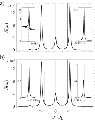
In this section we report and discuss the theoretical results, whose derivation is reported in Sec. III. Figure 2 displays the spectra of the light scattered by the dipole transition of an ion which is sideband-cooled Stenholm86; Eschner03. The spectra have been evaluated for different parameter regimes. Figures 2(a) and (b) correspond to the spectrum at two different detection angles in the situation in which the linewidth of the dipole transition $\gamma=\nu/3$. Here, the mechanical effects of atom-photon interaction are clearly evident in the sidebands of the elastic peak, the two narrow signals at frequency $\omega_{L}\pm\nu$. Their width scales with the recoil frequency and corresponds with the cooling rate Lindberg86; Cirac93; Bienert04. These resonances are magnified in the inset, where one can see that their centers are slightly shifted from the values $\omega_{L}\pm\nu$. This shift is due to the mechanical coupling Cirac93; Bienert04. The corresponding curves are a superposition of Lorentz and Fano-like profiles, whereby one functional dependence can dominate over the other depending on the angle of observation. The asymmetry of these peaks is due to interference effects, which originate from the quantum nature of the ion center-of-mass motion, and whose magnitude depends on the detection angle Cirac93. Manifestations of the mechanical effects in the inelastic spectrum are small but yet visible in Fig. 2(b), causing the appearance of an additional resonance on the left part of the curve (at $\omega=\omega_{L}-2.4\nu$) and a broadening of the central inelastic peak. The width of the sidebands of the inelastic peaks is substantially the same as the one of the corresponding inelastic peak at zero order in the motion. Their height scales with the recoil frequency, and, like the sidebands of the elastic peak, it is a non-trivial function of the average phononic excitation $\langle n\rangle$ and of the angle of detection. Their functional form is reported in Sec. III.2.

Figures 2(c) and (d) display the spectra of fluorescence when the linewidth $\gamma=\nu/10$. Here, the mechanical effects can be clearly identified in the inelastic spectrum, displaced by about $\pm\nu$ from the corresponding signal of the Mollow triplet. The sidebands of the central inelastic peak are centered at the same frequency as the Stokes and anti-Stokes signals, and give rise to a small broadening at their basis.

We remark that the height of the mechanical sidebands – for elastic and inelastic scattering – critically depends on the detection angle, as it is visible in the figures. Also for the inelastic spectrum this effect is caused by interference of the underlying atomic processes contributing to each spectral signature and depending on the direction of photon absorption and emission. Thus, the behavior also depends on whether the drive is a traveling wave, as in Fig. 2, or a standing wave. Figure 3 shows the spectrum of an ion where the trap center is in a point of the standing wave (away from the nodes and anti-nodes), for $\gamma=\nu/10$ and at two different detection angles. Here, one can observe the dependence of the sidebands of the elastic and inelastic part on the detection angle. Figure 4 displays the spectra of resonance fluorescence at various points of the standing wave. For $\varphi=\pi/4$, Fig. 4(a), the spectrum is governed by the outstanding sidebands of the elastic peak, overtopping the Mollow triplet. At $\varphi=3\pi/8$, Fig. 4(b), the trap is closer to the node of the standing wave. Here, the resonances of the Mollow triplet get closer. In this case, the height of the sidebands of the elastic peak decrease and the sidebands of inelastically scattered light are visible. A peculiar case is found when the atom is placed at the node, Fig. 4(c) at $\varphi=\pi/2$. Here, the only spectral signals are the motional sidebands. These sidebands are now perfect Lorentzian curves of identical shape independent of the detector position, as already pointed out in Cirac93. What is novel is that all other contributions of the spectrum, elastic and inelastic, disappear due to the vanishing of the driving field at the center of the trap. In particular, even the motional sidebands of the inelastic spectrum disappear. The appearance of the sidebands of the elastic peak is due to the effects of the gradient of the field intensity over the atomic wavepacket at the node. The suppression of inelastic scattering processes, included the ones that change the motional excitation, can be understood by considering that there are no quantum fluctuations of the atomic dipole at the node of a standing wave.

These behaviors are discussed in detail in the following theoretical treatment. It should be remarked that the sidebands of the inelastic component become visible when the transition, at zero order in the mechanical effects, is driven at saturation. Below saturation the mechanical effects in the inelastic spectrum manifest in small sidebands of the Lorentz curve centered at the laser frequency. These sidebands are at the same frequencies as the ones of the Stokes and anti-Stokes components of the elastic peak, and are covered by these signals.

We introduce now the basic elements determining the dynamics of the atom. The coupling with radiation is assumed to be in the Lamb-Dicke regime. This regime is characterized by the small value of the Lamb-Dicke parameter

which scales the coupling between internal and external atomic degrees of freedom due to photon scattering. We identify $\eta$ as the parameter of the perturbative expansion. According to this expansion, at second order the spectrum in Eq. (4) is decomposed into the terms

where the subscripts label the corresponding order in the Lamb-Dicke expansion. In order to evaluate $S_{j}(\omega)$, we consider the operators ${\cal L}$ and $D$ at second order in the expansion in $\eta$. The dipole $D(x)=D_{0}+D_{1}+D_{2}+{\rm O}(\eta^{2})$, where the individual terms have the form

with $\sigma=|g\rangle\langle e|$. The Liouville operator is decomposed into the terms ${\cal L}={\cal L}_{0}+{\cal L}_{1}+{\cal L}_{2}$, which we now introduce in detail. At zero order internal and external degrees of freedom are decoupled, namely

where ${\cal L}_{\rm E}$ and ${\cal L}_{\rm I}$ act on the external and internal degrees of freedom, respectively. Here,

with

where $a$ and $a^{\dagger}$ are the annihilation, creation operators of a quantum of energy $\hbar\nu$, respectively. We denote with $|n\rangle$ the eigenvectors of $H_{\rm mec}$, fulfilling $H_{\rm mec}|n\rangle=\hbar\nu(n+1/2)|n\rangle$ with $n=0,1,2,\ldots$ The term ${\cal L}_{\rm I}$ acts on the internal degrees of freedom and it is defined as

where $H_{0}=\hbar\delta|g\rangle\langle g|$, with $\delta=\omega_{L}-\omega_{0}$, and

are the interaction with radiation at zero order in the mechanical effects. Here, we have denoted by $\Omega\zeta(\varphi)$ the laser Rabi frequency, whereby $\zeta(\varphi)$ is a dimensionless function of the angle $\varphi$, which is $\zeta(\varphi)=\exp({\rm i}\varphi)|_{\varphi=0}$ for a traveling wave drive, and is given by $\zeta(\varphi)=\cos\varphi$ for a standing wave drive.

The first and second order Liouvillian give rise to the mechanical coupling between internal and external degrees of freedom,

where

Here, $\theta$ is the angle between the laser and the trap axis, $\beta$ is a constant, which gives the average recoil due to spontaneous emission of a photon, and $\zeta^{\prime}(\varphi)$, $\zeta^{\prime\prime}(\varphi)$ are the first and second derivative of $\zeta(\varphi)$ with respect to $\varphi$.

The spectral decomposition of the Liouville operator is obtained using the eigenvalues and eigenelements of operator ${\cal L}_{0}$, of which we evaluate the corrections at second order in $\eta$. We denote the eigenvalues and eigenelements of ${\cal L}_{0}$ by $\lambda_{0}$ and $\varrho_{0}^{\lambda}$, $\check{\varrho}_{0}^{\lambda}$, respectively. Since internal and external degrees of freedom are decoupled at zero order in $\eta$, the eigenvalues of ${\cal L}_{0}$ are $\lambda_{0}=\lambda_{\rm I}+\lambda_{\rm E}$, and the eigenelements

where ${\cal L}_{\rm I}\rho^{\lambda_{\rm I}}=\lambda_{\rm I}\rho^{\lambda_{\rm I}}$ and ${\cal L}_{\rm E}\mu^{\lambda_{\rm E}}=\lambda_{\rm E}\mu^{\lambda_{\rm E}}$. Correspondingly, the projector into the subspace at the eigenvalue $\lambda_{0}$ is

whereby their action on the operator $X$ is defined as

and ${\rm Tr}_{\rm I}$ (${\rm Tr}_{\rm E}$) denotes the trace over the internal (external) degrees of freedom.

The spectrum of ${\cal L}_{\rm I}$ characterizes the dynamics of the two-level transition and the spectral properties of the radiation emitted by the bare atom Jakob03. The eigenvalues of ${\cal L}_{\rm E}$ take on the values $\lambda_{\rm E}={i}\ell\nu$, with $\ell=0,\pm 1,\pm 2,\ldots$ Each eigenspace at $\lambda_{\rm E}$ is infinitely degenerate, and the corresponding left and right eigenelements are, for instance, $\check{\mu}_{n}^{\ell}=|n+\ell\rangle\langle n|$, $\mu^{\ell}_{n}=|n\rangle\langle n+\ell|$. These eigenelements constitute a complete and orthonormal basis over the eigenspace at this eigenvalue. In particular, the projector over the eigenspace at $\lambda_{\rm E}={i}\ell\nu$ is defined on an operator $X$ as

where ${\rm Tr}_{\rm E}$ denotes the trace over the external degrees of freedom.

At higher orders in the expansion in $\eta$, internal and external degrees of freedom are coupled, and the degeneracy of the subspaces at eigenvalue $\lambda_{\rm E}$ is lifted Lindberg84; Stenholm86. The perturbative corrections to the eigenvalues $\lambda_{0}$, to the eigenelements $\rho^{\lambda}_{0}$, $\check{\rho}^{\lambda}_{0}$, and to the projectors ${\cal P}^{\lambda}_{0}$ are found by solving iteratively the secular equations at the same order in the perturbative expansion, and are given by

where ${\cal P}^{\lambda}_{0}$ is the zero-order projector onto the subspace at eigenvalue $\lambda$, ${\cal P}^{\lambda}_{0}=\varrho_{0}^{\lambda}\otimes\check{\varrho}_{0}^{\lambda}$. Using (17) we obtain

Analogously, one finds the perturbative corrections to the left eigenelements $\check{\varrho}^{\lambda}_{0}$. This in turn allows one to evaluate the perturbative corrections to the projectors ${\cal P}^{\lambda}_{0}$, which are immediately found by using the explicit form of $\check{\varrho}^{\lambda}_{j}$, $\varrho^{\lambda}_{j}$ into the relations

The equations for the corrections $\lambda_{1}$, $\lambda_{2}$ to $\lambda_{0}$ are

where we have used relation ${\cal P}^{\lambda}_{0}{\cal L}_{1}{\cal P}^{\lambda}_{0}=0$ in Eq. (21).

A relevant eigenelement of this spectral decomposition is the one at $\lambda_{0}=0$, namely the steady-state density matrix. At zero order this is given by $\varrho_{0}^{\lambda=0}=\rho_{0}\mu$, where $\mu$ is the density matrix for the external degrees of freedom in the final stage of the laser-cooling dynamics and has the form

and

is the average phonon number at steady state. Correspondingly, $\check{\varrho}_{0}^{\lambda=0}=\mathds{1}_{\rm I}\mathds{1}_{\rm E}$, where $\mathds{1}_{j}$ is the identity for the Hilbert space of the internal ($j={\rm I}$) and the external ($j={\rm E}$) degrees of freedom.

We now proceed in evaluating the spectrum of resonance fluorescence using the terms introduced in the previous section. At zero order in the mechanical effects, the spectrum is

where $G(\lambda)={\rm Tr}\{D_{0}^{\dagger}{\cal P}^{\lambda}_{0}D_{0}\rho_{0}\}$, which corresponds to the spectrum of the bare atomic dipole. It thus exhibit peaks which are located at frequencies equal to the real part of the eigenvalues $\lambda_{\rm I}$, whose width is determined by the imaginary part of $\lambda_{\rm I}$. Note that ${\rm Tr}\{D_{0}^{\dagger}{\cal P}^{\lambda}_{0}D_{0}\rho_{0}\}={\rm Tr}\{\sigma^{\dagger}\rho_{0}^{\lambda_{\rm I}}\}{\rm Tr}\{\check{\rho}_{0}^{\lambda_{\rm I}}\sigma\rho_{0}\}.$ For later convenience, we introduce the scalar functions

such that with this notation $G(\lambda)=g(\lambda_{\rm I}){\check{g}}(\lambda_{\rm I})$.

The term $S_{1}(\omega)=0$, since the motional steady state $\mu$, Eq. (23), is a thermal state, and thus diagonal in the vibrational number basis Bienert04.

The features due to the mechanical effects thus manifest at second order in the Lamb-Dicke expansion, and the corresponding term has the form

where

The function $F(\lambda)$ can be decomposed into three contributions, namely

This decomposition allows one to identify the effects of the quantum motion on the features of the spectrum. The term $F_{0}(\lambda_{\rm I})$ is a second-order correction to the features of the zero order spectrum, $S_{0}(\omega)$. Namely, it gives rise to small corrections to the curves of the zero-oder spectrum, however it does not affect relevantly its general form. The terms $F_{\pm}(\lambda_{\rm I})$, on the other hand, give rise to novel peaks centered at the frequencies ${\rm Im}\{\lambda_{\rm I}\}\pm\nu$, which can be identified with the sidebands of the peaks appearing in $S_{0}(\omega)$. These terms have the form

and

where we have used $\eta=kx_{0}$ with $x_{0}=\sqrt{\hbar/2m\nu}$ and we have introduced the functions

The basic steps that lead to Eqs. (III.2)-(34) are reported in App. A. The results are plotted and discussed for some parameter regimes in Sec. II.

We now discuss some general properties of the equations for two cases: When the laser, driving the dipole and cooling the motion, is a traveling wave and when it is a standing wave.

Traveling wave drive. The case when the driving laser is a traveling wave is found by setting $\zeta^{\prime}(\varphi)=i$ at $\varphi=0$ in Eq. (13). We evaluate the terms Eqs. (31) - (34) using the zero-order eigenelements $\rho^{\lambda}_{0}$ and $\check{\rho}^{\lambda}_{0}$ determined by the eigenvalue equations ${\mathcal{L}}_{0}\rho_{\rm I}^{\lambda}=\lambda_{0}\rho_{\rm I}^{\lambda}$ and $\check{\rho}^{\lambda}_{\rm I}{\mathcal{L}}_{0}=\lambda_{0}\check{\rho}^{\lambda}_{\rm I}$, as in Jakob03. The eigenvalue $\lambda_{\rm I}=0$ gives the contribution of the elastic peak. As we focus on the case of a dipole driven at saturation, the three other – nonvanishing – eigenvalues of the zero-order spectrum determine the position and the widths of the Mollow peaks.

We characterize the higher-order contributions to the spectrum by their corresponding eigenvalues at zero order and analyze the single terms composing $S_{2}(\omega)$, Eq. (26). As $S_{0}(\omega)$ never vanishes for traveling wave drives, the term $F_{0}$ gives rise to small corrections to the elastic peak (component at $\lambda_{\rm I}=0$) and to the Mollow spectrum (components at $\lambda_{\rm I}\neq 0$). The terms $F_{\pm}(\lambda)$ correspond to novel peaks which add to the ones of the zero-order spectrum. At $\lambda_{\rm I}=0$ these terms give rise to the motional sidebands of the elastic peak, centered about $\lambda_{\rm E}=\pm i\nu$. In this case the terms Eqs. (31) - (34) have to be evaluated for $\check{\rho}_{0}^{\lambda_{\rm I}}=\mathds{1}_{\rm I}$ and $\rho_{0}^{\lambda_{\rm I}}=\rho_{0}$. By applying the cyclic properties of the trace one finds that $u(0,\lambda_{\rm E})=0$ and that $r_{\ast}(0,\lambda_{\rm E})=r(0,\lambda_{\rm E})^{\ast}$. Since $\lambda_{\rm I}=0$, the width and shape of these curves is critically determined by the second order correction $\lambda_{2}$ to the eigenvalue. The explicit evaluation can be found in Lindberg84; Bienert04. The result we find is in agreement with the one reported in Cirac93.

The mechanical effects on the inelastic part of the spectrum manifest themselves in the components at $\lambda_{\rm I}\neq 0$. They give rise to small shifts of the center-frequency ${\rm Im}\{\lambda_{\rm I}\}$ and of the linewidth ${\rm Re}\{\lambda_{\rm I}\}$, and to novel peaks which are centered at the frequencies ${\rm Im}\lambda_{\rm I}\pm\nu$, and which we discuss in the following. These peaks are the sidebands of the corresponding zero-order curves in the Mollow spectrum. Their width is the width of the corresponding zero-oder Mollow peak, namely ${\rm Re}\{\lambda_{\rm I}\}$. The intensity of the particular signals is proportional to $F_{\pm}(\lambda_{\rm I})$, where generally all the terms (31) - (34), $g(\lambda_{\rm I})$ and $\check{g}(\lambda_{\rm I})$ contribute. Their shape is in general a superposition of Lorentz (real part of $F_{\pm}(\lambda_{\rm I})$) and Fano-like (imaginary part of $F_{\pm}(\lambda_{\rm I})$) curves. Note that in the plots shown in Sec. II, the real part of $F_{\pm}(\lambda_{\rm I})$ dominates for the visible peaks and thus these sidebands appear as Lorentz curves in the spectrum. Their visibility, however, depends on the detection angle. Indeed, also for these terms there are interference effects that give rise to an asymmetry between the right and the left sideband of a given inelastic peak. Note that the sidebands of the central inelastic peak are located at the same frequencies of the Stokes and anti-Stokes sidebands. These terms do not vanish, but are usually hidden by the Stokes and anti-Stokes contributions. Spectra for different parameter regimes are shown in Fig. 2.

Standing wave drive. The case when the driving laser is a standing wave is found by setting $\zeta(\varphi)=\cos\varphi$ in $V_{0}$ and $\zeta^{\prime}(\varphi)=-\sin\varphi$ in Eq. (13). The general characteristic of the terms composing the spectrum is basically the same as for a traveling wave, the difference arises mainly in the dependence of the curves on the scattering angle. The analytical form of the two sidebands, which we obtain by evaluating explicitly $F_{\pm}(0)$ and the linewidth $\lambda_{2}$ of the resonances, is in agreement with the formulas reported in Cirac93. A peculiar behavior is found if the atom is placed at the node of the standing wave, $\zeta(\varphi)=0$, which we discuss in the following. Indeed, in the node of a standing wave the electromagnetic field vanishes at zero order in the Lamb-Dicke expansion. Hence, the dipole is excited by processes at higher order in the Lamb-Dicke parameter $\eta$. In other words, in this regime the spectrum of resonance fluorescence is only due to the gradient of the electromagnetic field over the finite size of the ion wave packet, and thus originates from mechanical effects of atom-photon interaction. In the formulas the terms $V_{0}=V_{2}=0$ and the steady-state density matrix $\rho_{0}=|g\rangle\langle g|\mu$. Details over the eigenelements and eigenvalues of ${\cal L}_{\rm I}$ are reported in App. B. In this case $D_{0}\rho_{0}=0$ and consequently the term $u(\lambda)=0$, see Eqs. (). For the same reason the second term on the RHS of $t(\lambda)$ vanishes, see Eq. (34). Also the first term on the RHS of $t(\lambda)$ vanishes, as one can verify by taking the explicit form of $V_{1}$, Eq. (13), and of the eigenelements. Hence $t(\lambda)=0$. Moreover, in App. B we show that $F_{0}(\lambda)=0$. The only terms which do not vanish are $r(0,\lambda_{\rm E})$ and $r_{*}(0,\lambda_{\rm E})$ in $F_{\pm}(\lambda)$, Eqs. (31)-(32). Therefore, the spectrum is at second order in the Lamb-Dicke expansion, and the only non-vanishing contributions are the Stokes and anti-Stokes sidebands of the elastic peak. Spectra evaluated for different parameters are shown in Figs. 3 and 4.

References

- (1) For a recent review, see D. Leibfried, R. Blatt, C. Monroe, and references therein. D. Wineland, Rev. Mod. Phys. 75, 281 (2003).
- (2) P.S. Jessen, C. Gerz, P.D. Lett, W.D. Phillips, S.L. Rolston, R.J.C. Spreeuw, and C.I. Westbrook, Phys. Rev. Lett. 69, 49 (1992); M. Gatzke, G. Birkl, P.S. Jessen, A. Kastberg, S.L. Rolston, and W.D. Phillips, Phys. Rev. A 55, R3987 (1997).
- (3) J.T. Höffges, H.W. Baldauf, T. Eichler, S.R. Helmfrid, H. Walther, Opt. Commun. 133, 170 (1997); J.T. Höffges, H.W. Baldauf, W. Lange, H. Walther, J. Mod. Opt. 44, 1999 (1997).
- (4) Ch. Raab, J. Eschner, J. Bolle, H. Oberst, F. Schmidt-Kaler, R. Blatt, Phys. Rev. Lett. 85, 538 (2000).
- (5) V. Bühner and Chr. Tamm, Phys. Rev. A 61, 061801(R) (2000).
- (6) M.A. Wilson, P. Bushev, J. Eschner, F. Schmidt-Kaler, C. Becher, R. Blatt, and U. Dorner, Phys. Rev. Lett. 91, 213602 (2003).
- (7) P. Bushev, A. Wilson, J. Eschner, C. Raab, F. Schmidt-Kaler, C. Becher, and R. Blatt Phys. Rev. Lett. 92, 223602 (2004).
- (8) P. Bushev, D. Rotter, A. Wilson, F. Dubin, Ch. Becher, J. Eschner, R. Blatt, V. Steixner, P. Rabl, P. Zoller, quant-ph/0509125.
- (9) M. Lindberg, Phys. Rev. A 34, 3178 (1986).
- (10) J.I. Cirac, R. Blatt, A.S. Parkins, and P. Zoller, Phys. Rev. A 48, 2169 (1993).
- (11) G.C. Hegerfeldt and M.B. Plenio, Phys. Rev. A 52, 3333 (1995).
- (12) M. Bienert, W. Merkel, and G. Morigi, Phys. Rev. A. 69, 013405 (2004), see also M. Bienert Manifestations of Mechanical Effects of Light in Atom Optics, PhD-Thesis, University of Ulm, 2004 (Mensch & Buch Verlag, Berlin 2004, ISBN 3-89820-791-9).
- (13) Th. Becker, J. v. Zanthier, A. Yu. Nevsky, Ch. Schwedes, M. N. Skvortsov, H. Walther, and E. Peik, Phys. Rev. A 63, 051802(R) (2001); E. Peik, J. Abel, Th. Becker, J. von Zanthier, and H. Walther, Phys. Rev. A 60, 439 (1999).
- (14) S.M. Barnett and S. Stenholm, J. Mod. Opt. 47, 2869 (2000); see also S.M. Barnett and S. Stenholm, Phys. Rev. A 64, 033808 (2001), and references therein.
- (15) H.J. Briegel and B.-G. Englert, Phys. Rev. A 47, 3311 (1993); For a review, see B.-G. Englert and G. Morigi, in Coherent Evolution in Noisy Environments, Lecture Notes in Physics 611, p. 55, ed. by A. Buchleitner, K. Hornberger (Springer Verlag, Berlin-Heidelberg-New York 2002), and references therein.
- (16) M. Jakob and S. Stenholm, Phys. Rev. A 67, 032111 (2003)
- (17) B.R. Mollow, Phys. Rev. 188, 1969 (1969).
- (18) C. Cohen-Tannoudji, J. Dupont-Roc, G. Grynberg, Atom-Photon Interactions, J. Wiley and Sons ed. (Toronto, 1992).
- (19) S. Stenholm, Rev. Mod. Phys. 58, 699 (1986).
- (20) J. Eschner, G. Morigi, F. Schmidt-Kaler, and R. Blatt, J. Opt. Soc. Am. B 20, 1003 (2003).
- (21) H.J. Carmichael, An Open Systems Approach to Quantum Optics, Springer-Verlag (Berlin, Heidelberg, New York, 1993)
- (22) J. Javanainen, M. Lindberg and S. Stenholm, J. Opt. Soc. Am. B 1, 111 (1984); M. Lindberg and S. Stenholm, J. Phys. B 17, 3375 (1985).