Semantics and Simulation
of Communication in
Quantum Programming
Diploma Thesis
Wolfgang Mauerer1
Quantum Information Theory Group
Institute for Theoretical Physics I and
Max Planck Research Group for Optics,
Information and Photonics
University Erlangen-Nuremberg, May 2005
Abstract We present the quantum programming language cQPL which is an extended version of QPL [Sel04b]. It is capable of quantum communication and it can be used to formulate all possible quantum algorithms. Additionally, it possesses a denotational semantics based on a partial order of superoperators and uses fixed points on a generalised Hilbert space to formalise (in addition to all standard features expected from a quantum programming language) the exchange of classical and quantum data between an arbitrary number of participants. Additionally, we present the implementation of a cQPL compiler which generates code for a quantum simulator. PACS numbers: 03.67.-a, 03.67.Hk, 03.67.Lx, 89.20.Ff Revision 1.1 (15. September 2005)
1 eMail: wmauerer@optik.uni-erlangen.de
Chapter 1 Introduction
Dich sah ich, und die milde Freude
Floß von dem süßen Blick auf mich;
Ganz war mein Herz an deiner Seite
Und jeder Atemzug für dich.Johann Wolfgang von Goethe, Willkommen und Abschied Although there
is no formal proof that quantum computers offer greater computational
power than classical ones, there are a few quantum computer algorithms
which provide efficient solutions for problems which are up to now
believed to be classically NP-hard, i.e., they cannot be solved in
polynomial time. One of these problems – computing discrete
logarithms – is the cornerstone of basically every modern classical
cryptographic algorithm, so the increased interest in quantum
computing is obvious, both from a fundamental and a practical point of
view.
How can quantum algorithms be described in an efficient, readable and precise manner? Usually, this is done with quantum circuits which are combined into a quantum network, but especially for larger programs, this is a very cumbersome and error-prone method. Much research has been performed on the construction, implementation and conception of classical programming languages; therefore, a great amount of alternatives are available. The situation is totally different in quantum computing: Only a handful of languages have been proposed so far [AG04, BSC01, Öme98, SP00, Sel04b, vT04], and only two working implementations based on quantum computer simulators are available [Öme98, BSC01] (recently, a third, but still rough implementation was presented in [AG05]). Both are based on imperative/object oriented languages (C, Pascal, C++, …), with quantum features as extensions, whereas QPL [Sel04b] models a basically functional language.11 1 We need to note, though, that the term functional should not be overestimated in this context. Important features like higher order functions, which are considered to be key elements of classical functional languages, are missing in QPL. The most interesting part of the language from a physicist’s point of view is the ability to guarantee freedom against runtime errors already at compile time, no matter how this goal is achieved.
In this work, we present an extension of QPL with abilities to cover quantum communication, i.e., the transmission of quantum mechanical states and exploitation of their highly non-classical properties like superpositions and entanglement. To distinguish our approach from QPL, we call it cQPL for communication capable QPL. In contrast to quantum computers of which only some very elementary parts have been experimentally realised until now, implementations of quantum communication are not only available in several laboratories around the world, but can even be obtained commercially.
To provide some orientation where our approach can be located in contrast to work done by other contributors to the field, Table 1.1 presents a comparison of quantum programming languages and their features.
| QCL | Q Language | qGCL | QML | QPL | cQPL | |
|---|---|---|---|---|---|---|
| Reference | [Öme98] | [BSC01] | [SP00] | [AG04] | [Sel04b] | |
| New language | ✗ | ✗ | ✓ | ✓ | ✓ | ✓ |
| Respects physics22 2 Respecting physics is meant in the sense that it is not possible to syntactically specify programs which would create unphysical situations; of course, such a state will force the simulation to abort with an error and needs thus to be avoided if possible. | ✗ | ✗ | ✗ | ✓ | ✓ | ✓ |
| Implemented | ✓ | ✓ | ✗ | ✓33 3 A partially finished implementation was available at the time of writing. | ✓44 4 If we consider our cQPL compiler to be a QPL compiler as well. | ✓ |
| Formal semantics | ✗ | ✗ | ✓ | ✓ | ✓ | ✓ |
| Communication | ✗ | ✗ | ✓ | ✗ | ✗ | ✓ |
| Universal | ✓ | ✓ | ✓ | ✓ | ✓ | ✓ |
In a nutshell, the contribution of our work to the field of quantum programming languages is twofold:
- ❏
We provide a compiler which can serve as a testbed for new ideas in quantum programming, to teach concepts of quantum algorithms or act as an aid to the intuition of users who want to experiment (in the sense of goal oriented playing, not laboratory) with quantum protocols.
- ❏
We present an alternate approach to the compositional semantics of QPL and provide the possibility to include and formalise quantum communication as part of the language. This is a necessary step towards the formalisation of open-world programs, but may also prove itself useful in fields like quantum process calculi, automated protocol analysis or similar – cf. Chapter 6 for further prospects.
The layout of this thesis is as follows: In Chapters 2 and 3, we provide an overview about quantum programming, present the language cQPL and describe the compiler and its implementation. Chapter 4 presents the mathematical tools and requisites necessary for a denotational semantics of cQPL, and Chapter 5 develops the semantical description. Chapter 6 finally provides some short remarks on possible further directions that may be pursued based on the results of this work. All chapters are interlaced with short introductions to topics, tools and techniques which are uncommon in physics, but necessary for our work; Appendices A and B provide a list of symbols and a glossary, respectively. The formal syntax is presented in Appendix C. To aid the reader in staying on track, we have provided short summaries in grey boxes at some points along the way.
Since the topic dealt with does not only contain problems of physical nature, but also touches the fields of computer science and mathematics, we have tried to make the text as self-contained as possible for readers with any of these backgrounds.55 5 In this context, it is interesting to note that of all entries in the bibliography are of physical nature and can be counted to computer science; the remaining belong to mathematics or are of general interest. Obviously it was not possible to present everything in as much detail as required without repeating the introductory textbooks, but numerous references to the literature are provided which hopefully alleviates any arising problems.
Chapter 2 Quantum programming with QPL and cQPL
When someone says, “I want a programming language in which I need only say what I wish done,” give him a lollipop. Alan Perlis, Epigrams on Programming This chapter presents an overview about classical and quantum computers, the underlying models of computation and some principal remarks on quantum programming languages. Afterwards, a short introduction to QPL and cQPL is given. Note that this chapter is intentionally kept as terse as possible to allow a more detailed coverage of other topics dealt with in this thesis. Therefore, no attempt is made to to provide special rigour in this chapter.
2.1 Programming and quantum physics
2.1.1 Computability
Classical computers can be described by several models which are apt for different purposes (for a more detailed description, cf., e.g., [AB02, Sch01]):
- ❏
Turing machines
- ❏
General recursive functions
- ❏
Register machines
- ❏
Lambda calculus
- ❏
Logical gates
- ❏
Universal programming languages
They can all be brought to a common denominator by showing that they are able to compute respectively solve the same class of problems. They are computationally equivalent because one model can be used to efficiently simulate any other model; a Turing machine is normally taken to be the normative instance among them. The fact that a turing machine can compute everything which is computable in principle is captured in the Church-Turing thesis which is one of the fundamental axioms of computer science:11 1 To be precise, one would have to note that Church’s thesis states that “a function of positive integers is effectively calculable only if recursive”. This is equivalent to Turing’s thesis, though, and the name Church-Turing thesis is conventionally used in the literature.
Hypothesis 2.1.1 (Church-Turing).
Every function which would naturally be regarded as computable can be computed by a Turing machine.
This definition places computability in a purely abstract setting without regard to the laws of physics. Deutsch [Deu85] realised that if the laws of (quantum) physics are used as basis for computation, an improved version of the Turing machine might lead to greater computational power. This requires an extended version of the Church-Turing thesis as well:
Hypothesis 2.1.2 (Church-Turing-Deutsch).
Every physical process can be simulated by a universal computing device.
Greater computational power is meant in the sense that there are some problems which can be efficiently solved by a universal computing device according to Church-Turing-Deutsch but which cannot be efficiently solved by a Turing machine, e.g., the simluation cost for a universal computing device on a normal turing machine would be at least exponential for the most general case.22 2 Note that there is a very prominent problem which illuminates this field: Factorising integers is possible at polynomial cost on a quantum computer, but the currently best known algorithms require exponential cost on a classical computer. This does not prove, though, that quantum computers are per se more powerful than classical ones because there is, for example, no proof that there is no classical polynomial-time factorisation algorithm.
2.1.2 Characteristics of quantum computers
The basic building block for quantum computers are quantum bits (qbits), i.e., quantum mechanical objects which can be represented by two different basis states, usually denoted by and . This can, e.g., be realised by two-spin systems such as electrons, with the two different polarisations of a photon etc. In contrast to classical machines and models of computation, quantum computing can draw from two additional resources:
- ❏
Superpositions: The state of a quantum bit can be in a superposition with and . If every qbit of a quantum register consisting of elements is brought into a symmetric superposition with , the register contains all numbers from to at the same time. Manipulations of the register thus manipulate all these numbers in one step, whereas classically, the number of required manipulations would grow exponentially with the register size. This feature is conventionally referred to as quantum parallelism.
- ❏
Entanglement: Two parts of a quantum system can be in an entangled state such that manipulations on one part of the system influence the other system although they may be spatially separated.
While superpositions are useful for computational problems, entanglement is suitable for tasks like secret key growing, but is for example also necessary to connect input with output registers for quantum function application.
In general, there are several equivalent models for quantum computers which are abstracted from their physical realisation:
- ❏
Quantum Turing machines
- ❏
Quantum gates
- ❏
Universal quantum programming languages
2.1.3 Static typing, functionality and runtime errors
Selinger proves in [Sel04b] that QPL has the ability to avoid runtime errors by detecting them at compile time (and can thus reject the program) which is not possible in other language proposals presented at the time of writing. He argues that this must be attributed to the static type system of the language. Although the proof for this is solely based on properties of the static type system, the functional style of QPL does have its merits in this respect in our opinion, too: It restricts the language to elements which allow to express universal programs, but do not allow constructions that can produce runtime errors that cannot be detected at compile time.33 3 A static type system is in general not enough to ensure this property: Just think of the many possible ways to generate runtime-errors in C, which is statically typed as well. This is partially caused by the fact that typing in C is weak; nevertheless, even strongly typed languages as, e.g., Java and C# still cannot prevail runtime errors. Thus, static typing alone is not sufficient to avoid all possible runtime errors.
When work on this thesis was started, one of the points we wanted to investigate was if and how principles of functional languages could be advantageous for quantum languages. This did not reach fruition, though, because we could not find a simple way to transfer any advanced functional method like higher-order functions, recursively defined data types etc. to the quantum case.44 4 To our knowledge, no fully satisfying mechanism for any of these problems has been found until now although the topic is addressed in several papers.
From a physical perspective, the absence of runtime-errors is much more interesting than any computer science related question like the type system or functionality. In this thesis, we thus concentrated on preserving the possibilities of static checking provided by QPL as far as possible while enhancing usability of the language and providing means to handle commuication.
2.2 Introduction to QPL and cQPL
This section presents a very short introduction to cQPL; some of the things stated in the following also hold for a (regularised version) of block QPL55 5 The variant of QPL with a textual structure that includes blocks; alternatively, there is a textual variant without blocks and a flow diagram representation. as presented in [Sel04b] which is used as basis for cQPL. Note that cQPL is explicitely meant to be an experimental compiler. Only very modest effort was made to make the compiler easy to use (the error messages provided can, for example, often only be understood if the user is familiar with the inner working of the compiler), and only very few classical operations which are considered standard components of programming languages (e.g., numerical operations like etc.) were implemented to save time since this is purely routine work. Nevertheless, care has been taken to design the compiler for easy extensibility.66 6 For example, integration of the -qbit Fourier gate could be accomplished by adding only lines of code to the compiler and to the runtime library.
2.2.1 Model of computation
Although quantum gates are the most widespread model in the literature on quantum algorithms, the QRAM model suggested by Knill [Kni96] is more apt as basis for quantum programming languages. The model consists of two components: A classical computer for conventional tasks like program flow control, classical calculations etc., and a quantum memory controlled by the classical computer that can not only store quantum states, but also apply any unitary operator and perform measurements. Figure 2.1 visualises the approach.

cQPL is centred on the assumption that the control flow of a program can be described by classical means. Although this is considered to be a loss of generality by some authors (most notably [Öme03]), it does not represent a real restriction because all known quantum algorithms can be expressed in this framework. Data is, of course, quantum mechanical, and can be modified by unitary operators which are equivalently called gates in analogy to the gate model of quantum computation.
2.2.2 Language elements
The following remarks provide an introduction to cQPL for ordinary users; a formal version of the syntax will be presented in Appendix C. The compiler distribution provides some example programs which demonstrate all features.
2.2.2.1 Identifiers and variables
Identifiers for variables can be denoted by strings consisting of the characters A–Z, a–z, _ and 0–9, where no digit must be at the beginning. Allocation of new variables is done with the operator new:
new int loop := 10;
new qbit b1 := 1;
Note that it is mandatory to provide an initial value both for classical and quantum data types. By default, the data types bit, int, float, qbit and qint are available.
Assigning values to classical variables is possible using the operator :=:
loop := loop - 1;
2.2.2.2 Arithmetic and logical expressions
Arithmetic expressions can be given as in most programming languages (e.g., 7+3*x-5). The operators +, -, * and / are available, they are overloaded to work with any classical numerical data type.
Operators resulting in a logical value (true or false)
are <, >, <=, >=, = and
!=; logical negation is
available using !, and predicates can be combined using
& (and) and | (or). Operator priority
is defined as usual in arithmetic and logic; parentheses can be
used to explicitely modify this.
2.2.2.3 Procedures
Procedures can take an arbitrary number of input parameters (including none) which are specified as name:type tuples. Declarations take the following form:
proc test: a:int, b:bit, c:float, d:qbit {
...
}
Procedure calls are achieved with the keyword call:
(eins, zwei, drei) := call test(a0, a1, a2, b1);
Note that the parameters are passed by value so that modifications of the classical variables given to the procedure (in this case a0, a1 and a2) are not visible in the caller’s scope. This means that no matter what test does, these variables have the same values before and after the procedure is called. This is not the case with b1 because it is a quantum variable and cannot be cloned to implement call-by-value; any modifications performed by test on the state ofb1 are visible for the caller after test returns.
The result of a procedure is a tuple containing the values the classical parameters had at the end of procedure execution; the example stores these in the local variables eins, zwei and drei. Note that the result of a procedure call may be ignored as well by the caller, so the following variant is also possible:
call test(a0, a1, a2, b1);
The example program proc_test.qpl which accompanies the compiler further illustrates the described behaviour, so we refer the reader to it.
2.2.2.4 Gates
Gate application is performed using the operator *= as in the following example:
q *= Not;
A small number of elementary gates is built into the language core (remember that additional ones can be added with really little effort as we already mentioned before):
- ❏
H Hadamard transformation on a qbit.
- ❏
Fourier transformation on qbits, i.e., the -fold tensor product of Hadamard transforms.
- ❏
NOT Logical negation on one qbit.
- ❏
CNot Controlled Not on two qbits.
- ❏
Phase Phase shift gate on one qbit; the desired shift is given as parameter.
The dimension of the gate and the destination must match. Variable tuples where identifiers are combined with commas (,) can be used to combine several quantum variables as in the following example:
new qbit test1 := 0;
new qbit test2 := 1;
test1, test2 *= CNot;
test1 *= Phase 0.5;
User-defined gates can be defined by enclosing a list of (complex) numbers in [[ and ]] as in the following example:
test1,test2 *= [[0.5,  0.5,   0.5,  0.5,
                 0.5,  0.5i, -0.5, -0.5i,
                 0.5, -0.5,   0.5, -0.5,
                 0.5, -0.5i, -0.5,  0.5i]];
2.2.2.5 Control flow
If-then-else and While are available for directing the control flow.
new int loop := 10;
while (loop > 5) do {
    print loop;
    loop := loop - 1;
};

if (loop = 3) then {
    print "3";
}
else {
    print "Nicht 3";
}
The meaning of these operations is the same as in classical languages.
2.2.2.6 Other features
Several more features which do not fit into any of the above categories are available:
- ❏
dump takes one or more quantum variable identifiers as argument and provides a dump of the current probability spectrum in the canonical basis :
dump eins, zwei;
To demonstrate the effect of this command, consider the following example:
new qbit a := 0;
new qbit b := 0;
print "State before FT:"; dump a, b;
a, b *= FT(2);
print "State after FT:";  dump a, b;
The program fragment produces the following output when run:
State before FT: 1 |00>
State after FT: 0.25 |00>, 0.25 |01>, 0.25 |10>, 0.25 |11>
Note that there is a fundamental difference between dumping the state of quantum variables and measuring the state and printing the result, as the following example shows:
measure a then { print "a is |0>"; } else { print "a is |1>"; };
print "State of b:";  dump b;
print "State of (a,b):"; dump a,b;
If the fragment above is supplemented by these lines, running the program either yields this
a is |0>
State of b: 0.5 |0>, 0.5 |1>
State of (a,b): 0.5 |00>, 0.5 |01>
or that output (the output of the statements before is omitted):
a is |1>
State of b: 0.5 |0>, 0.5 |1>
State of (a,b): 0.5 |10>, 0.5 |11>
The result of the command dump b never changes, no matter how often the program is run. The result of the measure command, however, will change so that every output appears with probability for a large number of executions.
- ❏
skip does nothing, but can be used to fulfil syntactic requirements if, for example, one branch of an if-then-else-statement is supposed to do nothing:
if (condition) then { skip; } else { ... } - ❏
print prints the value of a variable or an arithmetic expression (e.g., print 5+7; print a;), but can also be used to output text strings enclosed in quotation marks to the console (e.g., print "Hello, world!";).
- ❏
measure measures a quantum variable and returns a classical result. The result is governed by a probability distribution according to the state the quantum variable is in; thus, successive program runs will in general return different results when the function is called. Note that the measurement is always performed in the standard basis for each contributing qbit.
2.2.3 Modelling quantum communication with cQPL
Although quantum communication has already been implemented with several physical schemes at the time of writing, cQPL does not consider any of these solutions. Instead, the model presented in Section 2.2.1 is extended in such a way that the peculiarities of communication can be replaced by reasonable simulation alternatives. In a real physical setting, communication between two parties can be implemented by using whatever kind of quantum channel which allows to transfer quantum states. Since this is not quite easy to implement experimentally (quantum states are very fragile objects), diverse effects like channel loss, decoherence etc. need to be taken into account in a real-world setting. This is accounted for by a channel model which describes these effects mathematically.
2.2.3.1 Quantum channels
Obviously, no spatial transmission of quantum states is performed in the simulation.77 7 It would be possible, for example, to consider networked computers between which simulated quantum states can be transferred. This would add no new physical insights to the problem, but only add technical difficulties, so we did not implement such a scheme. A quantum channel is thus replaced with a label on each qbit present in the simulation which denotes the respective owner. Sending a qbit is thus equivalent to changing the label of it. Note that this definition differs from the definition of a channel which is used in some contributions to the literature, e.g. [Key02]. Here, a channel is seen as something that modifies the state, for example by decoherence, loss or the influence of eavesdroppers, whereas our definition captures the notion of a channel as a means of unambiguous quantum state transfer. Inclusion of eavesdroppers (or any modification of the quantum state) is possible if a quantum channel is replaced by two quantum channels which are connected by a third module (which we E for Eve following the usual convention) which receives quantum states from Alice, performs appropriate modifications and resends the states to Bob. Obviously, Eve can collect multiple qbits that pass the channel and manipulate them collectively to pursue different attack strategies, so this is in no way a restriction to intercept-resend attacks. Figure 2.2 provides a visualisation of the communication model.

2.2.3.2 Modules and communication primitives
Communicating systems are specified in terms of modules which contain the code the participants execute. Every module is identified by a unique label which identifies it among the participants. Note that module definitions must only occur at the top-level; modules must not contain other module definitions. Two parties which are named Alice and Bob can be implemented by this structure:
module Alice {
   ...
};

module Bob {
   ...
};
Channels for sending and receiving are implicitly opened between all participants. The send command is provided for sending variables. Two parameters need to be supplied: A list of variables (which may be classical or quantum) and the identifier of the receiver. For example, the following code can be placed in module Alice:
new qbit q1 := 0;
new qbit q2 := 1;
...
send q1,q2 to Bob;
Receiving works similar; consider for example the following code which might be located in module Bob:
...
receive var1:qbit, var2:qbit from Alice;
...
// Do something with var1, var2
Note the a receive commands implicitly introduces new variables into the present frame, in this case var1 and var2. The data type of the received quantities must be specified after the variable name where a colon is used as separator.
2.3 Example programs
We present three small, but complete examples together with their output generated by executing them to allow a look at the cQPL syntax without resorting to program fragments.
2.3.1 Random coin tossing
This simple algorithm puts a quantum bit into a symmetric superposition and measures it to simulate the effect of tossing a perfect coin:
new qbit q := 0;
q *= H;
measure q then { print "Tossed head"; } else { print "Tossed tail"; };
The output is with equal probability either Tossed head or Tossed tail, obviously.
2.3.2 Distribution of an EPR pair
Distributing EPR pairs is one possible method to establish a secret key between Alice and Bob that can, e.g., be used for a Vernam cipher. The following cQPL program shows how to do this for a single EPR pair:
module Alice {
  proc createEPR: a:qbit, b:qbit {
       b *= Not;
       b *= H;
       a,b *= CNot;
  } in {
    new qbit first := 0;
    new qbit second := 0;
    call createEPR(first, second);
    send second to Bob;
    measure first then { print "Alice’s qbit is |1>"; }
                  else { print "Alice’s qbit is |0>"; };
  };
};

module Bob {
   receive q:qbit from Alice;
   measure q then { print "Bob’s qbit is |1>"; }
             else { print "Bob’s qbit is |0>"; };
};
Running the program creates one of the following two outputs with equal probability:
Alice’s qbit is |0> Bob’s qbit is |0> |
Alice’s qbit is |1> Bob’s qbit is |1> |
Note that the order of Alice and Bob’s output may be inverted as well because after and before the send/receive synchronisation, the execution order of the threads representing Alice and Bob is indeterministic.88 8 To be precise: The execution order depends on how the computer used for the simulation implements threads and their parallel execution, so it is effectively indeterminate. On machines with at least two CPUs and assuming that each thread runs on one of them, the indeterminism is real.
2.3.3 Quantum teleportation
Quantum teleportation is an algorithm that enables to transfer an unknown quantum state between two parties if both of them share one part of an EPR state (in this case, ) and can communicate classically. An easy calculation as is, for example, given in [NC00, p. 27] or any other quantum information text shows how this works, so we will not repeat it here. The implementation in cQPL is as follows:
module Alice {
   proc createEPR: a:qbit, b:qbit {
      a *= H;
      b,a *= CNot;  /* b: Control, a: Target */
   } in {
     new qbit teleport := 0;  /* Apply unitary operations to set the qbit
                                 to any other desired state */
     new qbit epr1 := 0;
     new qbit epr2 := 0;

     call createEPR(epr1, epr2);
     send epr2 to Bob;

     teleport, epr1 *= CNot;  /* teleport: Control, epr1: Target */

     new bit m1 := 0;
     new bit m2 := 0;
     m1 := measure teleport;
     m2 := measure epr1;

     /* Transmit the classical measurement results to Bob */
     send m1, m2 to Bob;
   };
};


module Bob {
   receive q:qbit from Alice;
   receive m1:bit, m2:bit from Bob;

   if (m1 = 1) then {
      q *= [[ 0,1,1,0 ]];  /* Apply sigma_x */
   };

   if (m2 = 1) then {
      q *= [[ 1,0,0,-1 ]];  /* Apply sigma_z */
   };

   /* The state is now teleported */
   print "Teleported state:";
   dump q;
};
Chapter 3 A compiler for cQPL
Denn was wir tun müssen, nachdem wir es gelernt haben, das lernen wir, indem wir es tun. Aristoteles, Nikomachische Ethik A compiler for cQPL was implemented as part of this thesis; since no quantum computers are available yet, it is obviously targeted at simulators for such. This chapter presents a very short overview about the compiler’s implementation and the limitations which arise from the experimental nature of it. Note that this chapter is intentionally kept as terse as possible; it is not supposed to be a detailed description of the techniques used in implementing the compiler nor is its intention to go down to the source code level.
3.1 Structure and implementation
Since the initial intention when work on the thesis started was to examine the aptness of functional methods in programming languages for quantum computers, we decided to implement the compiler for cQPL in a functional language as well (observe the remarks in Section 2.1.3 why functionality was realised not to be the important factor). The choice after testing several alternatives fell on Objective Caml (OCaml) which is, for example, described on http://caml.inria.fr. One of the reasons for this choice was that very good automated generators for lexers and parsers are available as part of the compiler distribution which considerably reduce routine work. As simulation backend, we used the routines supplied with Ömer’s QCL compiler [Öme98] because this library was the most advanced one at that time. In the meanwhile, a number of other libraries appeared and existing ones matured, so most likely, we would have chosen a different simulation backend now because the QCL library comes effectively without any documentation for the programmer (only the QCL compiler built on top of the library is documented) which resulted in quite a few technical obstacles.
A simple compiler for a simple classical language was implemented as part of this thesis to provide an example for explaining compiler technique and to get used to the OCaml language and the associated tool-chain.
3.1.1 Compiler technique
As usual in compiler technique, the work is separated into several passes which are shown in Figure 3.1.

Lexical analysis is performed by a lexer generated with OCamllex. The lexer transforms the input stream of characters into a stream of tokens where tokens are, for example, keywords like int, measure and so on. This simplifies the parsing process because it does not need to deal with a program representation at the level of single characters, but can already work with less elementary units. A more interesting part is the syntactical analysis where the parser determines if the program is valid according to the rules given in Section C. The syntax for cQPL is specified as a LALR(1) grammar which is a special kind of an LR(1) grammar which, in turn, is a variant of a context free grammar as introduced in Definition 5.1.1. We do not want to go into more technical details here, but refer to Appendix B and the usual literature on the topic, e.g.. Refs. [ASU86, App04, GBJL02, WM95] for the exact definitions of such grammars.
After the syntactical correctness of a program has been ensured, the compiler can analyse the generated parse tree to infer the meaning of the program and perform compile time checks. These try to find as many errors in the program as possible to ensure that they will not appear at runtime and lead to abortion of the program with an error. Such checks include, for example:
- ❏
Making sure that all variables were declared before use.
- ❏
Checking that procedures are called with proper arguments.
- ❏
Matching the dimension of quantum gates with the dimension of variables they are applied to.
- ❏
Ensuring that tuples of quantum variables are disjoint.
Many more checks of this kind can be found in the source code. Some (e.g., the first mentioned two) appear in classical programming languages as well, whereas others (e.g., the last mentioned two) are specific to quantum languages or necessary only for our approach. The goal of the analysis phase is to provide a representation of the program that is augmented with everything necessary so that the code-generation backend can produce its result directly from this representation. An additional advantage of this strategy is that the code generation can be replaced by a variant targeting a different simulator.11 1 For a very early version of the compiler, a code generation backend for the Fraunhofer simulator [RAMK+04] was provided as well, but we dropped support for this to not spend too much time on implementation issues. The structure of the annotated parse tree which is passed from the parser to the code generation backend is documented in the source code.
3.1.2 The implementation
We do not want to go into any implementation details here, but just provide an overview about the source files which constitute the compiler. Every detail of the implementation can obviously be found there.
- ❏
lexer.mll is an input file for OCamllex which generates the lexical analyser for QPL from the rules given in the file.
- ❏
parser.mly is an input file for OCamlyacc which is used to transfer the rules (and code) given in the file into a parser for cQPL syntax.
- ❏
parser_defs.ml defines the data structures used by the parser to build the abstract syntax tree. For every element of the grammar, a separate data structure is defined. Most of them can be augmented with additional information which is inferred during analysis, e.g., lists of type conversions.
- ❏
cqpl.ml plays a twofold role: On the one hand, it implements the user interaction part which handles command line processing and directs the different passes of the compiler. On the other hand, it implements the semantic analysis where for every grammar production, a corresponding function is available to perform the appropriate checks.
- ❏
gen_qcl.ml implements the code generation backend for the QCL library. The generated code depends on the C++ code in
qpl_runtime.{cc,h}which provides the runtime environment for programs. This handles, for example, quantum memory management and provides implementations of standard operators. qpl_runtime_template.h contain the implementation of runtime routines which use templates and thus cannot be compiled to a static object; the routines to implement the communication operations (i.e., thread handling, data exchange and locking) can be found inqpl\_runtime\_comm.{cc,h}. - ❏
type.ml contains the type checker and routines to perform lossy and non-lossy conversion between different data types. Especially interesting here is the conversion between classical and quantum variables. The routines provided by this file are much more general than required by the compiler and would in principle be able to handle mixed data types as well.
- ❏
stacked_env.ml provides a stackable environment for the semantic analysis.
Since the compiler is only one part of this thesis, we deliberately accepted some limitations which would have to be removed for a production quality compiler. None of them would present a problem in principle, but would require some tedious effort that does not justify the gain:
- ❏
Error messages are not detailed, and no effort is made to continue translation as far as possible or perform error recovery after a mistake was spotted.
- ❏
No specific error productions are provided. Syntactical errors are therefore in general reported by the lexer and not properly by the parser.
- ❏
There is absolutely no optimisation for execution speed.
- ❏
Communication was not too intensively tested because we concentrated more on the formal aspects of this. Additionally, it uses big locks instead of finer-grained solutions which reduces performance.
- ❏
There is no set of standard routines or a standard library of any kind which would be required for real-world applications.
3.1.3 Implementation of communication
Since we do not use a real network of quantum and classical computers to simulate communicating parties, but only a single system, it is necessary to find an approach that emulates the characteristic properties of real-world systems in the simulation environment. It has already been shown that the QRAM model can – together with an appropriate labelling mechanism for the qbits – provide a suitable replacement for a quantum channel. The remaining issue that needs to be addressed is how the model the independent execution of the parties together with the synchronisation when send/receive operations take place is to be implemented. This is, obviously, a problem of the backend, so the solution presented is specific to the QCL backend.
For every module defined in a program, a separate thread22 2 A thread is – depending on the implementation by the underlying library and the operating system kernel – a lightweight process that shares most ressources he has with other threads that execute in parallel, but has its own control flow. is created which has access to the global memory management routines and communication channels. Quantum memory management is performed by the main process; appropriate locking techniques ensure that no race conditions can occur when quantum bits are allocated by the modules. Sending quantum data can in this scheme be performed by exchanging pointers to the respective positions on the quantum heap; the static analysis of the compiler guarantees that no more than one process is in possession of a given qbit at a time. Again, appropriate mechanisms in the form of mutexes are used to provide the required synchronisation between the modules which is required to implement send and receive operations. For every pair of modules, a separate bi-directional queue is provided to handle the exchange of quantum and classical data.
3.2 Using the compiler
As all well behaved programs, the compiler can provide a list of its options:
wolfgang@meitner> ./cqpl --help

Quantum Programming Language v1.0

Usage: qpl [<input>] [<output>] [--debug] [--nonative] [--norun]
           [--backend qcl] [--qheap size]
   <input>: Input filename
   <output>: Output filename
  --debug Print debug messages
  --backend Simulation backend (Only qcl is supported at the moment)
  --nonative Generate only backend code, don’t create a native executable
  --norun Do not execute the generated native code
  --qheap Size of quantum heap (default: 200 qbits)
  -help  Display this list of options
  --help  Display this list of options
- ❏
<input>and<output>provide the names of the input and output file. If no input file is specified, the compiler reads from the stdin channel. If no output if specified, the filename of the input file together with some appropriate extension according to the output mode is used. - ❏
--debug reports lots of debug messages. Console output is really noisy with this option enabled, but provides some insight into what the compiler does. Obviously mainly useful for debugging the compiler itself.
- ❏
--nonative specifies that no native code is generated, i.e., the program is not transformed into machine code by the backend. For the QCL backend, this means that only a C++ version of the quantum program is generated, but the C++ compiler is not called to generate a native executable.
- ❏
--norun does not execute the generated program, but only leaves the executable file which can be run later.
- ❏
--qheap size sets the size of the quantum heap to size qbits.
The compiler source code will be made available in the near future on http://kerr.physik.uni-erlangen.de/qit/qpl.html once the remaining changes to make the source code ready for public distribution have been performed.
Chapter 4 Mathematical structures
A mathematician is a device for turning coffee into theorems. Pál Erdős Because our work involves the theoretical parts of physics and computer science, many different notations and conventions enter the game. To eschew obfuscation, it behoves to define a consistent notation to be used in this work, which we shall do in the following sections. Additionally, this chapter introduces some mathematical structures and their properties which are required for the description of the denotational semantics of cQPL.
4.1 Algebraic structures
4.1.1 Fundamentals
The concept of an algebra is convenient to cover the properties of quantum mechanics in an abstract setting, so we remind the reader of two elementary definitions for terms that are often used sloppily in physics.
Definition 4.1.1 (Algebra).
Let be a field. An associative -algebra over is a nonempty set together with three operations called addition , multiplication and scalar multiplication (the last two operations are usually denoted by juxtaposition of symbols) for which the following properties hold:
- ❏
is a linear space under addition and scalar multiplication.
- ❏
is a ring under addition and multiplication.
- ❏
If and , then .
Definition 4.1.2 (Subalgebra).
is subalgebra of an algebra if it has the properties of an algebra and is closed under operations of .
4.2 Linear operators
4.2.1 General
Much of our work is based on the grounds of linear operators, so we present some fundamental definitions and cite a theorem from the literature which will be useful for us later on.
Remark 4.2.1.
Note that we use only linear operators in this work, so operator is used as a synonym for linear operator without mentioning this explicitely in the following chapters.
Definition 4.2.1 (Linear operator).
A linear operator from a normed space to another normed space is a linear map from (the domain of ) to with the following property for , :
| (4.1) |
Definition 4.2.2 (Bounded operator).
An operator is called bounded if so that
| (4.2) |
for all with .
Theorem 4.2.1.
Let be normed spaces. For a linear operator , the following properties are equivalent:
- ❏
is continuous in every point of .
- ❏
is continuous at .
- ❏
is bounded.
Proof.
Cf. Ref. [Wei00, Theorem 2.1]. ∎
4.2.2 Hilbert-Schmidt operators
Let be Hilbert spaces. An operator is called Hilbert-Schmidt-operator if there exists an orthonormal basis (where is some index set) with . In a more physical notation, this means that . This is obviously fulfilled if and .
Theorem 4.2.2 (Hilbert space of Hilbert-Schmidt operators).
For Hilbert-Schmidt operators of a Hilbert space to a Hilbert space , is a norm on this space induced by the scalar product
| (4.3) |
Physicists generally write this as:
| (4.4) |
Proof.
If is a Hilbert-Schmidt operator, is a Hilbert-Schmidt operator as well for every . If are HS operators, then for every orthonormal basis , the following equation holds:
| (4.5) |
i.e., is a Hilbert-Schmidt operator as well. By , we denote the scalar product in the space of Hilbert-Schmidt operators, and (as usual, the scalar product induces a metric). ∎
A comparison of both spaces can be found in Table 4.1.11 1 Note that there would be many other different choices how the norm for Hilbert spaces could be defined which all fulfil the required properties of a norm that can, e.g., be found in [AG81].
| Hilbert space | Hilbert space of Hilbert-Schmidt operators | |
|---|---|---|
| State | ||
| Operator | : | |
| Norm | ||
| Operator norm |
4.3 Connection with quantum mechanics
Quantum mechanics is one of the most advanced theories in physics; most research performed today is centred around it. There are many ways to describe the theory mathematically; for our purposes, an abstract algebraic formulation based on the principles and structures introduced in the previous part seems to be most apt. In the following, we present a concise overview about the central elements of the theory, following the structure of the review given in Ref. [Key02]. More elaborate introductions can be found in the usual textbooks on the topic, e.g., [Sak94]. For those especially interested on the impact of quantum mechanics on information theory, Refs. [NC00, Pre99, Key02] can be especially recommended.
Probabilistic processes lie at the very heart of quantum mechanics: Predictions made by the theory hold only in the sense that probabilities for outcomes of measurements can be provided. A large number of repeated experiments with the same preparation parameters results in a distribution that states how many times a certain outcome will appear. Exactly this distribution can be predicted by theory. The outcome of a single measurement can in general never be forecast with certainty.
4.3.1 States and effects
Ideally, an experiment resulting in a probability distribution can be carried out by repeating the following two processes until a sufficient amount of statistics has been gathered:
- ❏
Preparation of a quantum mechanical state according to some fixed procedure that can be repeated a sufficient number of times.
- ❏
Measurement of some observable quantity, e.g., spin, energy, etc. Effects are a special class of measurements which can result in either the answer “yes” or “no” according to some probability distribution.
Note that we do not only deal with purely quantum mechanical states, but may also encounter a mixture between classical and quantum mechanical properties (which are usually termed hybrid systems) that our formalism must be able to account for. Measurement results fall into the classical category since gauges in the macroscopic world are used to infer them from the quantum system.22 2 The problem of how measurements of a quantum system are to be interpreted (or even how the whole process can be described consistently) has been and still is one of the fundamental philosophical problems of quantum mechanics. We take a pragmatic point of view here and do not consider the problem in greater detail, but refer to the literature, e.g., [Aul00].
Every quantum system can be completely characterised by its observable quantities which in turn are characterised by self-adjoint operators. These operators form an algebra as introduced in Section 4.1.1; since we do only deal with finite-dimensional Hilbert spaces here, we can restrict ourselves to subalgebras of , i.e., . is called the observable algebra of the system and is often identified with the system itself because it is possible to deduce all properties of the system from its observable algebra. The dual algebra of is denoted by and is the algebra defined on the dual space.
To capture the notions of state and effect mathematically, we introduce two sets according to the following definition:
| (4.6) | ||||
| (4.7) |
represents the set of states, while contains all effects. For every tuple , there exists a map which gives the probability that measuring an effect on a (system prepared in the) state results in the answer “yes”. Accordingly, the probability for the answer “no” is given by . ) is called the expectation value of a state ; states are thus defined as expectation value functionals from an abstract point of view. These expectation value functionals can by uniquely connected with a normalised trace-class33 3 For trace-class operators, the trace is independent of the basis chosen to evaluate the trace. operator such that . In principle, it would be necessary to introduce two different symbols for the expectation value functional and the operator, but for simplicity, we omit this complication.
We have to distinguish between two different kinds of states: Pure and mixed ones. This is a consequence of the fact that both and are convex spaces: For two states and , the convex combination is also an element of . The same statement holds for the elements of . This decomposition provides a very nice insight into the structure of both spaces. Extremal points in this space cannot be written as a proper convex decomposition, i.e., . These can be interpreted as follows:
- ❏
For , they are pure states with no associated classical uncertainty.
- ❏
For , they describe measurements which do not allow any fuzziness as is, e.g., introduced by a detector which detects some property not with certainty, but only up to some finite error (alas, all real-world detectors).
4.3.2 Observables
Until now, we have only been talking about effects, i.e., “yes”/“no” measurements, but not about measurements with a more complicated result range which are necessary to describe general observables. Although we would have to consider an infinite (even uncountable) number of possible outcomes for a general description of quantum mechanics, it is sufficient to consider only observables with a finite range for our purposes.44 4 This is justified because quantum computers process states of the type . Although quantum computers can possess an arbitrary number of qbits, it is still a fixed and (which is most important) finite number; additionally, we do not care for any continuous quantum properties of these objects. Such observables are represented by maps which connect elements of a finite set to some effect ; this in turn gives rise to a probability distribution . More formally, we can put it as in the following:
A family of effects if called a positive operator valued measurement (POVM) on if .
Note that the need not necessarily be projectors, i.e., . Should this nevertheless be the case , the measurement is called a projective measurement.
Observables of this kind can be described by self-adjoint operators of the underlying Hilbert space which can (without any claim of formal correctness or even a proof) be seen as follows: Every self-adjoint operator on a Hilbert space of finite dimension can (because of the spectral theorem, cf., e.g., [AG81, Wei00]) be decomposed into the form where denotes the spectrum of and the projectors onto the corresponding eigenspace. The expectation value of for a given state can equivalently be calculated by . Since this is the standard way of formulating the expectation value of an operator, both points of view coincide.
4.3.3 Classical components
Systems consisting solely of quantum components are generally not to be found: At the latest after a measurement has been performed, classical probabilities need to be accounted for. Therefore, we need to pay attention to hybrid systems composed from quantum and classical parts as well. Obviously, we have to orient ourselves along the lines of Section 4.3.1 to provide proper grounding for both possibilities. Consider a finite set of elementary events, i.e., all possible outcomes of an experiment. Again, and define the set of states and effects, respectively, but this time, the observable algebra is given by all complex valued functions from the set to as defined by
| (4.8) |
By identifying the function with the operator given by
| (4.9) |
where denotes a fixed orthonormal basis, the probability distribution can be interpreted as an operator algebra similar to the quantum mechanical case because is obviously an element of . Thus, can be used as an observable algebra along any other quantum mechanical or classical constituent of a multipartite composite system.
4.3.4 Composite and hybrid systems
Since quantum mechanical and classical systems can be described with very similar structures, the presented formalism is obviously well suited for the presentation of composite systems. Let and be systems given in terms of their observable algebras; the composite system is then given by
| (4.10) |
Three cases for the choice of can be distinguished:
- ❏
If both systems are quantum, then .
- ❏
If both systems are classical, then with as defined by Eqn. 4.8
- ❏
If is classical and is quantum mechanical, we have a hybrid system; the composite observable algebra is then given by which cannot be simplified any further. Observables are operator-valued functions in this case, as expected.
4.4 Domain theory
The definition of a proper and sound mathematical semantics for a programming language necessitates apt structures which can be used as a solid ground underlying the work. The method we use – denotational semantics – is conventionally based on semantic domains, which in turn rely on partial orders and recursion theory. The purpose of this section is to introduce the elements required for the semantic description of cQPL which will be given in Chapter 5; more details are available, e.g., in [GS90, Win93].
4.4.1 Basic definitions
Definition 4.4.1 (Partial order).
A partial order is a set on which there is a binary relation for which the following properties hold :
- ❏
(reflexive)
- ❏
and (transitive)
- ❏
and (antisymmetric)
Definition 4.4.2 (Upper bound).
For a partial order () and a subset , is an upper bound of if and only if .
The element is a least upper bound if:
- ❏
is an upper bound of
- ❏
For all upper bounds of ,
Remark 4.4.1.
Note that it follows from the definition that the least upper bound is unique.
Definition 4.4.3 (-chain).
Let be a partial order. An -chain of the partial order is an increasing chain of elements of the partial order. Note that represents the increasing chain of natural numbers .
Definition 4.4.4 (Complete partial order).
The partial order ) is a complete partial order (cpo) if it has least upper bounds of all -chains, i.e., any increasing chain of elements in has a least upper bound , written as . is a cpo with bottom if it is a cpo which has a bottom element (often also called least element) for which holds.
Definition 4.4.5 (Directed-complete partial order).
A partial order in which every directed subset has a supremum is called directed-complete partial order (dcpo).
Definition 4.4.6 (Monotone function).
A function between cpos and is monotonic if and only if :
| (4.11) |
Definition 4.4.7 (Continuous function).
A function between cpos and is continuous if and only if it is monotonic and for all chains in there holds
| (4.12) |
4.4.2 A fixed point theorem
Definition 4.4.8 (Fixed point).
Let be a continuous function on a cpo with bottom . A fixed point of is an element such that . A prefixed point of is an element such that .
Theorem 4.4.1 (Fixed-point theorem).
Let be a continuous function on a cpo with a bottom . Define
| (4.13) |
Then is a fixed point of and the least prefixed point of , i.e.:
- ❏
- ❏
If then
Consequently, is the least fixed point of .
Proof.
It follows from continuity of that
| (4.14) | ||||
| (4.15) | ||||
| (4.16) |
Thus is a fixed point because is exactly the required property of a fixed point (adding in step 4.15 is justified because the least upper bound is not influenced by this). Suppose is a prefixed point. Certainly, . By monotonicity, . But is a prefixed point, i.e., , so , and by induction . Thus, ∎
Remark 4.4.2.
Note that it is customary to define
| (4.17) |
such that is obviously a function which maps functions to their fixed points; it is thus termed the fixed point combinator.
Definition 4.4.9 (Scott topology55 5 This definition is taken from [AJ94].).
66 6 A topological space is a set together with a collection of subsets where the empty set and are in , the union of any collection of sets in is in and the intersection of any pair of sets in is also in .Let be a dcpo. A subset is called Scott closed if it is a lower set77 7 A lower set is a finite, non-empty downward-closed subset of a partial order, i.e., . and is closed under suprema of directed subsets.88 8 A subset of a poset is directed if it is nonempty and each pair of elements has an upper bound in . Complements of closed sets are called Scott open; they are the elements of , the Scott topology on .
Theorem 4.4.2.
A function is continuous in the sense of definition 4.4.7 (i.e., Scott continuous) if it is topologically continuous with respect to the Scott topology.
Proof.
Cf. Ref. [AJ94, Theorem 2.3.4] ∎
The last definition and theorem are quite technical, but we need them for the proof of Theorem 4.5.4 later on.
4.4.3 Constructions on domains
We will use the following constructions on dcpos to create new dcpos:
- ❏
denotes -tuples respectively cartesian domains. The weaker-than relation is defined such that
(4.18) for and .
- ❏
represents the smash product which identifies all tuples that contain one or more -elements. Example: and are all identified with a new bottom element for Formally, the new domain is the set
(4.19) - ❏
is the separated sum domain which consists of all elements in together with a new bottom symbol (usually abbreviated to ).
- ❏
The coalesced sum is similar to the separated sum, but the new bottom element is gained by identifying all elements () which contain one or more of .
- ❏
Lifting is the operation that adds bottom element to a domain ; the result is denoted by ; continuity is not influenced by this.
We have provided the basic framework required to build the
denotational semantics of cQPL. This framework is composed of two
parts: On the one hand, we need an abstract representation of
quantum mechanics to account for the physical properties of the
programming language. On the other hand, the concept of partial
orders builds the basis for defining semantic domains, i.e., the
space which will be used to place the equations describing the
semantics of cQPL in. The choice of partial orders for that is
especially justified by the fact that fixed points can be
constructively obtained in them. These in turn are required to solve
recursive domain equations that will be needed to give a denotation
for several language constructs of cQPL, most important the
communication features.
††margin:
Summary
4.5 cp-Maps and their representation
In quantum mechanics, time evolution is described by transformations of density matrices with an operator that is called a superoperator [Pre99, NC00, Key02].
Definition 4.5.1 (Superoperator).
A superoperator has the following properties for all density operators with :
- ❏
is linear.
- ❏
(hermeticity is preserved).
- ❏
if (trace preserving).
- ❏
is semidefinite positive (), i.e., is a completely positive map. In other words, this means that is not only semidefinite positive ( is nonnegative if is nonnegative) on , but also on any possible extension .
Note that if dissipative processes (e.g., postselection of observed events) are considered, the second condition is loosened to .
4.5.1 Operator-sum representation
Kraus [Kra83] proved a result about the decomposability of completely positive maps which is ubiquitous in quantum information theory:
Theorem 4.5.1 (Kraus representation theorem).
A superoperator as defined in Def. 4.5.1 can be written as a partition of where are linear operators acting on the Hilbert space of the system such that
| (4.20) |
for any density matrix that represents a mixed or a pure state.
To illustrate this representation, consider the situation that the system under consideration is in contact with a much larger environment, a common situation for physical problems. Together, both systems form a closed quantum system. State transformations in this combined system can be described by a unitary transformation where denotes the Hilbert space of the system under consideration and the Hilbert space of the environment. Assume that the environment is in a pure state .99 9 This assumption holds without loss of generality because it can be shown that a system can be purified by introducing extra dimensions which do not have any physical consequences. The density operator of the system under consideration after the unitary operation was applied to the total system can be recovered by tracing out the environment:
| (4.21) | ||||
| (4.22) | ||||
| (4.23) | ||||
| (4.24) |
In the last step, is defined by .
Remark 4.5.1.
We say that a set of Kraus operators implements a cp-map if . This simplifies the further description.
Theorem 4.5.2.
The operation elements of a given superoperator are not unique: If is a set of Kraus operators, then a different set of Kraus operators describes the same operation if and only if there exists a unitary matrix with (where is the cardinality of the set ) such that
| (4.25) |
Note that the shorter set may be padded with zero elements until the cardinality of both matches.
Remark 4.5.2.
Let be a set of Kraus operators that represents the cp-map . Note that if any number of elements is taken from , the set still remains a completely positive map, but is not trace preserving any more.
Remark 4.5.3.
Note that superoperators are elements of which makes it possible to apply many theorems of linear operator algebra to superoperators. In fact, superoperators can be used as elements of a Hilbert space as defined in Section 4.2.2. The distinction between operators and superoperators in physics is therefore in general superfluous.
Remark 4.5.4.
It can be shown that the number of Kraus elements needed to express any arbitrary completely positive map is bounded by , confer, e.g., [Pre99, p. 102]).
4.5.2 Equivalence of Kraus operators
The unitary connection between two sets of Kraus operators defined in Equation 4.25 gives rise to an equivalence relation between such sets. Two sets and are members of the same equivalence class if there is a unitary matrix which connects both representations:
| (4.26) |
The set of all sets of Kraus operators inducing the same map is defined in the obvious way:
| (4.27) |
If we talk about a set of Kraus operators or simply Kraus operators in the following, we always mean an arbitrary set which is an element of the equivalence class inducing the same cp-map (i.e., an element of ), but will not mention this explicitly every time.
4.5.3 A partial order for Kraus operators
The Löwner partial order [Löw34] for two density operators , is given by
| (4.28) |
This partial order can be extended to sets of Kraus operators by defining
| (4.29) |
Partial orders are often interpreted as approximations: If an element is weaker than (), then is said to approximate . This point of view will come handy when we consider solutions of fixed point equations in the denotational description.
It is necessary for our work to see that Kraus operators form a complete partial order. For this, observe first the following theorem:
Theorem 4.5.3.
The partial order on all density operators given by the Löwner partial order is complete.
Proof.
Cf. Ref. [Sel04b, Proposition 3.6] ∎
From this, we can deduce the required statement:
Theorem 4.5.4.
The partial order for cp-maps defined by the extended Löwner partial order given by Eqn. 4.5.3 is complete, i.e., it forms a cpo.
Proof.
Let be an increasing chain of topologically continuous (and therefore monotone because of 4.4.2, 4.4.7 and 4.4.6) Kraus operators. Because of Definition 4.5.3, the relation is preserved by applying with to . An -chain of density operators is conserved if an increasing chain of Kraus operators is applied to it. Because of Theorem 4.5.3, the fact that the previous consideration applies to all density operators in and the uniqueness of the least upper bound, the extended Löwner partial order is complete as well. ∎
4.5.4 Kraus aggregations
We mentioned that superoperators applied to density matrices describe quantum mechanical processes. Operations performed one after another can therefore be described by the consecutive application of the corresponding superoperators:
| (4.30) |
If the sets and implement and , then the same state transformation is given by
| (4.31) |
We call a collection of sets of Kraus operators that are to be applied subsequently an aggregation of (sets of) Kraus operators or simply Kraus aggregation; the Kraus sets involved are written as a list of the form
| (4.32) |
The list gives rise to the following quantum mechanical operation:
| (4.33) |
List concatenation is formally described by the operator :
| (4.34) | ||||
| (4.35) | ||||
| (4.36) |
i.e., the effect of on a state is the same as if first and then would have been applied. Note (since this is a potential source of confusion) that the list is “processed” from left to right, not from right to left!
A Kraus aggregation can also consist of multiple sub-aggregations which are prefixed by some scalar. Formally, we use the operator to denote this:
| (4.37) |
If the are to be interpreted as probabilities, the normalisation condition1010 10 The sum can be smaller than to account for the possibility of non-termination which will happen with probability . It also allows to describe non trace-preserving effects. is . can thus be seen as a formal combination of lists. The interpretation of such an aggregation is straightforward: With probability , the Kraus aggregation is selected whenever acts on a density operator. Obviously, lists of this form are apt to introduce mixed states into the Kraus list formalism. Consider, for example, the aggregation
| (4.38) |
The effect of it is to apply the unconditional not-operation (which maps and and may, for example, be implemented with ) with probability and to leave the state unchanged with the same probability. If this aggregation is applied to, e.g., the following (pure) density operator
| (4.39) |
the resulting state is the impure density operator given by
| (4.40) | ||||
| (4.41) |
which describes an impure mixture between and .
Remark 4.5.5.
Note that we will use Kraus lists prefixed with probabilities to describe different measurement outcomes when we provide the semantics of cQPL in Chapter 5. The physical way to think about such operations is to take a density operator and apply the Kraus elements for the projective measurements on it; this results in the state
| (4.42) |
where are the projection operators and . The probability to obtain the measurement outcome is given by
| (4.43) |
The probability factors in Kraus aggregations can be calculated in exactly this way; both points of view therefore provide the same information.
Note that we allow the pre-factors of the sub-aggregations to depend on parameters which make the complete aggregation dependent on the disjoint union of the set of parameters used for the sub-aggregations. This is necessary to describe Kraus aggregations dependent on probability distributions which are unknown before a initial state is given or the outcomes of some measurements are known. The following example shows a Kraus aggregation where the first sublist depends on the parameters and and the second on and ; the complete aggregation obviously depends on , and :
| (4.44) |
For a Kraus aggregation of the most general form (where denotes the set of parameters for the sub-aggregation) given by
| (4.45) |
the normalisation condition is obviously still given by
| (4.46) |
which necessitates that (this is supposed to hold for all used in the following).
It is possible to contract Kraus (sub-)aggregations which consist of more than one element to a shorter form because two Kraus sets and can be contracted to a new set which describes the subsequent application of both initial sets, as the following simple calculation shows:
| (4.47) | ||||
| (4.48) |
with
| (4.49) |
Recall that different set cardinalities can be compensated by adding an appropriate number of zero operators to the smaller set. Since the calculation is valid , the new single element aggregation is a unique replacement for the aggregation .
Based on this contraction, it is possible to define a standard representation for Kraus aggregations which is easier to handle formally when aggregations must, for example, be compared.
With
| (4.50) |
being the set of all possible parametrised probability distributions and
| (4.51) |
being the set of all unparametrised Kraus aggregations contracted to the normal form given by Eqn. 4.48, we can finally define the set of all possible Kraus aggregations formally by
| (4.52) |
4.5.4.1 A partial order for Kraus aggregations
For a Kraus aggregation of the contracted normal form , the definition for a partial order can be directly transferred from Equation 4.28. If the aggregation contains sub-aggregations, is formally a function dependent on the parameters of the aggregation: For and , the partial comparison becomes a function , i.e., the comparison depends on the parameters of both sets of parameters involved. Note that this does not concern Kraus aggregations where all coefficients have defined scalar values. Basically, the parametrised comparision is nothing else than a comparision of all elements of an unfolded Kraus aggregation as defined in Section 5.3.6.2 followed by folding everything back afterwards.
4.5.4.2 Equivalence of Kraus aggregations
One possible task of denotational semantics is to decide wether two programs which look different perform the same actions, i.e., if their semantics coincide. This question is in general complicated to answer constructively. Nevertheless, it is possible for some cases. We will consider this problem in more detail in Chapter 5. At this point, we are interested in the question when two Kraus aggregations are semantically equivalent, i.e., induce the same physical operations. The method used for this is almost identical to the method used for Kraus sets. Consider two aggregations and given in the contracted normal form, i.e.,
| (4.53) | ||||
| (4.54) |
Let by the symmetric group over the finite set . Both lists are equivalent if (but not only if) the following condition holds:
| (4.55) | ||||
| (4.56) |
Note that this equivalence requires that the same Kraus operators are used in both lists; it is nevertheless possible that a different set of Kraus operators prefixed by another probability distribution induces the same action. The criterion given here is thus sufficient, but not necessary.
The set of all aggregations that are equivalent in this sense can be defined analogous to Eqn. 4.27:
| (4.57) |
This definition is not very satisfying from a constructive point of view: There is no simple way to systematically decide if the effects of two aggregations coincide. This can be improved by giving an explicit criterion for the equivalence between two Kraus aggregations. We consider the special case of two lists which are composed of the same operators, but are ordered differently. This happens, for example, when statements in a program are reordered. With the method given below, we can thus get a criterion to decide if such reorderings preserve the semantics of programs which is a very important case.
Unparametrised Kraus aggregations can always be written in the standard form given by Eqn. 4.48 and are thus equivalent to a Kraus set; this again is equivalent to some cp-map . Because we have seen in Section 4.2.2 that such cp-maps form a Hilbert space, it is reasonable to define a commutator (analogous to the case of regular operators) for two Hilbert-Schmidt operators by setting:
| (4.58) |
The following theorem provides a condition for the identity between a list of operators and a permutation of it which is based on elementary commutators of the elements. Unfortunately, this is not a general solution since the effect of the theorem might just be to rephrase the problem in different terms if the structure of the commutators is not apt.
Theorem 4.5.5.
Let be operators and let be a permutation of the index set. Then the difference between the commuted product and can be written as1111 11 This representation (which is much more elegant than the one derived by the author) was provided by Volker Strehl.
| (4.59) |
where (s,t) runs over all inversions of , i.e., and and where
| (4.60) |
Proof.
We prove this statement by induction on the list length. The cases and are trivial. The induction step can be seen as follows. Let such that . Then,
| (4.61) |
where , ,
and is obviously fixed. The final resulting equation thus resembles exactly the form given by Eqn. 4.59, but we have not used the induction hypothesis yet. Now, by using the induction hypothesis, it follows that
| (4.62) |
where the primed identifiers are defined by , and . By placing this into the part of Eqn. 4.61 marked by I.H., we see that
| (4.63) |
where the unprimed variables are now given by and ; the condition for in is now obviously . The resulting Equation 4.63 has thus the form for as required by the statement. ∎
To illustrate this theorem (note, additionally, that a little program to calculate all elements of the commutator sum is available), consider the permutation given by
The inversions are all pairs of elements in the permuted list where a bigger element is on the left side of a smaller element, in this case: , , , , , . Note that the inversions characterise the list completely, cf., e.g., [Knu98, Section 5.1.1]. The method defined above is a variant of insertion sort which is a standard sorting method, covered, e.g., in [SF96]. This can be seen by inspecting the conditions imposed by the products defining , and :
- ❏
For , selects all such that the corresponding elements in the permuted list are smaller than the element of the inversion and are placed on the left hand side of the element in the permuted list. For , the condition would select .
- ❏
The conditions for make sure that again only elements which are smaller than are selected. This time, they additionally have to be on the right hand side of in the permuted list.
- ❏
specifies all elements which are on the right hand side of in the unpermuted list.
By applying these rules, we can calculate the following sets for each inversion:
This leads to the following identity that is provided by Eqn. 4.59 (note that we use instead of to simplify the notation):
It it also instructive to observe the following two identies because they illuminate the induction step:
Remark 4.5.6.
Because the proof has only made use of general properties of permutations and of the definition of the commutator, it is not only applicable to Hilbert-Schmidt-operators as we need, but also for any other objects fulfilling the mentioned properties.
We have explained how to represent quantum operations by
cp-maps and these in turn by a sum of Kraus operators. The Löwner
partial order defined for density matrices was generalised to Kraus
operators; this order is complete and is therefore a cpo as
introduced in the beginning of this chapter. Since the denotational
semantics of cQPL will require lists of Kraus operators, we have
introduced Kraus aggregations to handle this formally. Since it is
one of the problems of denotational semantics to decide whether two
given programs are equal or not, we have also derived general and
specific criteria for the equivalence of Kraus aggregations.
††margin:
Summary
Chapter 5 Formal denotational semantics
A map is not the territory.Alfred Korzybski, Science and Sanity – An Introduction to Non-Aristotelian Systems and General Semantics In this chapter, we are going to define a denotational semantics for cQPL, the communication capable version of QPL [Sel04b]. Before we get into the details, we will give an overview about the ideas of denotational semantics in general, present a survey of the denotational semantics of QPL (because we reuse some ideas for the semantics of cQPL) and show why the approach of annotation-based QPL must fail for communicating programs.
5.1 Fundamentals of denotational semantics
Denotational semantics is a well-understood standard method of theoretical computer science which is used to assign precise and mathematically sound and rigorous semantics to syntactically specified programs; introductions are, e.g., given in Refs. [Mos90, Win93, Rey98]. In this section, we will try to present an elementary introduction to the field. We align our description along the lines of [Mos90, Section 1–3].
Computer programs are (usually) specified in the form of a textual description; this description must follow certain rules defined by a grammar. Usually, context-free grammars are used for this purpose because they are the most apt choice for that kind of problem. They are defined as follows regarding to [AB02, Sch01]:
Definition 5.1.1 (Context-free grammar).
A context-free grammar is a four-tuple where is a finite set of nonterminal symbols, is a finite set of terminal symbols with , is a finite set of productions and is the start symbol.
As a very simple example, consider a grammar for binary strings of the form , , , … which is recursively given by11 1 In general, one has to distinguish between abstract and concrete syntax respectively grammars defining these. The latter is used to specify a representation of programs that can be processed with parsers; for that, some syntactical elements for disambiguation of certain constructions needs to be introduced. Additionally, the capabilities and, especially, limitations of different parsing techniques need to be considered when specifying a concrete grammar. Abstract syntax, on the other hand, is a representation of a program stripped down to the bare minimum that is able to include all available information; additionally, the structure of the syntax can be chosen such that it is not most suited for parsing, but for further analysis and processing of the program. Usually, data structures in the form of trees are used to realise abstract syntax.
| (5.1) |
The terminal symbols22 2 A constant symbol which cannot be resolved any further, cf. Appendix B. are and , the non-terminal33 3 A symbol whose definition consists of a chain of terminal and (at least one) non-terminal symbols and can thus be resolved further. symbol is , and the start symbol is obvious because there is only one non-terminal. The productions are defined by Equation 5.1; explicitely, they are given by.
This grammar defines the syntactical representation of binary numerals. The really interesting thing, however, is not how numerals look like, but instead what they mean – in other words, the semantics of numerals. Obviously, the meaning of a binary numeral is some natural number, so finding semantics for a binary string is equivalent with constructing a method which assigns the appropriate natural number to a given syntactical representation of a binary numeral. The constitutional parts of which the grammar is made up of are called phrases. In our case, these are given by the strings and and the productions and .
Denotational semantics assigns a meaning to sentences constructed according to a given grammar by assigning a meaning to every elementary phrase of a grammar. The meaning of phrases which are constructed from multiple sub-phrases (e.g., in the example grammar) is given by the meaning of these sub-phrases. The meaning of a complete program is thus determined by the meaning of its constituents. The denotational approach is – in a nutshell – characterised by the following points:
- ❏
Denotational semantics assigns some appropriate semantic object to every phrase of the grammar; the object is called the denotation of the phrase.
- ❏
Valuation functions are used to connect syntactical objects with their semantical counterparts. For example, is a valuation function that maps text strings consisting of a series of ’0’ and ’1’ to a natural number.
- ❏
The denotation of compound phrases must only depend on the denotations of the sub-phrases, i.e., . This is also known as the compositionality principle.
The valuation functions for binary numerals can be represented by the following equations:
| = | 0 | = | 1 | ||
| = | = |
The double brackets are used to distinguish between the realms of syntax and semantics, while the valuation function is used to map the phrases in these brackets to natural numbers, their denotations. Thus, the domain of this function is the semantic domain . In Chapter 4, the required material for the specification of domains suitable to support the denotational semantics of cQPL has been presented; it will be put to use in this chapter. Especially note that the denotations of the composite phrases and are defined only in terms of the denotations of their sub-phrases as required by the compositionality principle.
To clarify the effect of the denotational definitions, consider how the meaning of the numeral is denoted; the abstract syntax generates the tree shown in Figure 5.1 as representation. This leads to the following denotation (observe that the s used in the equations are not identical):
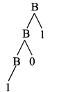
Since , the final denotation is given by . This is precisely the expected result.
5.2 Survey of QPL
The semantics of QPL is based on the idea of annotating a flow graph that represents a quantum program with density matrices for the quantum mechanical parts and tuples of probabilities covering the classical components. Additionally, a typing context is used to keep track of all variables together with their types that are in use at a certain stage of a program.
Since our work is based on QPL, it seems appropriate to summarise its central concepts. The original definition of QPL [Sel04b] provides a more detailed description than given here; an alternative review can be found in [Sch04]. We align our summary on both sources. Note that it is nevertheless useful to have some familiarity with the paper introducing QPL because we can obviously not repeat everything here.
5.2.1 Notational conventions
QPL operates on finite-dimensional quantum states represented by vectors over . The basis states for qbits are defined as and . Combination of multiple qbits are as usual represented by tensor products of these states. Density matrices are used as basis for any manipulations performed by the language. If a state is defined by some vector , the corresponding density matrix is given by and may also be denoted by . Mixed states are represented by linear combinations of pure states, e.g., . Given four matrices of identical dimension, they can be concatenated horizontally and vertically by
| (5.2) |
which is used to specify composite density matrices. This notation is used to specify the semantics of actions possible in QPL which will be introduced in the following sections.
5.2.2 Language elements
QPL programs are given in terms of quantum flow charts44 4 There is also a textual representation for programs, but this is only considered as an aside in the definition of QPL. where each edge is supplemented with all the information necessary to unambiguously specify the meaning of a program. Every edge is augmented with
- ❏
a typing context, i.e., a mapping from identifiers of variables to the types of these. It is written as a list of identifiers followed by their type, e.g., . Typing contexts encapsulating variables which are not related to the present considerations are denoted by .
- ❏
an annotation, i.e., a tuple of density matrices which specifies the state of the system.
The annotation of a classical bit is given by where and represents the probability that the value of the bit is , whereas is the probability that the value is . The annotation for a quantum bit is of the form given by Eqn. 5.2.
All classical operations possible with QPL and their flow graph representations are shown in Figure 5.2. Figure 5.3 depicts the quantum mechanical parts.


5.2.3 Semantics
The semantics of a QPL program can be directly inferred from the flow graph representation. The explicit transformation of a density matrix given in the annotation of the edges serves as a unique representation of the meaning of a program. [Sel04b] proofs that this approach is indeed well-defined and also works for recursion and loops, which can be included into the language. Categorical structures that allow to accommodate superoperators and morphisms to manipulate these according to the possibilities of QPL are used as a formal basis for the definition of the semantics. This categorical superstructure55 5 Note that we are only referring to category theory here, not to the compositional semantics presented by Selinger. is not too interesting for our purposes. It suffices to know that the valuation functions for the diverse language elements are defined as shown in Figure 5.4 and that they indeed fulfil everything which is necessary for a sound and well-defined interpretation. Note that the way how the semantics is specified in Figures 5.2 and 5.3 is not equivalent to the method of Figure 5.4: While the first one relies on explicit transformations of density matrices, the second one uses a more abstract representation in form of superoperators and is almost completely identical to the basis of our approach (the functions computed by both approaches of Ref. [Sel04b] are nevertheless identical except for loops and recursion). Especially, the second variant is compositional, which is a necessary condition to describe multipartite systems in such a way that the description of one part is independent of other parts.

5.2.4 Limitation: Quantum communication
Before we lay out the denotational semantics of cQPL, it is advisable to sketch in which sense the different approaches used in QPL do not work for programs dealing with communication.
First of all, let denote the density matrix of the state shared by Alice and Bob. The information available for each party can be inferred by calculating the partial trace: and . The bipartite density matrix can never be recovered from these partial density matrices because there are many bipartite density matrices which give rise to the same partial density matrices.
One of the goals of denotational semantics is to assign sufficient information to every edge of a quantum flow graph such that the complete semantics of a program can be reconstructed by combining only the information given by the edges constituting the program. The denotation of a statement composed of several sub-statements must be completely determined only by a function of the denotations of the sub-statements.
This is impossible in the annotation-based semantics of QPL because transformations between explicit density matrices are considered. Since a combination of the partial density matrices , which were manipulated by Alice and Bob does not restore the total bipartite state , the QPL annotation would obviously not comply with the physical state afterwards.
A possible solution is the annotation of the complete flow graph, i.e., of both paths representing the control flow for Alice and Bob. In this case, the operations performed by Alice and Bob would be written as tensor products of the type and which act on the complete density matrix . This way, we could assign semantics to the program as a whole, but would loose the ability to construct the denotation of a phrase from the denotations of its subphrases. This means that the semantics of the complete program could not be constructed from the denotation of Alice’s and Bob’s program alone which is in contrast to the key idea of denotational semantics.
Therefore, we need to seek a solution that does not characterise quantum operations by showing transformations of explicit density matrices, but uses something that captures the notion of a transformation in a more abstract sense. Completely positive maps represented by a set of Kraus operators fulfil this need as we will show in Section 5.3.1; this is basically the same approach as used for the compositional semantics of QPL. Nevertheless, QPL does not provide any means of parallel composition, communication and other details which are necessary to describe quantum communication as we will do in the remaining parts of this thesis.
We have presented a quick summary of QPL and the associated
denotational semantics which is based on partial orders of density
operators. Additionally, we have shown why this approach is not
suitable to describe quantum communication respectively the
interaction of spatially separated systems where the combined
density matrix is not available as whole in the framework of the
annotation-based semantics.
††margin:
Summary
5.3 Denotational semantics of cQPL
cQPL is an extended variant of QPL with the ability to express and formalise quantum communication, i.e., the ability to describe multiple parallel flow graphs that exchange quantum and classical information at well-defined points, but do otherwise know nothing about each other. To achieve this, we have to base the semantic description on three components in contrast to the two components (typing context and tuples of density matrices) of QPL:
- ❏
A Kraus aggregation as defined in Section 4.5.4 which is used to keep track of the quantum operations performed on the qbits of the system.
- ❏
A typing context used to specify which quantum and classical variables are allocated at a given moment and which data type they have. This is also important to describe communication because it allows to uniquely determine to which party a variable belongs at a given stage of a program.
- ❏
A probabilistic environment mapping identifiers to values. Since the interaction between quantum and classical parts of the system introduces probability, the values of classical variables are subject to such a distribution. In general, only the range of possible values together with the fact that it is governed by a probability distribution is known in the semantical description.
We refer to these three elements as the three-tuple .
A Kraus aggregation specifies a quantum mechanical operation which has the same effect for all density matrices (in the sense that the application of a Hadamard gate will yield different effects according to the state it was applied to. Nevertheless, it is still a Hadamard gate in every case, and this is the really important thing). Thus, the operation is completely characterised without the need to specify any density matrix at all. This is exactly what is required when spatially separated operations performed by several parties on multipartite states are to be described, as we will see later in greater detail.
To realise the benefits of this approach, consider how the generation of a new qbit in state subsequently followed by the application of a Hadamard gate is described in QPL (we do not show the complete flow graph, but only the relevant parts of the annotation):
Although only the newly created qbit is concerned, the state of the remaining system is still implicitly present in . This is more than needed: It suffices to consider the application of two operations given by the following Kraus sets:
| (5.3) |
where stands for “create a new qbit with label ” and for “apply a Hadamard gate on ”. With these, we can describe the same operation without resorting to a density matrix or any other part of the system unconcerned by the operation at all.
The typing context is basically adopted from QPL. An extension to the framework used by QPL is the probabilistic environment. For every allocated classical variable in the current frame, it is used to specify a probability distribution that maps the variable name to the range of possible values. This distribution is parametrised by density operators because it depends on the initial conditions of the program fragment and on the path taken in the flow graph (an example explaining this will follow in the next section). The probabilistic environment could in principle be replaced by the tuples for classical states as used in QPL, but this works only well for data types with a very low number of bits. Because of this reason, QPL tries to hide these tuples most of the time, so we eliminate them completely and replace them by the probabilistic environment.
The probabilistic environment also deals with quantum variables: For every such variable, the position of the allocated qbits in the global quantum heap is given by the probabilistic environment. This is necessary because quantum variables cannot be characterised by a value as it is possible for classical variables because they do not have a state as such. The state is replaced by the series of operations which have been performed on the variables; since these operations need some location to act on, every quantum variable needs to have a unique position on the quantum heap, i.e., where the qbits are stored.
Note that this approach is somewhat contrary to the spirit of functional programming because it introduces stateful global variables, but a closer examination reveals that QPL implicitly uses the same model and that compile-time checking (and thus the protection against runtime errors) is not affected by this.
In addition to allocated variables, branches in programs are also present in the probabilistic environment. They are identified by a unique ID which is assigned to every branching node.66 6 To be precise: Which is assigned whenever the branching node is transversed because we need to account, e.g., for branches in loops where the same branch might be traversed multiple times. This is necessary because the branching conditions – being based on comparisons of probability distributed quantities – are in general not represented by some fixed values, but represented by a probability distribution as well.
5.3.1 Formal definitions
In this section, we will present some methods to characterise and describe the semantic components of cQPL. Note that in the following, we use to denote the set of all density operators of dimension , dropping the subscript if the exact dimension is not important or can be deduced from the context.
5.3.1.1 Typing context
Let be a list of numbers as given by . is also called the signature of a data type. An associated Hilbert space is given by
| (5.4) |
where is either for quantum or for classical data (cf. Section 4.3.3) where both are distinguished by the index : for quantum variables and for classical variables. The dimension of the -th space is given by for quantum mechanical and for classical variables. Since we restrict ourselfs to finite-dimensional Hilbert spaces, this means that we can use for quantum mechanical and for classical data. To distinguish between both cases, we define the function given by
| (5.5) |
Note that although our formalism allows to define data types which consist of both quantum mechanical and classical components, we do not exploit this possibility because we could not find any reasonable application for this in our work. To keep the formalism as general as possible, we will nevertheless still retain the possibility as long as no noteworthy effort is necessary to do so.
We can define a function to compute the total number of qbits necessary for a given signature ( denotes the cardinality of ):
| (5.6) |
The analogous function for the classical components is given by
| (5.7) |
Finally, two functions and to check if a given data type is purely classical or purely quantum are necessary:77 7 Note that we define a data type consisting of quantum and classical bits, i.e., void, as classical.
| (5.8) | ||||
| (5.9) |
For simplicity, we label data types required for practical use with special mnemonics; some examples can be found in Table 5.1. Note that the type void can, for example, be used to formally describe statements which return no value and thus have no type.
| Mnemonic | Signature |
|---|---|
| bit | |
| qbit | |
| short | |
| qshort | |
| int | |
| qint | |
| void |
Since two finite-dimensional Hilbert spaces and are isomorphic if the sum over the dimensions of their subsystems is equal (this is, e.g., proved in [Wei00, Theorem 2.62]), i.e.,
| (5.10) |
the description of types is not unique. For example, the types given by and are identical and provide only different aspects of the same thing. This equivalence can also be extended to mixed data types:
| (5.11) |
This creates an equivalence class for data types which will be useful in Section 5.3.8. The class of all data types equivalent to is given by
| (5.12) | ||||
| such that |
where denotes the element of the ordered set and is the decomposition of the scalar value into all possible sums given by
| (5.13) |
If , we write .
To illustrate the effect of Eqn. 5.12, consider a data type which consists of quantum and classical bits. Structurally, it does not make any difference how these components are ordered, e.g., is identical with in this sense.88 8 Note that there is a difference between these orderings from the compiler’s point of view because the different components are located at different locations in memory if different orderings are used. The semantics is nevertheless unconcerned by this. Eqn. 5.12 is a generalisation of this idea: The scalar can be decomposed as , and as given by , so there is no difference between any of these groupings. Additionally, it is not interesting how the components are ordered, e.g., is equivalent to . Finally, the quantum and classical components can be arbitrarily interchanged, so we have to consider this as well. The effect of Eqn. 5.12 is to construct all equivalent representations of a data types following these considerations.
Note that QPL uses a Cartesian product of complex vector spaces given by for both classical and quantum mechanical signatures (the set of complex matrices is used to represent the complex Hilbert space of dimension ). This does not reflect the relationship between corresponding quantum and classical objects directly. For example, the data type for bits is given by , whereas for qbits, the definition is ). This leads to appropriate spaces for these objects, but does not present the relation between them directly.
We thus used a different approach that makes correspondences more clear which is important when, for example, quantum variables are measured and the result is stored in a classical variable. Besides, it fits better into the more abstract description of quantum mechanics as introduced in Section 4.3.
Let be the set of finite strings over the alphabet . With this and the notion of types, we can define the typing context used in the semantic description of cQPL.
Definition 5.3.1 (Typing context).
A typing context is a three-tuple where is a set of identifiers in , is a set of types and is a surjective mapping which assigns a type to every identifier. Identifiers starting with must not be used by programs.
Because cQPL is strongly and statically typed (i.e., the type of an expression is completely determined by the types of its components and the type of an elementary component cannot be changed after it has been declared, cf. Appendix B), information contained in the typing context cannot be modified any more once it has been introduced. Note that this does not hinder the possibility of overshading entries. This happens when, e.g., a variable declared in an inner block has the same name as a variable declared in an outer block. Although both have identical names, their types do not need to match because they are otherwise completely unconnected.
Typing contexts are modified when new variables are declared (and thus added to the context) or when variables are removed from the scope (and thus have to be removed from the typing context). Since it is obvious how this influences a given context , we only note that it is easy to define appropriate morphisms which perform the desired job.
Formally, we use the notation
| (5.14) |
to introduce some new identifier with type qbit into the context . Equivalently, the notation is used to remove which is needed to describe sending quantum variables.
5.3.1.2 Probabilistic environment
The probabilistic environment can be defined formally as follows:
Definition 5.3.2 (Probabilistic environment).
Let be a probability distribution on a finite set with probabilities for every element of such that . Let be a set of identifiers, be a set of probability distributions and be a surjective map . Then is a probabilistic environment.
As usual in denotational semantics, the symbol is used to denote an undefined identifier, i.e., a variable which is not present in the environment. To specify components of a probabilistic environment, we use the notation
| (5.15) |
to denote an element of the probabilistic environment where is the identifier, the associated probability distribution and the set of possible values which obviously depends on the data type of . Adding a new binding to a given environment is once more done with the operator which is formally a morphism :
| (5.16) |
Note that multiple inclusion of variables overrides the previous definition. Thus, the meaning of
| (5.17) |
is to create a probabilistic environment which contains as probability distribution for the variable . The previous distribution can then not be recovered any more in .
In direct analogy to Kraus aggregations, probabilistic environments can be combined with ; the summands are prefixed by some constraint that states which one has to be chosen with which probability:
| (5.18) |
where are the conditions which determine the values of and . This construction is necessary for the description of, e.g., if-conditions when it is not a priori determined which path will be selected. If both paths of an if-condition perform a modification on the same variable that already existed before the branch, then the variable will have different values after the merge point. The entries of the probabilistic environment which record this assignment are then prefixed by the branching probability. This is also one of the reasons why the branching probability needs to be kept even after the branched paths are merged again.
Definition 5.3.3 (Distributivity of over ).
The operation is defined to be distributive over , i.e., . This ensures that adding a new binding to a sum of environments results in adding the binding to all contributing environments automatically.
Remark 5.3.1.
Observe that the probabilistic environment is only necessary for classical, but not for quantum variables: The state (or, rather: the history of all operations performed until the present moment) of the quantum mechanical constituents of the computation can be reconstructed with the aid of the Kraus aggregation. Nevertheless, the probabilistic environment is necessary to keep track of quantum variables in a different way which will be introduced in a moment.
Note that the view on quantum variables differs slightly from that on classical ones: It is not only necessary to keep track of the structure of a variable (as is done by the typing context), but also of the position within the quantum heap – this is necessitated by the underlying model of computation as introduced in Section 2.2.3.99 9 The value of a quantum variable can obviously not be directly stored in an environment because the state might be in a superposition. The operations performed on the quantum bit are recorded in the Kraus aggregation and unambiguously specify the state. The environment can be used to provide this kind of information by supplying a map
| (5.19) |
where are integer numbers with and is the size of the quantum heap. The tuple denotes the interval which contains quantum bits. Obviously, the number of qbits allocated in the quantum heap must agree with the number of qbits necessary for the type of the variable as given by the typing context.
In theory, it is possible to assume that the quantum heap can always be partitioned into consecutive intervals; we do not need to take care of issues like fragmentation which does obviously appear in implementations and simulations. We assume that the hardware of the quantum memory take care of this issue by acting like a memory management unit.1010 10 This component of a processor creates a view of the available memory such that every application – roughly – thinks that it would have an own linear address space which is as big as the the one available for the whole system. Note that if the user is allowed to directly address the components of the quantum heap, it is possible to cause run-time errors as in QCL. Therefore, we do not allow this.
Consider a subset of . The set of all interval partitions is given by1111 11 An example might illustrate this definition: Consider the set . This is a proper partition since no elements overlap and the boundaries are adjacent. These conditions can be ensured by considering the last element of the set given by and the first element of the set given by . If the difference between these is , then both the adjacency and no overlap conditions are fulfilled. If this holds for all subsets, we have a proper partition.
| (5.20) |
where we suppose that the contents of all sets is sorted in ascending order. This can be used to formally define how the probabilistic environment can be adapted to the requirements for quantum variables:
Definition 5.3.4 (Quantum part of the probabilistic environment).
Let be a probabilistic environment. It can be extended to fulfil the requirements for the description of quantum variables by the following construction:
- ❏
is extended to where is the total number of quantum bits present in a system. The set of intervals is used to represent quantum variables which reside on the local quantum heap, i.e., which were allocated in the module the probabilistic environment belongs to. is used to denote the originating module for variables which were received from some other party.1212 12 We have to make sure that every quantum bit in the system belongs to exactly one place in a quantum heap. This is simple for single-party programs, but gets more complicated when communicating programs are considered because the case of sending the same quantum bit back and forth between participants must be taken into account.
- ❏
Let be the set of all identifiers for variables with quantum data type. Then, is an injective morphism for which (this ensures that quantum variables do not overlap on the quantum heap) must hold. Then is replaced by in the previous definition.
Note that this definition reflects a fundamental difference between classical and quantum variables: While a classical variable is nothing else than a mapping between an identifier and a value that can be governed by a probability distribution, such a mapping is in general impossible for quantum variables because they do not have a value per se, but only a certain quantum state. To describe this quantum state precisely (disregarding the principal impossibility of implementing a measurement that delivers this information by inspecting a single copy of a quantum system), one would need an infinite amount of classical information because even a simple system such as a qbit takes values in a continuous space as a consequence of quantum superpositions. This makes the classical approach of mapping the identifier to a probability distribution of values impossible. Nevertheless, the quantum variable is completely characterised if its location on the quantum heap together with the operations performed on its initial state are known.
Remark 5.3.2.
Although we retain the name probabilistic environment also for the version of the environment extended to quantum variables, there are no probabilities involved in the connection between variable names and the allocated positions on the quantum heap. The convention just simplifies the notation.
Remark 5.3.3.
Support for mixed quantum/classical types would require a little more effort compared to the case of full separation because with the introduction of such types, the direct decomposability of the probabilistic environment would not be feasible any more. Nevertheless, no fundamental difficulties would be associated with this.
Adding a new quantum variable with name which occupies the quantum heap positions given by is written as
| (5.21) |
Removing a quantum variable is denoted by ; this is required when qbits are transmitted and thus cannot be accessed any more (we drop the index if there is no danger of confusion). Note that there is no need for a corresponding operation for classical variables because overlays provide the required functionality, as will be shown later.
5.3.1.3 Kraus aggregations
We can directly adopt the definition of Kraus operators as given in Section 4.5.4. Nothing needs to be modified for our purposes (note that the composition of two Kraus aggregations was denoted by instead of as used for the other elements of the three-tuple to avoid confusion with the symbol used to combine sub-aggregations).
It is possible to show that this semantic framework can be used to formalise standard QPL, but we omit the details here.
We have introduced the structures which are necessary to
specify the denotational semantics of cQPL; they fulfil the required
properties as described in Chapter 4. The semantic
framework consists of three components: A Kraus aggregation which is
used to store all quantum mechanical operations performed by commands
of cQPL, a probabilistic environment which maps identifiers to
values (possibly governed by a probability distribution) and
provides mechanisms to ensure that quantum variables do not
interfere with each other, and a typing context whose information is
the basis for compile-time correctness checks of programs. These are
grouped in a tuple which will be omnipresent in the
following. Additionally, we have derived some criteria for the
identity of data types.
††margin:
Summary
5.3.2 Some examples
Before we commence to extend the formal definitions for multipartite systems, we want to demonstrate the introduced concepts with some examples which should aid the reader to see the rationale behind their definition.
5.3.2.1 Semantics of sequential programs
Consider the following program fragment which applies a Hadamard matrix to the quantum variable p or q depending on the result of a branch based on a comparison of two classical variables and :
if (x > y) {
   q *= H;
}
else {
   p *= H;
};
The flow graph representation of the fragment is given in Figure 5.5. To shorten the annotation of the edges and to avoid repeating the same information over and over, we introduce the injection functions . are -based injections into the element of an -tuple. If we want to add the contribution to the element of the tuple , we can write this as . The initial tuple of the example flow graphs is abbreviated by ; modifications derived from this are denoted by .

The initial configuration of the 3-tuple is given by (initial list of Kraus operators), (probabilistic environment) and (typing context). We don’t care about their contents in detail, they can represent the semantics of any valid program fragment that might be placed before our example. Things which are of interest for our code fragment are:
- ❏
The two classical variables and , both of type int.
- ❏
The probability distributions which map the variables and to a value contained in .
The probability distribution for classical variables arises because we work with Kraus operators describing quantum operations instead of density matrix transformations. Consider the measurement of a single qbit whose result is stored in a classical bit variable: We know that the range of the measurement outcome is , but we don’t know with which probability the “” and the “” will appear because we do not have an explicit density matrix to describe the qbit. This piece of information can only be gained when the final semantics of the program (in form of a total set of Kraus operators) is “applied” to a well-defined initial configuration; only then quantitative statements about the distribution are feasible. All we know is that the measurement result will be governed by a probability distribution with a certain well-defined range, so we preserve that information.
Since the values of and are given by a probability distribution, the result of the comparison (with outcome range ) can only be specified by another probability distribution which can be deduced from and . Since we need to reference the outcome of the comparison at a later point in the flow graph (when the two edges of the branch are merged), a unique identifier for the node is created ( in this case) and the probabilistic environment is extended accordingly.
Depending on the outcome of the comparison, a Hadamard gate is applied on either or . This does not change the probabilistic environment or the typing context, but is recorded by placing an appropriate Kraus operator in the Kraus aggregation ( and denote the position of the quantum bits in the quantum heap).
After every if-then-else construction, an implicit merge operation which unites the two branches takes place. The probability distribution of the branching condition is preserved in the probabilistic environment under the label assigned to the branch statement; the Kraus aggregation is transformed into a sum that formally resembles a mixed state: With probability (which is the probability that evaluated to true), the operation was performed, while with probability , the operation was .
5.3.2.2 Communication with EPR pairs
Consider the following (pseudo-)code which describes how Alice creates an EPR pair and transmits half of it to Bob:
module Alice {
   new qbit p := 0;
   new qbit q := 0;
   createEPR(p,q);
   send q to Bob;
   new bit b := measure(p);
   if (b) { ... } else { ... };
};
module Bob {
   receive m from Alice;
   new bit b := measure(m);
   if (b) { ... } else { ... };
};
The corresponding flow diagram is given in Figure 5.6.

Note that the labelling formalism is reduced to the basic necessities in this example in order to emphasise the central elements. Because Kraus operators are used to describe the quantum mechanical operations, it is possible to perform spatially disjoint actions by parties who do not know the total state. When the edges are merged together, the operations performed by Alice and Bob can (as was mentioned before) be factorised as , for the combined semantics of both branches; the total density matrix is not involved in this, contrary to annotation-based QPL. The framework to generate the semantics of the total system from the semantics of the components will be introduced in the following section.
5.3.3 Extension to multipartite systems
Since we want to consider the formal semantics of programs which deal with communication, we need to extend the previous definitions to the multi-party case. For this, observe that the number of participants can naturally be assumed to be finite which makes it possible to label each party with a unique identifier of finite length. For formal simplicity, we assume that the set of labellings for participants is disjoint with the standard labels used for variables, i.e., . Let denote the unique label given by the entry of .
Assume that we have communicating parties which are labelled with . According to the principle of compositionality (we will explain this for the context of communication in more detail in Section 5.3.6.4 on Page 5.3.6.4), there is a three-tuple for every participant, i.e., . The combined three-tuple for the complete system is then given by
| (5.22) |
We will consider how the tensor product needs to be defined for each component to provide a sound basis for our further needs.1313 13 Note that although formally, different tensor products are used for each element of the tuple, we use the same symbol for all of them to simplify notation.
5.3.3.1 Kraus Aggregation
Consider, for simplicity, two Kraus aggregations
| (5.23) | ||||
| (5.24) |
(in case of , the shorter list can be padded with zero elements so that can be assumed, but note that it is only for notational convenience). If both lists operate on a disjoint set of qbits, i.e., no send/receive (pseudo-)operations are contained in the lists, then holds. The Kraus aggregation for the composite system can be written as:
| (5.25) |
Note that members of type can be written as . If this is done for all list elements, we see that all combinations of with commute; this induces many equivalent orderings of the lists – in addition to the normal commutative equivalences as given by Eqn. 4.57 for the sublists – which needs to be considered when multi-party aggregations are tested for semantic equality in Section 5.3.5.
Formally, the equivalence class of compatible Kraus aggregations for two independent parallel systems is given by
| (5.26) | ||||
| with |
where the additional constraints on the permutation make sure that the order of and is preserved. We can generalise this approach to Kraus aggregations given in the contracted normal form (padding is applied as usual to compensate for different cardinalities):
Definition 5.3.5 (Tensor product for Kraus aggregations).
Let , …, be Kraus aggregations in the contracted normal form. The tensor product of these is given by
| (5.27) |
Note that the naming of qbits changes when multipartite systems are merged. For Kraus sets which symbolically refer to qbits, the labels must be updated accordingly (the exact renaming scheme is given in Definition 5.3.6). Two aggregations are equivalent if they are member of the same equivalence class as given by Eqn. 5.26 or member of the equivalence class given by the same formula, but induced by a compatible ordering of one or more of as defined by Eqn. 5.25.
Note that we will show in Section 5.3.6.4 how send and receive operations can be integrated into this formalism.
5.3.3.2 Typing Context
Definition 5.3.6 (Tensor product for typing contexts).
The tensor product of typing contexts is given by
| (5.28) |
where denotes a set which contains all elements of prefixed by the unique identifier ; denotes the morphism adapted to the new naming scheme.
5.3.3.3 Probabilistic Environment
The probabilistic environment can be adapted to multipartite systems analogous to the typing context, i.e., by prefixing the variable names with appropriate labels and adapting the morphism used to connect the set of identifiers with the set of data types. Obviously, the prefix for each subsystem must be the same as used for the typing context.
The quantum part needs to be modified as well: The local quantum heaps must be united to a single one; necessarily, the positions of all variables on the new heap still need to be disjoint. This is simple to achieve: If uses the range and the range , the new range is given by and the morphism needs to be adapted such that the mapping remains unchanged for variables originating from and the constant offset is added to its codomain for variables originating from .1414 14 Note that both local quantum heaps could have already used the full number of available quantum bits (); we do not consider this problem any further because it is alway possible to limit the number of quantum bits for communicating systems to because both and are finite. We are not too concerned about this problem because we always assume that there are enough qbits available. The reason behind the restriction to a finite, but fixed number of qbits is to ensure the boundedness of all Kraus operation as explained in Chapter 4. Likewise, the function which associates variable names with quantum heap positions needs to be updated such that the modified variables names are mapped to the modified positions.
We will not consider the renamings any more in the following parts, but just take them as given; this simplifies the notation considerably.
5.3.3.4 Quantum channels
Quantum channels are used to exchange information between processes.1515 15 A user in a real-world implementation is nothing else than a process in the simulation. We thus use both terms interchangeably. Although not only quantum data, but also classical variables can be sent, we restrict our considerations to the first case because the second one is not too interesting from a physical point of view and would only obstruct the view on the central elements. In particular, classical communication can be seen as a special case of quantum communication (cf., e.g., [Key02, Section 6.2.2]), hence the generality of the approach does not suffer from this restriction). Besides, the topic of classical communication has been investigated in classical programming language theory for a long time, so we can refer the reader to the wealth of existing literature about this topic, e.g., Ref. [Rey98].
We have already introduced quantum channels informally in Section 2.2.3.1; here, we consider the concept formally.
Definition 5.3.7 (Quantum channel).
A quantum channel is a five-tuple where is the origin and the destination for a quantum variable (these can, e.g., be represented by processes), is a FIFO1616 16 First in, first out queue. Informally, this is a queue where objects can be put in on one side and taken out on the other side. The object which is put in first comes out first, the second one comes out second etc. containing objects of type , is a morphism to place two-tuples in and is a morphism to retrieve two-tuples from . As usual, represents the density matrix of a quantum variable and the associated type.
Thus, the quantum channel can be used to make sure that not only typing is guaranteed to be preserved along communication (for this, confer further Section 5.4), but also that quantum data does not appear multiple times in a composite system at the same time which is necessary to avoid unphysical situations in the simulation.
Remark 5.3.4.
Note that quantum channels are only necessary when the parallel composition of two or more processes is considered. For single modules, the functions used to deposit respectively request information from the channel together with an abstract representation of the channel (e.g., an identifier) are sufficient.
Remark 5.3.5.
Also note that most descriptions of quantum communication protocols do not consider typing of the exchanged data explicitely, it is nevertheless implicitly implied by the physical realisation of the protocol, e.g., in the measurement process, by the hardware used to realise the communication channel or in the way the quantum part is implemented in general.
5.3.4 Existence of fixed points
Because fixed points are important for the denotational description, we need to prove the following theorem which states a condition for the existence of such. In the following, the condition can shown to be fulfilled for every element of the semantics.
Theorem 5.3.1.
Let be a linear operator acting on a complete partial order with bottom . If is bounded, then a fixed point of exists.
Proof.
Remark 5.3.6.
Note that the same proof could have been deduced at a slightly more abstract level using the notion of a pointed dcpo, i.e., a dcpo with a least element. For structures fulfilling this condition, Theorem 2.1.19 in [AJ94] ensures that the desired least fixed points exist. Ref. [Sel04b] uses a somewhat similar reasoning in the description of recursive procedures where the existence of least fixed point solutions for these is explained by the fact that for Scott-continuous endofunctions on pointed complete partial orders, these always exist.
Remark 5.3.7.
For those who want to be extra sure, the classical fixed point theorem by Schauder which states that any continuous map with a countably compact image on a compact, convex subset of a Banach space has a fixed point could also be used to derive the required property of cp-maps.
We will need fixed points to solve recursive equations which occur in denotations specified by recursive equations. These are required for loops and the combined semantics of communicating systems.
5.3.5 Types of interpretational equivalence
The term “equivalence” is not unambiguous without further specification. Under which conditions can two programs or, respectively, the denotations of two programs be considered as equivalent? QPL has to distinguish between two different types of equivalences as noted in [Sel04b, Section 6.6]; likewise, we can define several types of equivalence:1717 17 Note that our definitions of equivalence do not coincide with the types of equivalence given by Selinger.
- ❏
Two programs are textually equivalent if there is a bijective mapping between the set of all variables the programs use and for every constituent of program A, there is a constituent of program B such that , i.e., the programs are identical already at the level of the syntax. The ordering of these constituents must be identical.
For example, the two program fragments new int a; a:=1; and new int b; b := 1; are equivalent because the sequence of commands is identical if the replacement is applied to the variables.
- ❏
Two programs are denotationally equivalent if their denotations are identical.
The second definition only shifts the problem because it leaves the question of how to identify equivalent denotations. This is problematic for cQPL because we do consider multiple representations of superoperators which have identical effects; some care needs to be taken to exactly specify the meaning of “identical” in this setting. Denotational equivalence can be refined to the following cases for cQPL:
- ❏
Direct denotational equivalence: We can distinguish three different scenarios which exhibit direct denotational equivalence for and given as denotations of :
- 1.
and . This means that both programs have have the same number of Kraus sets as denotation, the probabilistic environment and the typing context contain the same information and the denotations of the statements are pairwise identical.
- 2.
, , , such that the sum of commutator products calculated according to the method given in Section 4.5.4.2 vanish identically, i.e., only permutations with vanishing commutator have been used. This equality holds if only commuting statements have been exchanged to match the lists, the total denotation is thus identical.
- 3.
where means the application of the Kraus set in on where the information contained in is utilised to construct the proper superoperators because the exact representation of in general depends on information given in and . Note that the initial state resolves any symbolic parametrisations which may be present in .
The first condition obviously implies the second and third condition; the second implies the third, but the other direction is not true in general, so equivalences of decreasing strength are defined by this enumeration.
- 1.
- ❏
Heap-permutative respectively variable-permutative denotational equivalence is given if there exists a permutation of the quantum heap positions (respectively the variable names) such that direct denotational equivalence holds. These permutation schemes can be used to align different probabilistic environments to each other.
Note that textual equivalence implies denotational equivalence, but the converse statement is not valid in general.
A last form of equivalence that needs to be considered concerns the parallel execution of programs. If represents a set of communicating modules, the order in which the subsystems are given does not make any difference, i.e., for any and an according update of the references to the other subsystems in for all . Likewise, relabelling of communicating modules does not change the meaning of parallel execution if the reference names in all participating modules are updated correspondingly. This type of equivalence can be referred to as communicative equivalence.
The problem of how to detect equivalence between different representations will emerge several times in the following remarks and is not easy to solve constructively.
We have augmented the definitions of the semantic basis
with the elements required to represent communicating
systems, i.e., cQPL programs which are generally independent of each
other, but can exchange quantum mechanical and classical data in a
well-defined way. Additionally, we have shown that fixed points
exist in this framework; they are necessary to assign semantics to
numerous components of the language as explained in
Chapter 4. Criteria for the equivalence of cQPL
programs were specified as well; this allows to check if programs
which are specified by different sequences of commands have the
same effect.
††margin:
Summary
5.3.6 Semantics of the language components
Chapter 2 gave an informal1818 18 It should be noted that although informal may sound a little fuzzy, such a description is normally the maximal level of accuracy with which users of programming languages (and in most cases, implementors as well) are confronted. introduction the the language elements of cQPL. In this chapter, we will use the mathematical and semantical formalism introduced in the preceding sections to give a rigorous mathematical meaning to these statements. By the compositionality of denotational semantics, this means that all cQPL programs (which are, necessarily, composed of cQPL statements) have a defined semantics. There are two possible representations for cQPL programs in form of textual descriptions and graphical flow charts; we resort to the particular representation that is more convenient for the desired purpose in the following remarks. Establishing a formal correspondence between both possible representations of cQPL is obvious and follows exactly the argumentation used in [Sel04b]; we will thus not bore the reader with details on how to relate both representations uniquely.
Note that we try to keep the purely classical formalism as terse as possible because most problems related with this are not too interesting from a physical point of view. More elaborate descriptions or gentle introductions can be found, e.g., in Refs. [Mos90, Rey98, Win93].
5.3.6.1 Some notational remarks
Some conventions and notations widespread in semantics are uncommon in physics, thus we want to make two short remarks before proceeding further.
Typed lambda calculus
Computer science literature habitually uses the typed lambda calculus (cf., e.g., [RP02]) to formulate the equations for valuation functions; this is useful to not only clarify which parameters are used, but also to determine their type. We, in contrast, use a different notation. Observe, for example, the denotation of the dyadic operator which adds two natural numbers:
| (5.29) |
It is intuitively clear that we are talking about a function which takes two natural numbers as arguments and computes another natural number as result. Nevertheless, we did not formally specify the data types of the arguments nor of the result of the function.
This can be solved by using the typed lambda calculus in which the function would be written as:
| (5.30) |
This very simple example already demonstrates that the representation requires a considerable notational effort. Since nearly all valuation functions for the semantics of cQPL defined in the following require tuples in addition to the effective parameters, this would unduly inflate the length of equations which does not really increase lucidity. Thus, we stick to a simplified notation which follows the algebraic convention for functions as presented above. The domains where parameters originate from are normally clear from the context; we will mention it explicitely should this not be the case since typing is obviously not explicitely part of the simplified description.
Currying/Schönfinkeln
Another point we want to mention is the insight that functions of more than one parameter may always be composed by a number of subsequent functions which take exactly one parameter. Thus, a function with which is an element of can also be seen as a mapping , the parentheses may also be omitted. The technique of transforming a function with multiple arguments into a function which takes only one argument, but returns another function which requires the remaining arguments and returns the result is conventionally termed currying, although it was first introduced by Schönfinkel [Sch24]. The process can obviously be repeated so that there are only functions left which take exactly one argument. In the following, we will use the form which is more apt for the respective purpose.
5.3.6.2 State transformations and fixed points
Valuation functions for top-level elements of cQPL (i.e., those for expressions) work on a three-tuple and produce a new three-tuple as we will see in the course of the following remarks. Thus, these tuples form the domain which is the basis of semantics. Since we will need fixed points as solution of several recursive domain equations, we need to show how to calculate them for tuples. We have already shown that fixed points exist for Kraus aggregations which fulfil certain conditions. Now, we need to transfer this to tuples.
For this, note that the typing context is not involved in the calculation of fixed points: Its purpose is to ensure well-typedness of programs (which will be explained in more detail in Section 5.3.8) and (as a consequence) to make sure that ownership of qbits is unique. Otherwise, it has no semantical meaning.
To consider the contribution of the probabilistic environment, observe that we could do without it in principle by using a different notation as is, for example, the case in QPL (we did not adopt this approach because it quickly leads to very long annotations which are cumbersome to handle; additionally, our approach has a greater similarity with the standard notation commonly used in denotational semantics). For every possible value of a variable in the probabilistic environment, a specific Kraus aggregation can be inferred. Consider a measurement of two qbits whose result is stored in a classical variable of two bits. A probability distribution is stored in the probabilistic environment where represents the information that the quantum variable contained in the typing context was measured (this will be covered in more detail in Section 5.3.6.4 on page 5.3.6.4). Since the exact form of the probability distribution depends on the state of the measured variable about which nothing is known in the worst case (if, e.g., the variable was received from a remote party which did not characterise it any further), we have to account for all possible cases, i.e., for all values the variable can have in principle. Let be the contents of the Kraus list K from the tuple immediately after the measurement where denotes the Kraus set for a projective measurement. This list can with the help of the probabilistic environment be rewritten into a four-tuple
| (5.31) |
where is one of the projection operators which constitute the POVM elements of the measurement. Note that the Kraus aggregations contained in tuples of this kind are always unparametrised.1919 19 This kind of split is one of the reasons why it is more convenient to work with Kraus representations of cp-maps instead of the cp-maps alone which would also be possible in principle.
If there is now an operation performed which is independent of the measured variable, the contribution to the Kraus set is appended to all list components in this picture. Consider, for example, the application of some operator to another quantum variable . The resulting four-tuple of Kraus aggregations then looks like:
| (5.32) |
The first entry belongs to the case that , the second to , and so on. Obviously, it is much simpler to write this in our notation as
| (5.33) |
from which the tuple representation can be reconstructed. This also works if operations are considered that depend on the state of a classical variable governed by a probability distribution. Consider, for example, the case that an operator is applied to some quantum variable if the value of is (the program code for such an operation would be if (x = 2) then v *= U;). In our notation, the branching condition is preserved in the probabilistic environment as shown in the example given by Figure 5.5. From this information, the corresponding tuple representation
| (5.34) |
can be constructed. Note that is only applied in the case .
The transfer from our representation to tuples of Kraus aggregations is easier when classical variables with defined values and no associated uncertainty are considered, so we will not show an explicit example for this.
As the forgoing considerations have demonstrated, the probabilistic environment and the Kraus aggregation contained in the tuple can be used to construct a tuple of Kraus aggregations where the tuple contains one entry for every combination of values the classical variables can be in. Fixed points of triples must therefore be calculated separately for all possible Kraus aggregations that can be constructed from the triple because each of them represents another possible meaning of the program. This is possible with the methods introduced before. After the fixed points have been derived, the usual representation can be used again. Thus, calculation of fixed points effectively only requires the properties of Kraus sets as introduced before. In the following, we need thus only make sure that the conditions for the existence of fixed points of Kraus aggregations as given in Theorem 5.3.1 are fulfilled to ensure the existence of fixed points for tuples.
5.3.6.3 Classical operations
The classical subsystem of cQPL consists of the following parts:
- ❏
Allocation and (implicit) deallocation of classical variables.
- ❏
If-then-else expressions.
- ❏
While-loops (this and the previous point require the evaluation of boolean conditions which must also be accounted for by the semantics).
- ❏
Sequential composition.
- ❏
Do-nothing-operation (skip).
- ❏
Sending and receiving of classical states.
- ❏
Assignment to classical variables.
- ❏
Calling procedures which manipulate classical data.
- ❏
Blocks.
Note that we do not cover sendig and receiving of classical data because this has extensively been covered in the literature. Additionally, it is in principle always possible to achieve the same effects with the transmission of quantum mechanical information. In the following, we cover only the valuation functions which are either absolutely indispensable or are influenced by the quantum properties of our language.
Sequential composition
Modifications made to the typing context, the probabilistic environment and the Kraus aggregation made by the first statement must be taken into account when the semantics of the second statement is calculated:
| (5.35) |
This is utilised many times in the denotational equations for quantum communication.
Blocks
Blocks are used to introduce multiple levels of scope into programs. This can happen both implicitly (e.g., in loops) and explicitely (by syntactical specification of blocks), but there is no need to distinguish between these cases from a denotational point of view.
Superficially, a block looks just like a collection of multiple statements which are executed one after another; but some additional points need to be taken into account:
- ❏
New variables (both quantum and classical) may be declared inside blocks, but they cease to exist once the block’s scope is left.
- ❏
New variables do overshade old ones if they share the identifier.
- ❏
Changed bindings of already existing variables are also visible after the control flow has left the block’s scope.
Thus, the probabilistic environment is partially affected by a block. The typing context before and after the block is identical and thus unaffected by the block’s effect,2020 20 But note that the typing context within the block may well be different than the one outside. and the Kraus aggregation records everything that has been done inside the block.
Conditionals and Operators
Dyadic operators combine two subexpressions into one result, as, e.g., all arithmetic operations do. Conditionals are operators which result in a boolean variable, i.e., they evaluate to one of the values true or false which are represented by and . In contrast to most classical languages, the result of both types need not be fixed with certainty, but can be governed by a probability distribution. Note that conditionals may not be used as stand-alone expressions, but can only be part of conditional statements. This is why their semantic valuation does not result in the usual tuple, but in a probability distribution for the possible results which is, e.g., apt for inclusion into the probabilistic environment. The basic valuation functions are given by:
| (5.36) | ||||
| (5.37) |
where and . The meaning of the operations is defined as usual, but the probability distribution nature of the arguments needs to be taken into account:
| (5.38) |
This expression results in a new probability distribution that can be used by the elements further up in the evaluation hierarchy.
Note that the denotation of a single variable is given by the corresponding probability distribution which can be found in the probabilistic environment:
| (5.39) |
This definition ensures that chains of expressions using dyadic and monadic operators (e.g., ) are covered by the semantics because and in Eqns. 5.36, 5.37 can either be values or other operator expressions.
Also note that the eventual action of the respective operators (, , …) can be seen intuitively, so we abstain from further formalisation and rely on the reader to use his common mathematical sense.
Remark 5.3.8.
Note that we do neither consider any problems of numerical accuracy nor of limited ranges of representable numbers for the specific data types. Consequently, we also do not care for the problem of division by zero. We are aware that such pitfalls exist, but are not interested in their solution in this context since their nature is purely classical.
If-Statements
The semantic description of the if-statement is simplified by introducing the following helper function:
| (5.40) | ||||
which eases selection of components of tuples gained by other evaluations and additionally circumvents repeated semantic evaluations of some components. The tuple is the result of the evaluation of the if-branch, while is for the then branch. is the probability distribution governing the branch, and is the identifier which is used to represent this distribution in the probabilistic environment. represents the Kraus aggregation that contains only the elements that were appended to in comparision to ; this ensures that only new contributions introduced in the branches are added to the Kraus aggregation finally. The denotational description for the if-statement then reads as
| (5.41) |
where uid is a unique identifier for the branch which can be chosen at will, but must not be identical with other identifiers already in use. Such a choice is simple for non-communicating programs. The extension to communicating systems is possible if every identifier is given a unique prefix for each partner as described before.
Note that although dyadic operators might syntactically be used to describe arithmetic operations and not necessary conditionals, this source of mistake is ruled out by the type system which only allows boolean typed expressions for .
While-Statements
While statements can be solved using the fixed-point theorem given in Eqn. 4.4.1. For this, note that the denotation of the while function can be rewritten using the previously considered if-function together with an explicit block ( denotes a boolean condition and a statement):
| (5.42) | ||||
| (5.43) |
Eqn. 5.43 is a recursive equation ( appears both on the left hand and the right hand side) whose solution is a fixed point. The agreement is that the least fixed point is taken to be the denotational solution, and this is exactly what the fixed point theorem delivers. To write this formally is now a standard exercise of denotational semantics [Rey98, Mos90], but we show it nevertheless because it is an instructive example for the technique of solving recursive equations which will be necessary for the denotation of quantum communication. Consider the function given by
| (5.44) |
Then the fixed point solution can be formally written as
| (5.45) |
where is any tuple as usual; assume that is defined like
| (5.46) |
since we have to account for the case that the argument of is because of the recursion (note that we would have to use two different symbols for to write this überproperly).
Assignments
Assignments in cQPL can be seen as a convenience mechanism which extends the simple binding of identifiers to values; it is not necessary to introduce the concept of stateful variables to the language to be able to formalise assignments. The description can be simplified if some syntactical transformations are applied. For this, first consider the following program fragment:
new int a := 10;
// Do something using a (part 1)
a := a + 4;
// Do something using a (part 2)
The assignment is equivalent to introducing a new identifier a’:
new int a := 10;
// Do something using a (part 1)
new int a’ := a + 4;
// Do something using a’ (and replace all a by a’) (part 2)
This strategy also works when blocks are taken into consideration:
new int a := 10;
if (...) {
  new int a := 5;
  a := a + 1;
  ...
}
else {
  new int a := 1;
  a := a + 1;
  ...
}
Note that not possible to employ a static renaming scheme in this case because the identifiers a in both subsequent blocks would then end up with identical names which leads to problems. We thus have to postulate that new identifiers are always chosen such that they do not overlap with previous identifiers and must, of course, also not overlap with identifiers which can be assigned by the user. This is possible if the set of identifier strings is denoted by , we introduce a second set of strings with ; each time an identifier is overshaded, it is replaced in its complete scope with a new one in that has not been used before. While this policy is hard to implement in practice,2121 21 This is exactly the reason why mechanisms like call-by-name disappeared as a curiosity some thirty years ago. it does not present any problem in theory (even cases which require an infinite number of replacements are no problem because there are infinitely many unique identifiers).
Most important, the approach is also valid when loops are introduced because these can be rewritten using a (possibly infinite) chain of appropriate if-then constructions as is done in the denotation of them.
In conclusion, we do not need to take care for the obstacles introduced by overshading, but can simply ignore the problem in the denotation of assignments ( denotes some identifier):
| (5.47) |
where is some arbitrary arithmetic expression (which includes single identifiers); the denotation of this is obvious and will not be considered further. Note that this valuation function does not cover the case that the result of a quantum variable measurement is stored in a classical variable; this will be covered later when we describe the denotation of the measure funtion on Page 5.3.6.4.
Allocating and destroying variables
As we have noted in the previous remarks, we do not need to take the problem of overshading into account when dealing with assignments; this obviously also applies to allocations. We refrain from a more detailled description of this topic because everything necessary for the solution can be readily found in the literature, e.g., [Win93, Rey98, Mos90]. Note that allocating new variables does not present any problems for the boundedness of the Kraus aggregation because the number of qbits is limited by , an arbitrary, but finite quantity.
Procedure handling
Procedures in cQPL follow the standard scheme of classical languages for the non-quantum part. The denotation of such can therefore be directly taken from the usual textbooks [Rey98, Mos90, Win93], so we will not repeat this here. The interesting problem is given by recursive procedures, especially when they act on quantum parameters. For simplicity, we consider directly recursive procedures with quantum parameters; the case of indirect recursion is in princple identical, but necessitates more formal effort, so we skip it here. The solution is an adaption of the method presented in [Sel04b, Sections 5.5 and 6.5] for our purposes.
Consider a procedure which depends on itself, e.g.,
| (5.48) |
If is given as a flow chart, this can be interpreted as shown in Figure 5.7: A “hole” in the representation of is replaced by with another hole, this is again replaced by the same, …

proc rec: test:qbit {
  A
  if (cond) call rec(test’);
  else { ... }
  B
}
Formally, we can thus define an approximation relation given by
| (5.49) |
where are approximations of which get better with increasing . is the crudest approximation which simply does not terminate. The solution of Equation 5.49 is another case for the fixed-point theorem. Once a solution for has been found, it can be applied to any tuple to calculate the required state transformation. Note that although the procedure depends only on quantum variables, there nevertheless needs to be a termination condition. In the example, this condition is given by the if-then-else statement in which the recursive call is wrapped; since the procedure only takes a quantum parameter, the condition is either trivial or depends on a measurement of quantum states. In the first case, the condition depends only on classical variables which were allocated within the procedure, the condition could thus be determined at compile-time and the recursion unrolled because the recursion depth is already known. In the second case, we really need to unwind the procedure.
5.3.6.4 Quantum operations
The quantum mechanically relevant operations of cQPL are :
- ❏
Application of (unitary) operators.
- ❏
Calling procedures which manipulate quantum data.
- ❏
Sending and receiving quantum states.
- ❏
Measurements.
- ❏
Creating new and destroying existing quantum states, where the last operation is not explicitely, but only implicitly possible when quantum variables drop out of the present frame. Sending quantum variables makes them disappear from the scope so that they can not be accessed any more, but does not destroy respectively deallocate them.
We will give formal denotations for these constructs in the remaining part of this section. Obviously, the description of communication is our foremost concern, so we elaborate this in most detail.
Unitary operators
Unitary operators induce isometries, so the corresponding Kraus set is obviously bounded and filfills the requirement for fixed points. Every unitary transformation can be expressed by a Kraus set with only one element. The semantics of a unitary transformation acting on the qbits is given by
| (5.50) |
Note that the type system ensures that the variable/operator dimension on both sides of the expression matches as required, i.e., the classical variable has the proper size to hold all potential measurement outcomes.
Measurements
Measurements are described by the following semantic equation:
| (5.51) |
Hereby, denotes the function to generate the set of projectors for the type of which can be resolved from the typing context . The required basis for the projection (which is actually nothing else than the basis for in Dirac notation, also named the standard basis) is given by
| (5.52) |
The corresponding Kraus elements are obvious. Accordingly, denotes the probability distribution which connects the possible values of with a probability distribution induced by the projectors. Since the measurement operators work on discrete states in a finite-dimensional Hilbert space, they are obviously bounded.
Remark 5.3.9.
Note that although we restrict measurements to projections onto the standard basis, projective measurements in arbitrary bases can be realised by applying appropriate unitary transformations prior to the measurement.
Sending and receiving qbits
To consider sending quantum variables, we first split commands which send lists of quantum variables into a list of commands that send one quantum variable each:
| (5.53) |
The denotation of a single send command is given by
| (5.54) |
is not a real physical map as other cp-maps are, but only a “placeholder” to note that qbits have been sent. This will become important when the semantics of parallel execution is considered further below. The interesting thing here is that the sent qbit is removed from the typing context and from the probabilistic environment. Thus, it is not visible any more in the remaining statements. Further access to it can be detected as erroneous at compile time; the typing context gives the formal basis for this.
Receiving qbits is described in a similar manner. First, a receive operation with multiple quantum variables is split into a sequence of single-variable receive operations:
| (5.55) | ||||
The denotation of a single-variable receive command is given by:
| (5.56) | ||||
Again, is a placeholder required to denote the semantics of parallel composition.
Parallel composition
The compositionality principle of denotational semantics implies that the formal denotation of sending and receiving qbits must be independent of the conjugate action, i.e., sending must be independent from reception and reception must be independent from sending. This is fulfilled in the formalism of cQPL as we have shown on page 5.3.6.4. Nevertheless, the denotation of the communication as a whole requires (at last) two communicating partners. It needs thus make use of both of them to assign semantics to communication.
Before we start with the formal details, we want to motivate why parallel composition is necessary at all. For this, consider the case of two processes where sends a quantum bit (which we call ) to and, later on, receives a quantum bit from (which we call ). We must distinguish two different cases (note that for more difficult cases with an arbitrary number of send and receive statements, the conditions become more complicated because we need to account for more general schemes of mutual influence. These conditions will be developed stepwise in the following):
- ❏
The returned quantum bit was not identical with the sent one, . The inequality refers to the positions occupied by the qbits on the combined quantum heap, it is not related with the names of the qbits.
- ❏
returned the quantum bit it got from , .
Consider the consequences for the semantics of parallel composition when the interaction of both processes is considered (both cases can be treated identically if only the separated semantics is taken into account): While in the first case (), operations on and end up on different physical locations, the same operations must in the second case () be applied to the same physical location. Therefore, we must be able to construct enough information from the composed systems such that it is possible to distinguish between both cases.
Additionally, the distinctness of qbits influences denotational equivalence; many different orderings of the actions performed by and lead to the same semantics (the exact conditions for this will be formulated later on), but the class of possible reorderings is usually bigger if there was no interaction on the same physical location in communicating modules. Figure 5.8 presents a visualisation of this fact using a pseudo flow diagram.

There is no explicit statement in the syntax of cQPL which describes the combination of two processes. As explained in Chapter 2, communication is realised implicitly using modules which interact among each other. These modules must thus be given some semantical meaning; this will be developed in the following. Note that we restrict the description to two communicating processes which we call A and B (this might stand as an abbreviation for the omnipresent Alice and Bob) at first. Consider the following cQPL fragment:
module A {
...
};

module B {
...
};
Any valid cQPL code (except the definition of new modules) may be contained in the bodies of module A and module B; both entities thus constitute regular cQPL programs whose meaning is made up by the meanings of all statements they consist of. Thus, we can write and for the denotation of the code as if the modules were regular, uncommunicating cQPL programs.
To consider the communicative interactions between both, we introduce the operation
| (5.57) |
where denotes the inital tuple without content. The valuation function is used to compute the combined denotation of and which we also call parallel execution. It must obviously only depend on the denotations and , i.e., tuples. Since we do not want the semantics of communication to depend on the order in which the communicating partners are specified, the operator must necessarily be commutative: . This equivalence can easily be achieved: It suffices to define the operator in such a way that the modules are ordered lexicographically, then the order in which they are specified does not influence the denotation; the commutation relation is thus automatically fulfilled.
is used to evaluate a semantic equation with empty initial context; this is obviously the case when the top-level of a program is considered (as is the case for modules) where no definitions can have been made yet. Thus, .
Consider the evaluation of and which both do as usual depend on tuples. results in the creation of a valuation function which depends on the tensor product of these tuples, i.e.,
| (5.58) |
Both representations convey the same information. This is immediately obvious if the expressions are written as direct -abstractions as defined in Section 5.3.6.1 together with an appropriate “untensoring” function which separates the tensor product of the combined tuple into two components. We will not show this explicitely to avoid introducing even more symbols.
Note that termination of and alone does not imply termination of .2222 22 Here, the question arises how termination should be defined for communicating processes if only one part (A) of a total system is considered. We could, for instance, define a demonic partner which always supplies the required number of qbits the process needs and absorbs any number of qbits sent, but this will not necessary lead to termination of A. The exact solution of the problem depends on the context in which it is considered; we will not deal with it any further here, but define a process as terminating if there exists a demonic partner that behaves in such a way that the process terminates. This can be seen by considering the following simple program:
module A {
  new qbit q1;
  send q1 to B;
};
module B {
  receive a1:qbit from A;
  receive a2:qbit from A;
};
While both processes represent valid cQPL programs, they will obviously result in some non-terminating program (which should thus denote ) because will wait forever for the second qbit () to be sent. Thus, is possible although both and .
Extensions of the semantical components to the multi-party case were defined in Section 5.3.3; they provide the basis for the denotation of parallel execution which will be developed stepwise by considering bipartite systems without communication, bipartite systems with single send/receive pairs, bipartite systems with arbitrary send/receive statements and finally, arbitrary multipartite systems.
Thus, let A and B be two programs which do not use any communication. The semantics of their parallel execution can be readily denoted:
| (5.59) | |||
Note that the following equivalences hold if are parts of a program which do not contain any send/receive operations (we omit the required s in the second line to simplify the notation):
| (5.60) | ||||
| (5.61) |
This ensures that it does not make any difference if we consider the sequential combination of two parallel executions or the parallel execution of two sequential combinations as shown in the formula; we will make use of this later on.
The situation gets more complicated if a single send/receive pair is allowed, i.e., if a single quantum variable can be transferred from A to B (the case B to A is nearly identical, so we restrict ourselfs to the first case). Let and denote the Kraus pseudo-operations for sending and receiving. To see how these operations influence the possible equivalent compositions of a program, observe the following two schematic Kraus aggregations:
| (5.62) | ||||
| (5.63) |
To consider how these aggregations can be rearranged, we define the following function:
| (5.64) |
Remark 5.3.10.
The same effect could have been achieved with the standard commutator in principle, but we want the notation to emphasise additionally that not the simultaneous diagonalisability, but the fact that the operations work on disjoint bases is responsible for the exchangeability. Additionally, using the standard commutator to show equivalence between permutations of communicating systems would have interferred with the standard permutation rules that would then have become more complicated.
Since the two processes are necessarily totally uncorrelated before the transmission takes place, the parts given by the sub-aggregations
| (5.65) | ||||
| (5.66) |
can be composed as in Eqn. 5.59 because . Since the parts after sending respectively receiving the quantum variable are uncorrelated as well (they both work on disjoint sets of qbits; this property remains valid in the combined semantics because the combination of the probabilistic environments creates an appropriate combined quantum heap as described in Section 5.3.3), the sub-aggregations
| (5.67) | ||||
| (5.68) |
can likewise be parallel composed as in Eqn. 5.59. The only thing which needs to be taken into account is that references to the position of the received qbit must be replaced by the position of the qbit on the combined quantum heap in the combined probabilistic environment. This can formally be achieved by the following function (here, denotes a send and a receive statement):
| (5.69) |
Here, denotes the usual parameter tuple with the additional requirement that it must have the structure which is gained by combining two tuples with a tensor product as given in Section 5.3.3. itself is responsible for two things: On the one hand, it applies the effect of to the parameter tuple, and on the other hand, it replaces the portion of which contains the information about the received quantum variable so that it now points to the position of the sent quantum variable on the combined quantum heap; the resulting probabilistic environment is denoted by . This is obviously possible since does have access to the information provided both by send and receive. To illustrate the effect of , consider the following example: Let the sent quantum variable be denoted by q and the received one by r. The names of these variables will have thus been changed to and . The receiving module does not have any information about the received quantum variable except its type and its local name; the position on the combined quantum heap is unknown. This can now be changed by ; for that, it inserts the position of on the combined quantum heap into the combined probabilistic environment such that points to it. Nothing more is necessary to identify the received quantum variable with the sent one.
Note that defines the analogous function for the receive/send case. This is necessary when bidirectional communication between processes is considered. Except the inverted direction of data flow, the function is completely equivalent to .
Thus, the semantics of parallel execution for processes with a single send/receive operation can be reformulated as
| (5.70) |
where and denote the parts of the program which induce the operations described by as given by Eqns. 5.65–5.68. It is already known how to compute the semantics of . To compute the denotation of the complete statement, we first consider how to include the send/receive pair into the description:
| (5.71) |
Note that although with argument appears both on the left and right hand side of this equation, it is not truly recursive, but can here be seen as just a breakdown into simpler cases. A general recursive formula will be derived in the following.
By using Eqn. 5.70, we can now give the denotation of the complete parallel composition as defined in Eqn. 5.61; for this, we define the righthand side of Eqn. 5.71 to be denoted by to increase clarity:
| (5.72) |
Note that establishing the semantics of a given description is one thing we need to do; finding equivalent descriptions for a given communication is another task. For this, we need to consider all rearrangements that preserve semantics. This allows us to decide if two communicating programs are identical because we can check if they can be brought to the same form.
For the case of a single send/receive pair, the operations can be shifted in the Kraus aggregation if certain conditions hold:
- ❏
The send operation can be postponed to the end of the aggregation (at least in the case where no more send/receive operations take place) or brought forward by positions in the Kraus aggregation if .
- ❏
The receive operation can be brought forward to the first position of the Kraus aggregation (again, this relies on the fact that only a single send/receive operations takes place) or postponed by positions if .
Performing shifts characterised by these operations together with reorderings as given by Eqn. 5.26 generates the equivalence class of all programs with a single send/receive pair that posses the same semantics.
The next step is to include arbitrary send/receive operations into the communication between and . As in the case of a single send/receive combination, the send/receive statements act as synchronisation points; the denotation needs thus be aligned along them. The problem to solve is now given by
| (5.73) |
First, we will establish the semantics for the given ordering; semantics-preserving permutations will be considered afterwards.
Note that we only consider the denotation of data flow in one direction for simplicity; the semantics of the case which may appear mixed with the other form is gained by replacing with at the appropriate places). To find a solution for this equation, define
| (5.74) |
Eqn. 5.73 then has the form
| (5.75) |
According to Eqn. 5.72, the solution of Eqn. 5.75 is given by
| (5.76) |
By introducing as abbreviation for the part following and expanding to , the formula reads as
| (5.77) |
This type of equation is already well-known; it can be further resolved to
| (5.78) |
By recursively defining
| (5.79) | ||||
| (5.80) |
we see that the final solution of Eqn. 5.73 is given by
| (5.81) |
where needs to be expanded as defined above.
The whole process thus leads to a recursive valuation function given by
| (5.82) |
whose solution can be found by resolving the recursion in the usual way.
Now, consider which alternative orderings of the Kraus aggregations preserve semantics in the multi send/receive and receive/send case. For this, observe the following symbolic representation of two Kraus aggregations (to save some notational effort and to increase lucidity, we represent the Kraus sets which are not concerned with communication by boxes. Although the boxes have identical widths, they do not need to contain the same number of Kraus sets):
| (5.83) | ||||
| (5.84) |
As in the case of a single send/receive pair, we know that the blocks and (considering again the compatible displacements of and ) can be arbitrarily combined because they work on disjoint subsets of the quantum heap; the same holds for and . In addition to the previously given rules, the following restrictions hold for shifting send and receive operations in multi send/receive scenarios:
- ❏
Two consecutive send statements can only be interchanged if the corresponding receive statements are interchanged, and vice versa.
- ❏
If the blocks and can be taken like single blocks when possible orderings according to Eqn. 5.26 are considered. Note that the validity of this condition can only be detected if the combined quantum heap is considered. If it holds, then the sender does nothing to the sent and the receive does nothing to the received quantum bit; thus, the statements contained in the blocks can be executed in arbitrary order.
Two systems are identical if their denotations can be unified by performing rearrangements according to these rules.
Another possibility that needs to be considered is the case where the number of send/receive pairs in the parallel processes does not match. As we have described before, this leads to a non-terminating process because either the sending process wants to ship a quantum variable, but cannot deliver it and thus blocks or the receiver wants to get a variable, but blocks indefinitely because there is no sender for one. The semantics should thus be given by for both cases.
For the case of two parties (where we do not need to consider the case that a balanced number of send/receive statements is present, but the distribution among the parties is unmatched), this is covered by the following definition:
| (5.85) |
where denotes the number of send and the number of receive statements. The denotations and are supposed to be those derived for the parallel composition. The extension to higher-dimensional systems is obvious, so we omit it here.
Finally, we can describe the semantics for multi-party communication with arbitrary send/receive statements which is the most general case and therefore includes everything considered before. The problem which needs to be evaluated is given by
| (5.86) |
where (note the different notation compared to before!) represents all statements given in module ; this may contain any number of send/receive statements that are now denoted by and where is the receiver for and destination for and the sequence number within the other send/receive statements of the communication channel the statement works in (if we consider for example three parties , and , then there are the channels –, –, –).
The semantic context the evaluation is based on is given by the tensor product of the semantic contexts of the subsystems, i.e., and equivalent for the initial context. The valuation function given by Eqn. 5.57 can be extended from the two-party case to the -party case without any problems, we denote this by . Since communication still takes place between two partners (although there are now many choices for such two-partner subsystems), there is always a pair of corresponding send/receive respectively receive/send statements. To take the -dimensional semantical context into account, the definition of (the version for two parties is given in Eqn. 5.69) needs to be adjusted as follows when sending a quantum variable from system to system is to be covered:
| (5.87) |
is again responsible to apply the effect of to the parameter tuple; note that in this case, do-nothing-operations are used for all systems except and because these are not concerned with the communication. This is to ensure that the dimensionality matches.
Additionally, replaces the portion of which contains the information about the received quantum variable so that it now points to the position of the sent quantum variable on the combined quantum heap. This is identical to the effect in the simplified case for two systems. If in this case the sent quantum variable is denoted by q in system and the received one by r in system , then the names of these variables will have been changed to and . simply inserts the position of on the combined quantum heap into the combined probabilistic environment such that points to it.
With this, we can generalise the recursive definition of Eqn. 5.82 to the case with an arbitrary number of participants:
| (5.88) | ||||
Finally, this is the solution to the most general case of communication which can be expressed in cQPL.
5.3.7 Explicit transformations of density matrices
Although the abstract view on quantum operations which we have presented in this work is quite suitable for reasoning about general formal properties of quantum systems, the demands of practical work are usually of a different nature: Here, one is interested in the calculation of explicit states and probabilities which determine a system and allow predictions about its past, present and future behaviour. This goal is usually achieved by specifying the initial state of the system, subjecting this to diverse transformations and measuring the required properties which give rise to the desired explicit probability distributions.
The semantics of a cQPL program can be used to generate exactly this information: The abstract transformation given by the semantical denotation of a program is a function which maps the density matrix of the input state to the density matrix of the output state. Obviously, the election of a certain density matrix as initial state implies loss of generality, but in turn allows to infer real-world information, not just abstract properties of generalised systems.
5.3.8 The type system
Typing judgements make statements about the connection between expressions and their types; cf., e.g.,[Car97] for an introduction. For our purposes, the following two building blocks are necessary to describe the properties of cQPL:
| (5.89) | ||||
| (5.90) |
Proper typing is necessary to eliminate certain runtime errors by applying appropriate compile time checks (cf. Section 5.4). Additionally, it is the key to showing that our formalism ensures that quantum bits can – especially in communicating systems – be only manipulated by one party at a time (a similar line of reasoning, albeit for a quite different formalism, was used in [GN05]). The typing context provided by in the tuple is the basis for this.
Properties of the type system are customary expressed with judgements of the following general form:
| (5.91) |
where the are called the premises and the conclusion. If all premises are true, the conclusion is fulfilled. Such judgements can be used to deduce the type of a given composite expression in an automated, formal manner. The following elementary typing judgements hold for cQPL:2323 23 Remember: ensures that the data type of is purely classical.
| Scalars | (5.92) | |||
| new t n := v | (5.93) |
| (5.94) | ||||
| Conditionals | (5.95) | |||
| Arithmetic | (5.96) |
Again, we do not consider division by zero or overflows; up- and downcasting of data types and procedure handling is also skipped. An equivalence relation between two types was given by Eqn. 5.11 in Section 5.3.1.1; this can be immediately carried forward to typing judgements:
| (5.97) |
Note that we do not consider these equivalences explicitely in the following to simplify the notation, all statements are automatically supposed to hold for all equivalent types as well without further noting this.
Also note that subtyping (i.e., considering one type as a subtype of another and allowing appropriate conversions) is not explicitely taken into account because this is also a problem which is specific to the classical data types of cQPL and thus not of too much interest here.
5.3.8.1 Quantum variable tuples
Tupling of variables must make sure that no component appears more than once in the list because this would allow to write programs which violate the no-cloning principle and thus lead to runtime errors. Formally, the requirement is given by2424 24 Remember: ensures that the data type does not contain any classical components, denotes the positions in the quantum heap occupied by a quantum variable.
| (5.98) |
The meaning of this is as follows: formulates the requirement that all variables are well-defined. The condition requires that all components are quantum data types; the tuple thus has no classical components which is justified by our abdication of mixed types. The condition is a formal version of the requirement that no variable may appear more than once in the list of variables. The conclusion which can be drawn from these premises is that is a proper quantum variable tuple, i.e., a well-typed expression in the current environment.
5.3.8.2 Application of operators
The application of unitary operators requires that the dimension of the operator matches the dimension of the variable or variables it is applied to. Formally, this is written as
| (5.99) |
The statement additionally ensures that the typing of the qbits involved is not influenced by the operator application. Note that we do not explicitely specify a formal condition for the unitarity of an operator given in terms of a function of its components. The membership in is sufficient for our purposes. The distinctness of the destination variables for the transformation is already ensured by the tupling requirements given above, so it does not need to be checked explicitely.
5.3.8.3 If conditionals and while loops
The condition for this construction must have type bit, whereas both possible paths must be well-typed:
| (5.100) |
A similar condition holds for the while loop:
| (5.101) |
5.3.8.4 Measurements
The classical data type used to store the result of a measurement must have the same number of bits as there are qbits in the quantum variable. This is represented by the condition
| (5.102) |
5.3.8.5 Communication
Sending qbits
When qbits are sent, the type system has to make sure that no qbit is sent twice because this would result in the same effects as if operators could be applied to multiple copies of the same qbit; using a tuple to combine the sent qbits automatically solves this problem:
| (5.103) |
Note that the type system is not concerned with the actual receiver of the qbits; this information is only required for the denotation of the expression, but not to ensure well-typedness.
Receiving qbits
When qbits are received, the type system must make sure that the destination variables are not yet defined in the receiver’s context, i.e., they must not be well-typed expressions. Afterwards, the variables used in the receive statement are well-defined in the typing context and have the data type required by the statement. This can be formally written as
| (5.104) |
As in the case of sending, it is not interesting for the type system from which communication partner the qbits originate.
We have given the denotational semantics of all language
components of cQPL excluding some standard cases that are
readily available in the literature. Together with the definition of the
type system (by intentional omission of all technical details), this
completes the effort of assigning a precise meaning to quantum
programs written in cQPL.
††margin:
Summary
5.4 Avoidance of runtime errors
QPL is a functional language with a static type system which guarantees the absence of runtime errors (note that functionality is subject to a precise definition of the term; it is certain that classical languages need to have additional properties – most important higher-order functions – to be called fully functional. But this is not really relevant from a physicist’s point of view, as we have discussed before). It is very desirable that runtime errors can be avoided as far as in principle possible, from a physicists point of view, it does not matter how this is achieved. This desire was brought forward into cQPL and manifests itself in two points: Cloning is (as in QPL) prevented already at the syntactical level, and communication does not allow different processes to access qbits concurrently.
5.4.1 Unique ownership of qbits
Observation 5.4.1.
No part of the quantum heap is accessible to two or more parties at the same time during parallel execution of arbitrary cQPL programs.
Rationale: When a module is considered stand-alone, it is obvious that all qbits present in the system are owned by one party. Uniqueness of the ownership is guaranteed by the quantum part of the probabilistic environment which ensures (as described in Section 5.3.1) that it is impossible for two or more names to refer to overlapping sets of qbits.
Parallel composition of systems is performed by always considering pairs of send/receive statements; while sending removes the sent qbit from the typing context of the originating system, receiving adds it to the typing context of the destination. Since both commands are always considered in pairs and denoted atomically,2525 25 This means that nothing can happen in between sending and receiving the quantum bit. a quantum variable may not be in two typing contexts at the same time. Access to quantum variables is only possible for a user when the variable is present in his typing context, this ensures (together with the fact that quantum heaps of communicating systems cannot overlap by virtue of Definition 5.3.3) that it is impossible for two or more modules to access identical qbits at a time.
It is possible to prove this statement formally based on the observations in Section 5.3.8. Since this is on the one hand a general problem of semantics theory and on the other hand burdened with many technical difficulties, we omit a precise proof here, but refer to [WF94] where the exact details can be found. [GN05] is one source where the proofs of the aforementioned reference have been adapted to a quantum system which fulfils exactly the same properties as ours (basically, not too much except notational details needs to be changed). ✓
5.4.2 Prevention of cloning and unphysical situations
One of the fundamental consequences of quantum mechanics is that it is impossible to define a unitary operator that can duplicate arbitrary quantum states with perfect fidelity; a straightforward calculation shown in nearly every text on quantum mechanics (e.g., [NC00, Pre99]) proves this. Obviously, quantum programming languages must make sure that cloning is forbidden because otherwise, processes contrary to the laws of physics could be simulated. Since most other approaches to quantum programming (e.g., [Öme98, BSC01, Kni96, SP00]) require the possibility to address quantum bits via references or pointers, they cannot ensure at compile-time that two distinct variables do not share the same quantum bit; they must provide appropriate checks at runtime which ensure this condition. Aside from efficiency considerations, this is unsatisfying because especially for long-running programs, termination with an error which was caused by a programming mistake is undesirable.
The static typing of QPL allows together with some syntactical checks to ensure that once a program was approved to be correct by the static syntactical and semantical analysis of the compiler, no runtime errors caused by unphysical cloning of quantum states can happen. A similar statement can be observed for cQPL:
Observation 5.4.2.
cQPL programs which do not use communication primitives can be guaranteed to execute without runtime errors if the syntactic and semantic analysis deems them correct.
Rationale: No quantum bit can be referred to by multiple identifiers in cQPL, as was shown in the previous section. Thus, the distinctness of the quantum components of a list of identifiers (which is used to specify the list of qbits an operator works on or given as parameter to a procedure) can be guaranteed by ensuring that the same identifier does not appear multiple times in the list. Therefore, the same line of reasoning for the impossibility of cloning or generating unphysical situations as in [Sel04b, Section 4.8] applies. ✓
Remark 5.4.1.
Note that non-termination is something different than a runtime error.
Remark 5.4.2.
5.4.3 Unavoidable non-termination conditions
Albeit cQPL tries to prevent runtime errors as good as possible, the introduction of communication opens the possibility of writing programs that cannot be checked at compile time if they will terminate at runtime although nothing would hinder the separate modules to terminate. Nevertheless, by restricting the code to a certain subset of cQPL,2626 26 Which can, in principle, solve all problems that might arise in quantum programming, but is not a very practical. it is still possible to produce programs which will execute guaranteed without termination problems and without runtime errors. Note that non-termination is not considered as a runtime error. If a program of the form while (1) do skip is provided, then executing the skip command forever (and thus doing nothing forever) is exactly the intention of the program and therefore the correct behaviour which should be reflected by the denotation.
In Section 5.3.6.4, we have already considered an example of a non-terminating program. The culprit here was the different number of sent versus received qbits, but since the number of sent and received qbits is fixed at compile time on both sides, this error can obviously be detected by the semantic analysis; the program can be rejected. Unfortunately, this possibility is not always the case because the exact number of how many qbits will be sent and how many will be received can not be decided in general. Consider the following example:
module A {
  new qword nq;
  nq *= H(8);
  new word n := measure nq;
  while (n >= 0) {
     new qbit q;
     send q to B;
     n := n-1;
  }
};

module B {
   receive q1:qbit, q2;qbit, q3:qbit;
};
Since n in module A may contain (with equal probability) any value in , the number of sent qbits cannot be determined with certainty, but is governed by the probability distribution of n. It may be the case that the program terminates (namely, if exactly three qbits are sent by A), but it may also be the case that less or more than three qbits are sent. This results in either a blocking process A which cannot find a receiver for the qbits it wants to transmit, or in a blocking process B which is not satisfied with a proper number of qbits and blocks to wait for the missing ones.
Fortunately, there are only three commands in cQPL that allow to execute a sequence of communication commands for which it is not possible to determine at runtime how many there will be, so we can make the following observation:
Observation 5.4.3.
cQPL programs using communication can be guaranteed to execute without runtime errors if the syntactic and semantic analysis deems them correct and the following possibilities of the language are not used:
- ❏
While-loops with a termination condition that contains a probabilistic variable.
- ❏
If-conditionals that are based on a probabilistic variable.
- ❏
Recursive procedures whose recursion depth cannot be determined at compile time.
Rationale: All send and receive statements which are given as a sequence of commands (which may include the use of blocks) can be counted at compile time; their order is obviously also known. If the if-statement is used with a condition that can be computed at compile time, one path can be eliminated. Thus, the statement is nothing else than a regular contribution to the list of statements. While-loops with a compile-time computable number of iterations can be replaced by inlining the loop body the appropriate number of times, so they also become only a regular contribution to a sequence of commands. If the recursion depth of a procedure can be calculated, it be converted to an iteration where the number of steps and thus the number of communication commands are known. Therefore, it is also just a regular contribution to a sequence of commands. ✓
Remark 5.4.3.
Note that the checks required to determine the number of loop iterations etc. at compile-time are based on well-understood analysis techniques in computer science; nevertheless, we did not actually implement these checks in the cQPL compiler because it is nothing else than a routine task with little benefit and no gain of any valuable insight, but just a technical problem.
Chapter 6 Prospects
I ain’t no physicist, but I know what matters. Popeye the sailor
6.1 Outlook
The field of quantum programming languages is – as everything connected with quantum information – still a young one, and many things that are standard in classical programming languages still need to be adapted for these. Some ideas which were tried to be realised during the work on this thesis, but did not reach fruition are:
- ❏
Integration of higher-order functions. Everything we tried ended up in requiring closures for an implementation, but this is (to our knowledge) impossible to achieve because of the no-cloning theorem. Having them would be quite desirable for many applications.
- ❏
The ability to describe the complete loss of quantum bits caused by imperfect channels or eavesdroppers. This is obviously hard to integrate into a programming language,11 1 Just think about the situation that would arise if variables in classical programming languages could randomly disappear… but should be possible by heading for a protocol specification variant of cQPL.
- ❏
Consideration of more general eavesdropping models where the strategy needs not be fixed, but can be one of multiple independent alternatives. The work provided in [dH02] would possibly provide a suitable basis with demonic choices.
- ❏
Most texts about quantum programming languages extensively use categories to describe the underlying structures. We found that this does not really add any substantial points, but merely more notation and nomenclature, so we did not follow this style although some effort was made in the beginning to become familiar with the field.
Nevertheless, the material provided here could serve as starting point for the following possible extensions:
- ❏
Quantum instead of classical control, i.e., allowing conditions to be based on quantum and not classical logic. It would be possible to simulate this with QCL, but the benefit is questionable because no known quantum algorithm makes use of such a feature.
- ❏
- ❏
An extension from discrete to continuous systems would allow the simulation of general quantum systems and could thus be useful for a much wider range of quantum information applications.
- ❏
Faulty hardware models could be integrated at the simulation layer, but this would presumably be very challenging at the semantic level.
Initially, it was planned to also investigate the possibility of integrating the semantic framework into a theorem prover which could possibly facilitate automated analysis techniques for quantum protocols. Some preliminary experiments were performed by describing the BB84 protocol in a classical protocol simulator, but this has only shown that the gap between the requirements for such an automatisation and what is currently available is still very wide for all approaches to quantum programming.
6.2 Latest developments
After this thesis was finished, another QPL compiler written by D. Williams was presented in a joint work by Nagarajan, Papanikolaou and Williams [NPW05]. Since both efforts work on closely related fields, it seems apt to sketch similarities and differences of them (to distinguish it from our implementation, we call William’s compiler sqrQPL22 2 Because their compiler targets a virtual machine which is termed sequential quantum random access machine. in the following):
- ❏
Both compilers use the quantum computer model defined by Knill [Kni96] as basic architecture.
- ❏
sqrQPL provides an own quantum simulator which is called sequential quantum random access machine. Code generated for this architecture resembles machine language quite closely.
- ❏
sqrQPL provides support for a smaller subset of QPL than cQPL.
- ❏
sqrQPL has the ability to automatically decompose arbitrary unitary matrices into a set of standard gates. As a result (and in addition to theoretical elegance) of this, the simulator needs only provide support for very few different elementary gates.
- ❏
The semantics of sqrQPL is fully covered by the one given for QPL, while cQPL needs to provide additional semantics for the added features.
- ❏
cQPL already includes support for communication and concurrency, whereas work to bring these abilities to sqrQPL will be started in the future according to [NPW05].
It would be interesting (and should be possible without too much effort) to provide an SQRAM-backend for cQPL; since Ref. [NPW05] states that support for communication and concurrency is (at least in preliminary form) already present in their simulator, no major obstacle does seem to exist to hinder such an endeavour. In summary (and, obviously, seen from the author’s subjective point of view) sqrQPL is a straight implementation of QPL where the ability to decompose complicated gates into a set of simpler ones is the essential feature. The focus of cQPL is mainly on the semantics of (quantum) communication; although the cQPL compiler seems (at the time of writing) to provide a bigger and more versatile language core than sqrQPL, it is more or less a by-product of the actual work.
Appendix A List of symbols
… und Lasse sagte, die Sprache der Jungen sei sowieso die einzig wahre.Astrid Lindgren, Wir Kinder aus Bullerbü The following presents a list of symbols used in this work. Note that the meanings given here are not necessarily the only ones with which they were used.
| number . Unique node id |
| string . Position(s) occupied by quantum variable variable on the quantum heap |
| . Separate syntax and semantics |
| . Parallel composition |
| . Superoperator on |
| . Least upper bound |
| . Least element of a partial order |
| . Equivalence, reflexive and transitive |
| . Binary partial order |
| . Initial tuple |
| . List of Kraus sets |
| . Completely positive map |
| . Type associated with a variable |
| . Increasing chain of natural numbers |
| . A permutation |
| . Probability distribution obtained by applying a projective measurement defined by the basis |
| . A density operator |
| . State in form of a tuple |
| . Signature for types |
| . Set of all possible Kraus aggregations |
| . Observable algebra |
| . Finite ordered set |
| . The element of the ordered set |
| . Set of all bounded operators on Hilbert space |
| . Valuation function for parallel execution |
| . Complex-valued functions |
| . Check if a given data type is purely classical |
| . Cardinality of |
| . Set of all density operators of dimension |
| . Set of all decompositions of |
| . Determine if and operate on disjoint qbits |
| . Valuation function for dyadic operators |
| . Environment |
| . has type is valid in environment |
| . is well-typed in environment |
| . Effects of |
| . Valuation function for arithmetic expression |
| . Valuation function for expressions |
| . Set of all fixed points of a permutation |
| . Binary group/ring/field |
| . Fixed point |
| . Injection |
| . Set of all intervals in |
| . Kraus aggregation |
| . Set of all unparametrised Kraus agregations |
| . Set of labels for communication partners |
| . Finite set |
| . Valuation function for monadic operators |
| . Valuation function for operators |
| . Powerset of |
| . Classical data type with bits |
| . Quantum data type with qbits |
| . Position of in the list |
| . Valuation function for programs |
| . Generate Kraus set with projection operators for a quantum type |
| . Size of the quantum heap (global constant!) |
| . Set of all quantum variables in a typing context |
| . Distinguish between classical and quantum components of a data type |
| . Check if a given data type is purely quantum |
| qtype . Arbitrary quantum data type |
| . Number of receive statements in a Kraus aggregation |
| . Valuation function for a receive/send pair |
| . Number of send statements in a Kraus aggregation |
| . States of |
| . Smash product (with a single bottom element) |
| . Valuation function for a send/receive pair |
| . Symmetric group over |
| . Set of data types equivalent to |
| . Typing context |
| . Number of quantum bits contained in a data type |
| . Number of bits contained in a data type |
| . Unitary group of degree |
| . Arbitrary valuation function |
| . Finite set |
| . Variable with type |
| . Fixed point combinator on cpo D |
Appendix B Glossary
Die Bedeutung eines Wortes ist das, was die Erklärung der Bedeutung erklärt.
Ludwig Wittgenstein, Philosophische Grammatik
Some terms used in this work are not too commonplace in physics, so we collected the most important definitions to remind the reader of their meaning if it cannot be immediately recollected. Some of the definitions were inspired by [Wik05].
- Abstract syntax
-
Grammar used to specify the possible shapes of the parse tree.
- Backus-Naur Form
-
Metasyntax with a standardised set of symbols and notations which is used to express context-free grammars.
- Compiler-Compiler
-
A program used to generate a parser which can perform syntax analysis on programs that follow a given grammar.
- Compile time
-
refers to all actions which are performed by the compiler before the program is executed, e.g., syntactical and semantical analysis, scoping rule enforcement, type analysis, optimisation, code generation etc.
- Concrete syntax
-
Syntax in which textual representations of programs must be specified.
- Context free grammar
-
Formal grammar in which every production rule needs to be of the form where is a non-terminal and a list of terminal and non-terminal symbols.
- Data type
-
A data type is a name or label for a set of values and some operations which can be performed on that set of values.
- EBNF
-
Extended Backus-Naur Form
- Environment
-
Structure which provides a mapping between identifiers of variables and the values associated with them.
- FIFO
-
Queue with first-in, first-out behaviour, i.e., the output of the queue is in the same order as the input.
- Functional languages
-
do not work on explicit states, but use transformations that map input to output parameters ( referential transparency). Assignment to variables is not possible since they represent immutable bindings for values. In our notation, functionality is exploited as far as it is necessary for the ability to guarantee freedom from runtime errors. Classical examples of functional languages include Lisp, ML, and Haskell.
- Identifier
-
Name of a variable in a program.
- Imperative languages
-
work on a global state that is modified during runtime. The most widespread languages (C, C++, Pascal etc.) follow this approach. It is normally impossible to decide if a program written in an imperative language will terminate or produce errors without executing it.
- Lexer
-
A lexer is the part of a compiler which takes the source code of a program (in textual form) and disseminates it into a stream of tokens which is fed to the parser.
- Lexicographic order
-
Two strings can be ordered such that if for the first for which .
- LALR(1)
-
Certain class of context-free grammars that needs to be specified subject to some constraints on its form, but can be handled by Yacc-style parsers.
- Mutex
-
Mutual exclusion. A technique realised with the aid of special variables which ensures that only one component of a parallel program can be in the region protected by the mutex at a time.
- Non-terminal symbol
-
A symbol that is composed of terminal symbols and possibly other non-terminal symbols.
- Parser
-
The parser is the part of a compiler which analyses the grammatical structure of a program (which is fed to him in the form of tokens produced by the lexer). This process is also known as syntactical analysis.
- Parse tree
-
Representation of a program which is generated by the parser. Since tree-based data structures are used to represent the information, the abstract syntax of the language (which is easier to analyse) can be utilised.
- Runtime
-
refers to the time when a program is executed and the compiler has no more influence on what happens. Alternatively, it may denote a library with helper functions supplied by the compiler which are necessary for the generated code to work (this may be also referred to as runtime library).
- Scope
-
Rules used to determine what, if any, entity a given occurrence of an identifier in a program refers to.
- Semantic analysis
-
is the part of a compiler that adds semantic information to the parse tree (for example, the required space in memory for variables) and performs sanity checks which may detect errors in the code before it is executed.
- Static typing
-
means that once a type has been assigned to an object, it cannot be changed any more.
- Strong typing
-
means that not only values, but also identifiers are typed.
- Terminal symbol
-
A symbol of a grammar that represents a constant.
- Token
-
Tokens are the smallest elementary parts of a program form the parser’s point of view. While int is a three-letter word respectively a string of characters in the source code, the parser regards it as a single entity which describes the data type of integers.
- Type
-
Also called data type. It is a label for a set of values together with some operations that can be performed on the set.
- Type system
-
Set of rules that determines which type a given object has, how types can be combined etc.
- Type checking
-
is the pass of a compiler which ensures that all operations of a program are applied to variables of proper type; it can, e.g., ensure that string concatenation is not tried to be performed on integers.
- Yacc
-
Yet another compiler compiler. One of the early approaches to automated parser generation. Most modern parser generators follow the concept of this program.
Appendix C Formal syntax
Der Satz ist der sprachliche Ausdruck dafür, dass sich die Verbindung mehrerer Vorstel- lungen in der Seele des Sprechenden vollzogen hat, und das Mittel dazu, die nämliche Verbindung der nämlichen Vorstellungen in der Seele des Hörenden zu erzeugen.H. Paul, Prinzipien der Sprachgeschichte The formal syntax for cQPL is defined by the following rules which are used to generate the parser. Words in typewriter face denote tokens recognised by the lexer, whereas slanted text is used for productions. identifiers are given by a letter followed by an arbitrary number of letters, digits and underscores. The empty production is denoted by .
program: stmt_list EOF | module_list EOF stmt_list: statement; | stmt_list statement; module_list: module_def; | module_list module_def; module_def: module identifier{stmt_list}proc_decl: proc identifier:context -> context block in statement | proc identifier:context block in statement context: identifier:var_type more_context | nonempty_context: identifier:var_type more_context more_context: , identifier:var_type more_context | block:{stmt_list}var_type: bit | qbit | qint | int | float send_stmt: send args to identifier receive_stmt: receive nonempty_context from identifier allocate_stmt: new var_type identifier := arith_expr arith_expr: int_value | float_value | true | false | identifier | (arith_expr) | arith_expr + arith_expr | arith_expr - arith_expr | arith_expr * arith_expr | arith_expr / arith_expr | arith_expr < arith_expr | arith_expr > arith_expr | arith_expr <= arith_expr | arith_expr >= arith_expr | arith_expr == arith_expr | arith_expr != arith_expr | arith_expr & arith_expr | arith_expr | arith_expr | - arith_expr | ! arith_expr proc_call: call identifier (args) | (var_list) := call identifier (args) args: identifier more_args | more_args: , identifier more_args | if_stmt: if arith_expr then statement | if arith_expr then statement else statement measure_stmt: measure identifier then statement else statement assign_stmt: identifier := arith_expr assign_measure_stmt: identifier := measure identifier while_stmt: while arith_expr do statement gate_stmt: var_list *= gate gate: H | CNot | Not | Phase float_value | FT (int_value) | [[ number_list ]] number_list: sign float_value | sign int_value | sign float_value PLUS sign imaginary_value | sign int_value PLUS sign imaginary_value | sign imaginary_value | number_list, sign float_value | number_list, sign int_value | number_list, sign imaginary_value | number_list, sign float_value + sign imaginary_value | number_list, sign int_value + sign imaginary_value sign: - | + | var_list: identifier | var_list, identifier skip_stmt: skip print_stmt: print "string" | print arith_expr | dump var_list statement: proc_call | proc_decl | while_stmt | allocate_stmt | if_stmt | print_stmt | assign_stmt | assign_measure_stmt | measure_stmt | skip_stmt | block | gate_stmt | send_stmt | receive_stmt
Bibliography
- [AB02] Alexander Asteroth and Christel Baier. Theoretische Informatik. Pearson Studium, 2002.
- [AC04a] Samson Abramsky and Bob Coecke. A categorial semantics of quantum protocols. arXiv:quant-ph/0402130, pages 1–20, 2004.
- [AC04b] Samson Abramsky and Bob Coecke. A categorical semantics of quantum protocols. In LICS ’04: Proceedings of the 19th Annual IEEE Symposium on Logic in Computer Science (LICS’04), pages 415–425, Washington, DC, USA, 2004. IEEE Computer Society.
- [AG81] N.I. Achieser and I.M. Glasmann. Theorie der linearen Operatoren im Hilbert-Raum. Verlag Harri Deutsch, 1981.
- [AG04] T. Altenkirch and J. Grattage. A functional quantum programming language. arXiv:quant-ph/, 2004.
- [AG05] Thorsten Altenkirch and Jonathan Grattage. QML: Quantum data and control. Submitted for publication, Febuary 2005.
- [Aha98] Dorit Aharonov. Quantum computation. arXiv:quant-ph/9812037, 1998.
- [AJ94] Samson Abramsky and Achim Jung. Handbook for Logic in Computer Science, volume 3, chapter Domain Theory. Clarendon Press, Oxford, 1994.
- [AM05] P. Adão and P. Mateus. A process algebra for reasoning about quantum security. In Electronic Notes in Theoretical Computer Science. Springer, 2005. Preliminary version to be presented at 3rd International Workshop on Quantum Programming Languages.
- [App04] Andrew W. Appel. Modern Compiler Implementation in ML. Cambridge University Press, New York, NY, USA, 2004.
- [ASU86] Alfred V. Aho, Ravi Sethi, and Jeffrey D. Ullman. Compilers: principles, techniques, and tools. Addison-Wesley Longman Publishing Co., Inc., Boston, MA, USA, 1986.
- [Aul00] Gennaro Auletta. Foundations and Interpretation of Quantum Mechanics. World Scientific, 2000.
- [BSC01] S. Betelli, L. Serafini, and T. Calarcoet. Toward an architecture for quantum programming. arXiv:cs.pl/, 2001.
- [BW] Björn Butscher and Hendrik Weimer. Simulation eines Quantencomputers. Universität Stuttgart.
- [Car97] Luca Cardelli. Type Systems, chapter 103. Handbook of computer science and engineering. CRC Press, 1997.
- [Cle99] Richard Cleve. An introduction to quantum complexity theory. arXiv:quant-ph/9906111, 1999.
- [Deu85] David Deutsch. Quantum theory, the Church-Turing principle and the universal quantum computer. Proceedings of the Royal Society of London Ser. A, A400:97–117, 1985.
- [dH02] J. den Hartog. Probabilistic extension of semantical models. PhD thesis, Vrije Universiteit Amsterdam, 2002.
- [DJ92] David Deutsch and Richard Jozsa. Rapid solutions of problems by quantum computation. Proceedings of the Royal Society of London, pages 553– 558, 1992.
- [DS63] Nelson Dunford and Jacob T. Schwartz. Linear Operators. Interscience Publishers, 1963.
- [GA05] Jonathan Grattage and Thorsten Altenkirch. A compiler for a functional quantum programming language. submitted for publication, January 2005.
- [GBJL02] Dick Grune, Henri E. Bal, Ceriel J. H. Jacobs, and Koen Langendoen. Modern Compiler Design. John Wiley, 2002.
- [GN04] S.J. Gay and R. Nagarajan. Communicating quantum processes. Proceedings of the conference for quantum programming languages, pages –, 2004.
- [GN05] Simon J. Gay and Rajagopal Nagarajan. Communicating quantum processes. In POPL ’05: Proceedings of the 32nd ACM SIGPLAN-SIGACT sysposium on Principles of programming languages, pages 145–157, New York, NY, USA, 2005. ACM Press.
- [Gro96] Lov K. Grover. A fast quantum mechanical algorithm for database search. Proceedings of the Twenty-Eighth Annual ACM Symposium on Theory of Computing, pages 212–219, 1996.
- [Gru99] Jozef Gruska. Quantum Computing. McGraw–Hill International, 1999.
- [GS90] C.A. Gunther and D.S. Scott. Semantic Domains, chapter 12, pages 635–674. Elsevier Science Publishers, 1990.
- [Hol82] Alexander S. Holevo. Probabilistic and Statistical Aspects of Quantum Theory, volume 1 of North-Holland series in statistics and probability. North-Holland, Amsterdam, 1982. First publ. in Russian in 1980.
- [JL04] Philippe Jorrand and Marie Lalire. Toward a quantum process algebra. In CF’04: Proceedings of the first conference on computing frontiers, pages 111–119, New York, NY, USA, 2004. ACM Press.
- [Key02] Michael Keyl. Fundamentals of quantum information theory. arXiv:quant-ph/, 369(5):431–548, 2002.
- [KN00] E.H. Knill and M.A. Nielsen. Encyclopedia of Mathematics, Supplement III, chapter Theory of quantum computation. Kluwer Academic Publishers, 2000.
- [Kni96] E. Knill. Conventions for quantum pseudocode. Technical Report LAUR--, 1996.
- [Knu98] Donald E. Knuth. Art of Computer Programming, Volume 3: Sorting and Searching (2nd Edition). Addison-Wesley Professional, April 1998.
- [Kra83] Karl Kraus. States, Effects and Operations. Fundamental Notions of Quantum Theory. Academic Press, Berlin, 1983.
- [Lou03] Kenneth C. Louden. Programming Languages: Principles and Practice. Thomson, Pacific Grove, second edition, 2003.
- [Löw34] K. Löwner. Über monotone Matrixfunktionen. Mathematische Zeitschrift, 38:–, 1934.
- [MB01] S-C. Mu and R. S. Bird. Quantum functional programming. 2nd Asian Workshop on Programming Languages and Systems, 2001.
- [Mer98] Eugen Merzbacher. Quantum Mechanics. Wiley, John & Sons, 3 edition, 1998.
- [Mos90] Peter D. Mosses. Denotational semantics, chapter 11, pages 577–629. Elsevier scientific publishers, 1990.
- [NC00] Michael L. Nielsen and Isaac L. Chuang. Quantum computation and quantum information. Cambridge University Press, New York, NY, USA, 2000.
- [NPW05] Rajagopal Nagarajan, Nikolaos Papanikolaou, and David Williams. Simulating and compiling code for the sequential quantum random access machine. In Selinger [Sel05].
- [Öme98] Bernhard Ömer. A procedural formalism for quantum computing. Master’s thesis, TU Vienna, 1998.
- [Öme00] Bernhard Ömer. Quantum Programming in QCL. Master’s thesis, TU Vienna, 2000.
- [Öme03] Bernhard Ömer. Structured quantum programming. PhD thesis, TU Vienna, 2003.
- [Pre99] John Preskill. Lecture notes for the course quantum computation (physics 229). www.theory.caltech.edu/people/preskill/ph229, 1999.
- [RAMK+04] Helge Rosé, Torsten Asselmeyer-Maluga, Matthias Kolbe, Falk Niehoerster, and Andreas Schramm. The fraunhofer quantum computing portal. arXiv:quant-ph/0406089, 2004.
- [Rey98] John C. Reynolds. Theories of programming languages. Cambridge University Press, 1998.
- [RP02] Peter Rechenberg and Gustav Pomberger. Informatik-Handbuch. Hanser Fachbuch, 2002.
- [Sak94] Jun John Sakurai. Modern Quantum Mechanics. Addison-Wesley, 1994.
- [Sch24] Moses Schönfinkel. Über die Bausteine mathematischer Logik. Math. Ann. 92, pages –, 1924.
- [Sch01] Uwe Schöning. Theoretische Informatik - kurzgefasst. Spektrum, Akad. Verl., 4 edition, 2001.
- [Sch04] Andreas Schroeder. Quantenflussdiagramme und die Quantenprogrammiersprache QPL. Seminar der Lehr- und Forschungseinheit für theoretische Informatik, LMU München, 2004.
- [Sel04a] Peter Selinger. A brief survey of quantum programming languages. In Lecture Notes in Computer Science 2998. Springer, 2004.
- [Sel04b] Peter Selinger. Towards a quantum programming language. Mathematical. Structures in Comp. Sci., 14(4):527–586, 2004.
- [Sel05] Peter Selinger. Proceedings of the 3rd international workshop on quantum programming languages. In Peter Selinger, editor, Proceedings of the 3rd International Workshop on Quantum Programming Languages, Electronic Notes in Theoretical Computer Science. Elsevier Science, 2005.
- [SF96] Robert Sedgewick and Philippe Flajolet. An Introduction to the Analysis of Algorithms. Addison-Wesley, 1996.
- [Sho94] Peter W. Shor. Algorithms for quantum computation: Discrete logarithms and factoring. IEEE Symposium on Foundations of Computer Science, pages 124–134, 1994.
- [SP00] J.W. Sanders and P.Zuliani. Quantum programming. Lecture notes in computer science, 1837, 2000.
- [Sto87] Joseph E. Stoy. Denotational semantics. MIT Press, 4 edition, 1987.
- [Str00] Christopher Strachey. Fundamental concepts in programming languages. Higher Order Symbol. Comput., 13(1-2):11–49, 2000.
- [vT04] Andre van Tonder. A lambda calculus for quantum computation. SIAM Journal on Computing, 33:–, 2004.
- [Wei00] Joachim Weidmann. Lineare Operatoren in Hilberträumen, volume 1. B.G. Teubner, 2000.
- [WF94] Andrew K. Wright and Matthias Felleisen. A syntactic approach to type soundness. Information and Computation, 1994.
- [Wik05] Wikipedia community. Wikipedia online dictionary, www.wikipedia.net, 2005.
- [Win93] Glynn Winskel. The formal semantics of programming languages: an introduction. MIT Press, Cambridge, MA, USA, 1993.
- [WM95] Reinhard Wilhelm and Dieter Maurer. Compiler Design. Addison Wesley Longman Publishing Co., Inc., Redwood City, CA, USA, 1995.
Thanks
- ❏
To PD Dr. Norbert Lütkenhaus for taking the peril of a journey into the strange and unaccustomed, his support by discussions and suggestions and for giving me complete freedom in deciding what to work on.
- ❏
To Prof. Dr. Dr. Volker Strehl for many pointers into the right direction and for sacrificing time for a student from another faculty.
- ❏
To Tobias Moroder, Hans Loehr, Martin Trini, Johannes Rigas, Volkher Scholz and Markus Diefenthaler for proofreading and many valuable corrections and suggestions.
- ❏
To the guys in my office (Tobi Moroder, Johannes Rigas and Dr. Matthias Jakob) for providing a pleasant environment to work in, many inspiring level eights and our shared pleasure of working under illumination provided by the moon.
- ❏
To an anonymous reviewer for encouraging comments.
- ❏
To dict.leo.org for countless suggestions on english vocabulary; quick answers to many questions were given by www.wikipedia.net.
- ❏
To Dr. Peter Selinger for detailled explanations regarding his work.
- ❏
To the red and the green forrest fairy because they are way too mythical to not be thanked; without any doubt, the same holds for HM Queen Elizabeth II.
- ❏
To all members of the QIT group (Tobi, Johannes, Philippe, Matthias 1, Matthias 2, Joe, Geir Ove, Marcos, Ivan) for their help, valuable discussions and the pleasant working environment, not to forget the shared fun among some of us in chasing little bouncing objects on diverse courts.
- ❏
To my parents and my family for their overall and ubiquitous love and support in any aspect of life.
*