Hall of Mirrors Scattering from an Impurity in a Quantum Wire

J. Y. Vaishnav Email: vaishnav@physics.harvard.edu Affiliation: Harvard University Department of Physics, Cambridge MA 02138 A. Itsara Affiliation: Harvard College, Cambridge MA 02138 E. J. Heller Affiliation: Harvard University Department of Physics, Cambridge MA 02138 Affiliation: Harvard University Department of Chemistry and Chemical Biology, Cambridge MA 02138

Abstract

This paper develops a scattering theory to examine how point impurities affect transport through quantum wires. While some of our new results apply specifically to hard-walled wires, others–for example, an effective optical theorem for two-dimensional waveguides–are more general. We apply the method of images to the hard-walled guide, explicitly showing how scattering from an impurity affects the wire’s conductance. We express the effective cross section of a confined scatterer entirely in terms of the empty waveguide’s Green’s function, suggesting a way in which to use semiclassical methods to understand transport properties of smooth wires. In addition to predicting some new phenomena, our approach provides a simple physical picture for previously observed effects such as conductance dips and confinement-induced resonances.

pacs

72.10.Fk, 03.65.Nk, 73.23.-b

I Introduction

Elastic scattering from a point defect in a hard-walled, multimode quantum waveguide is a problem which has been the subject of experimentalFaist et al. 1990; Ralls et al. 1993 and theoreticalLee et al. 2005; Granot 2004; Cattapan and Maglione 2003; Boese et al. 2000; Kim et al. 1999; Bagwell 1990; Chu and Sorbello 1989; Datta 1998 inquiry in both condensed matter and atomic physics. In this paper, we revisit the problem from an unconventional point of view, reducing it to the scattering of a single effective wavefunction off an array of images. Our approach enables us to easily understand complex transport phenomena which have already been observed (such as conductance dips), as well as predict other new ones.

The problem of scattering from pointlike impurities in waveguides is a general one, and thus has physical applications in several fields. Impurity scattering in quantum wires, and the resulting disorder effects on electron transport, have long been of interest in mesoscopic physics. Specifically, the problem arises in the context of two-dimensional electron gases (2DEGs) confined by quantum wire potentials; the impurity can represent a defect in the wire. Such quantum waveguides can be fabricated at low-temperature ${\rm Ga}_{1-x}{\rm Al}_{x}{\rm As}$ interfaces, and are of interest due to their potential role in high-frequency and quantum devices. As carbon nanotubes can behave as few-mode quantum waveguides,Liang et al. 2001 our results are relevant to transport in nanotubes with adsorbed impurities–of interest in the study of biosensors. The problem of scattering in confined geometries arises in atom waveguides as well, with potential implications for quantum computing and atom interferometry. In both cases, atoms must maintain coherence as they pass through the waveguide, and the goal is thus to minimize phenomena such as collisional phase shifts.Olshanii 1998 Finally, the wave phenomena arising in quantum waveguides are in direct mathematical correspondence with a number of wave phenomena in other systems: Water waves resonantly trapped between an array of cylinders,Maniar and Newman 1997 large antenna arrays,Craeye et al. 2003 and sound waves directed by “Bessel” line arrays in acoustics. Olson 1957

Motivated by the above applications, we examine low-energy scattering of noninteracting particles from impurities in an infinite two-dimensional quantum wire, with hard walls at $y=0$ and $y=d.$ The wire (Fig. 1) contains a point impurity, which we model as an $s$ wave scatterer of effective radius $a$ .

Refer to caption — Figure 1: Schematic of the quantum wire, with a point impurity of scattering length $a$ at $\vec{r}_{0}=(x_{0},y_{0}).$ We assume infinite leads, and hard walls at $y=0$ and $y=d$ .

Our method differs from previous treatments, such as the renormalized $t$ matrix method,Lupu-Sax 1998; Olshanii 1998; Moore et al. 2004 in that we use an unconventional approach which combines the following three ideas:

1.

The method of images.
2.

The realization that a confined scatterer, like a free space scatterer, is a rank-one target. We can, therefore, combine the $N$ degenerate transverse modes into a basis in which only a single wavefunction scatters.
3.

That the effect of scattering from the waveguide walls is to renormalize this single scattering wavefunction, so that it takes on a new effective value at the scatterer location.

Using the method of images allows us to explicitly understand how each reflection from the waveguide walls affects the conductance. The fact that the confined scatterer is a rank one target enables us to express the transport properties of the wire entirely in terms of the single scattering wavefunction. Finally, the idea of renormalization allows us to fully explain the transport properties of the wire in terms of reflections of this single wavefunction from the waveguide walls.

In Section II, we review free space multiple scattering, anticipating phenomena which will appear in the wire. Section III lays out a similar formalism for scattering in the waveguide. In Section IV, we present physical phenomena which we observed in our model, which we interpret in Section V in terms of interference effects. We relegate mathematical details to Appendices A-B.

II Preliminaries: Review of Free Space Scattering

In Section III, we show that the Lippmann-Schwinger equation for scattering from a confined impurity resembles the free space Lippmann-Schwinger equation, with the exception that in the wire, a renormalized incoming wavefunction replaces the true one. Surprisingly, even for a single confined scatterer, this renormalized wavefunction includes free space multiple scattering effects. We thus begin by briefly reviewing free space scattering, emphasizing the three phenomena which will reappear in the Lippmann-Schwinger equation for a single scatterer in the waveguide.

Consider $N$ pointlike impurities in two-dimensional free space, located at $\left\{\vec{r}_{1},\dots,\vec{r}_{N}\right\}.$ Let $V(\left|\vec{r}-\vec{r}_{i}\right|)$ be the potential at $\vec{r}$ due to the $i^{{\rm th}}$ scatterer. We seek scattering solutions $\psi(\vec{r})$ to the time-independent Schrodinger equation

\left[-\frac{\hbar^{2}}{2m}\vec{\nabla}^{2}+\sum_{i=1}^{N}V(\left|\vec{r}-\vec{r}_{i}\right|)-E\right]\psi(\vec{r})=0,

(1)

under the assumption of low-energy, $s$ -wave scattering. Except as noted, we henceforth use atomic units, where $\hbar=m=c=1.$ Applying the $t$ matrix formalism,Waterman 1971 we characterize a single scatterer at $\vec{r}_{i}$ by its $t$ matrix,

t=s(k)\left|\vec{r}_{i}\rangle\langle\vec{r}_{i}\right|

(2)

where $s(k)$ is a function of the wavenumber, $k=\sqrt{2mE}/\hbar.$ We choose the functional form of $s(k)$ to simulate the scatterer of interest, under the constraint that $s(k)$ must satisfy the optical theorem

{\rm-2Im}s(k)=\left|s(k)\right|^{2}.

(3)

In this paper, we choose

s(k)=-2i\frac{\hbar^{2}}{m}\frac{J_{0}(ka)}{H_{0}^{(1)}(ka)},

(4)

which represents a hard disk of scattering length $a$ .

II.1 Single Scatterer

Consider a single scatterer at $\vec{r}=\vec{r}_{0}.$ In our $t$ matrix representation, an incident wave $\phi(\vec{r})$ scatters into a wavefunction $\psi(\vec{r})$ according to the Lippmann-Schwinger equation

\psi(\vec{r})=\phi(\vec{r})+s(k)\phi(\vec{r}_{0})G_{0}(\vec{r},\vec{r}_{0};k)

(5)

where

G_{0}(\vec{r},\vec{r}_{0};k)=\frac{2m}{\hbar^{2}}\left[-\frac{i}{4}H_{0}^{(1)}(k|\vec{r}-\vec{r}_{0}|)\right]

(6)

is the 2D free space advanced Green’s function satisfying

\left(\vec{\nabla}^{2}+k^{2}\right)G_{0}(\vec{r},\vec{r}_{0};k)=\frac{2m}{\hbar^{2}}\delta^{(2)}(\vec{r}-\vec{r}_{0}).

(7)

We shall henceforth assume we are using the advanced Green’s function and omit the superscript on the Hankel function; we shall also omit the implicit $k$ dependence in the Green’s function.

Single Scattering Wavefunction

Any incoming wave $\phi(\vec{r})$ must be a solution to the free space Schrodinger equation. We can therefore express $\phi(\vec{r})$ in the basis of “cylinder harmonics,”

\phi(\vec{r})=\sum_{m=0}^{\infty}c_{m}J_{m}(k|\vec{r}-\vec{r}_{0}|)\times\frac{e^{im(\phi-\phi_{0})}}{\sqrt{2\pi}}

(8)

where $m=0,1,2,\dots$ correspond to $s$ , $p,$ $d,\dots$ waves. An $s$ wave scatterer in free space is a rank one perturbation: Of all the terms in (8), only the $m=0$ term is nonzero at the scatterer. From (5), then, only the $s$ wave scatters, acquiring a phase shift; remaining higher partial waves pass through the scatterer unperturbed. While trivial in free space, these facts will reappear more subtly in the wire.

II.2 Multiple Scatterers

The Lippmann-Schwinger equation describing scattering from a collection of $N$ identical point scatterers at $\left\{\vec{r}_{1},\dots,\vec{r}_{N}\right\}$ is

\psi(\vec{r})=\phi(\vec{r})+s(k)\sum_{i=1}^{N}\psi_{i}(\vec{r}_{i})G_{0}(\vec{r},\vec{r}_{i})

(9)

in which we express the $\psi_{i}(\vec{r}_{i})$ recursively as

\psi_{i}(\vec{r}_{i})=\phi(\vec{r}_{i})+s(k)\mathop{\sum_{j=1}^{N}}_{j\neq i}\psi_{j}(\vec{r}_{j})G_{0}(\vec{r}_{i},\vec{r}_{j}).

(10)

where we have followed Foldy’s method.Foldy 1945 Comparing (9-10) with the single-scatterer version (5), the $\psi_{i}(\vec{r}_{i})$ are the $effective$ incoming wavefunctions at each scatterer: $\psi_{i}(\vec{r}_{i})$ is the amplitude incident on the $i^{{\rm th}}$ scatterer after scattering from each of the other scatterers. A crucial point is that $\psi_{i}(\vec{r}_{i})$ excludes the singular self-interaction of the $i^{\textrm{th}}$ scatterer.

Defining $\vec{\phi}_{i}\equiv\phi(\vec{r}_{i}),$ $\vec{\psi}_{i}\equiv\psi(\vec{r}_{i}),$ inverting (9-10) yields

\vec{\psi}=(\mathbf{1}-s\mathbf{G})^{-1}\vec{\phi}

(11)

where

G_{ij}\equiv\left\{\begin{array}[]{cc}G_{0}(\vec{r_{i}},\vec{r}_{j})&i\neq j\\ 0&i=j\end{array}\right.

(12)

excludes the singular term. An alternate expression of (11) is as the Born series

\vec{\psi}=\left[\mathbf{1}+s\mathbf{G}+(s\mathbf{G})^{2}+(s\mathbf{G})^{3}+\dots\right]\vec{\phi}.

(13)

The effective wavefunctions thus have a simple interpretation in terms of interfering paths: The terms in square brackets describe amplitude incident at $\vec{r}_{i}$ after interactions with zero, one, two, or three other scatterers respectively. The series continues infinitely.

Anticipating phenomena that will reappear in the wire, we highlight the following points of this section:

1.

The effect of multiple scattering is to create a new effective incoming wavefunction at each scatterer.
2.

The effective wavefunction at a particular scatterer is a sum of waves scattered from all the other scatterers, and excludes the (singular) self-interaction of the scatterer.
3.

An $s$ wave scatterer in free space is a rank one target.

III Scatterer in a wire

In this section, we examine how confinement in a wire affects the transport properties of a scatterer. Applying the method of images, we derive a form of the empty wire Green’s function. Using this form of the Green’s function, we show that the sole effect of confinement is to renormalize the incoming wavefunction. The image representation allows us to very simply calculate the renormalization coefficient. We define an effective cross section for a confined scatterer, and relate it to the conductance of the wire-impurity system. We derive an effective optical theorem in the wire. Finally, applying this formalism, we investigate the behavior of the cross section and conductance as functions of various parameters.

III.1 Green’s Function via the Method of Images

In order to write down the Lippmann-Schwinger equation for an impurity in the wire, we require the Green’s function $G_{w}(\vec{r},\vec{r}_{0})$ of the empty wire. The usual spectral form of the empty wire Green’s function is

G_{w}(\vec{r},\vec{r}_{0})=-i\sum_{m=1}^{\infty}\frac{1}{k_{x}^{(m)}}\chi_{m}(y)\chi_{m}(y_{0})e^{ik_{x}^{(m)}|x-x_{0}|}

(14)

where the $\chi_{m}(y)$ are the transverse modes for the particular waveguide (see e.g. DattaDatta 1998). In our hard wire, the modes have the form

\begin{array}[]{ccc}\chi_{m}(y)&=&\left\{\begin{array}[]{ll}\sqrt{\frac{2}{d}}\sin\left(\frac{m\pi y}{d}\right)&0<y<d\\ 0&y<0,\,y>d.\end{array}\right.\end{array}

(15)

We note that the spectral Green’s function (14) is a sum over evanescent modes as well as propagating ones.

Although we could, in principle, proceed using the spectral form (14) of the Green’s function, the spectral Green’s function provides little physical insight into the precise mechanism of the scattering. We therefore take an alternative approach, and use the method of images to derive an alternate, equivalent form of (14) for the hard wire.

Although the problem of an impurity in a hard wire has been the subject of numerous theoretical studies,Kim et al. 1999; Granot 2004; Cattapan and Maglione 2003; Bagwell 1990; Boese et al. 2000; Lee et al. 2005; Chu and Sorbello 1989 the authors are aware of only one workChu and Sorbello 1989 which applies the method of images: Ref. 3 treats the related problem of a point scatterer in a 3D waveguide of rectangular cross section, which the authors reduce to the problem of scattering from an impurity in a finite, 2D box. The method of images has the significant advantage of making multiple scattering effects explicit. We shall thus use the approach of Ref. 3, rather than the more common spectral methods. Because our problem of an infinite waveguide is somewhat simpler than the finite box treated in Ref. 9, the role of multiple scattering is more transparent. We are therefore able to explore in detail the considerable effect of multiple scattering on the physical properties of the wire, which, although briefly mentioned, is not examined in Ref. 3.

The empty wire Green’s function $G_{w}(\vec{r},\vec{r}_{0})$ satisfies Green’s equation inside the wire, and is zero on the wire walls:

	$\displaystyle(\vec{\nabla}^{2}+k^{2})G_{w}(\vec{r},\vec{r}_{0})$	$\displaystyle=$	$\displaystyle 2\delta(\vec{r}-\vec{r}_{0})$		(16)
	$\displaystyle G_{w}(x,0)$	$\displaystyle=$	$\displaystyle G_{w}(x,d)=0$		(17)

The confined Green’s function differs from the free space version due to the necessity of including reflections off the walls when describing the response to a point excitation. Note the factor of two in (16), obtained by casting (7) in atomic units.

As in electrostatics, we can linearly combine free space Green’s functions (6) with point sources in different places, so that the linear combination satisfies (17). As long as only one of the point sources is inside the wire $(0<y<d)$ , our sum will satisfy (16) inside the wire. Outside the wire, we discard the solution. If the point source is located at $\vec{r}=(x_{0},y_{0})$ , we use the configuration of image point sources in Fig. 2. We reflect the scatterer, creating a series of images such that the position of the $n^{\mathrm{th}}$ image is $\vec{r}_{n}=x_{0}\hat{x}+[(-1)^{n}y_{0}+2nd]\hat{y}.$

This image configuration yields an empty wire Green’s function of the form

G_{w}(\vec{r},\vec{r}_{0})=\sum_{n=-\infty}^{\infty}(-1)^{n}G_{0}(\vec{r,}\vec{r}_{n})

(18)

The Green’s function (18) satisfies (16) inside the wire, and (17) on the wire boundaries. Outside the wire we implicitly set the Green’s function to zero. The Green’s function satisfies the Dirichlet boundary conditions because, as we take infinitely many images, the alternating sum of Hankel functions converges to zero on the walls. This series converges extremely slowly, precluding its use for numerical purposes (see the discussion in Morse and FeshbachMorse and Feshbach 1953).

III.2 Renormalizing the Incoming Wavefunction

The Lippmann-Schwinger equation requires knowledge of both the Green’s function and the incoming wavefunction. In Section II.1, we calculated the Green’s function for the wire. In this section, we discuss the incident wavefunction. We show that the effects of confinement resemble free space multiple scattering: Confinement renormalizes the effective wavefunction at the scatterer from its true value. In the image formalism, the multiple scattering arises due to scattering off images.

Applying the free space multiple scattering formalism (9,10) to the array of images in Fig. 2, we find that the Lippmann-Schwinger equation for the wire is

\displaystyle\psi(\vec{r})

\displaystyle=

\displaystyle\phi(\vec{r})+s\sum_{i=-\infty}^{\infty}G_{0}(\vec{r},\vec{r}_{i})\psi_{i}(\vec{r}_{i})

(19)

where

\psi_{i}(\vec{r}_{i})=\phi(\vec{r}_{i})+s\mathop{\sum_{j=-\infty}^{\infty}}_{j\neq i}G_{0}(\vec{r}_{i},\vec{r}_{j})\psi_{j}(\vec{r}_{j}).

(20)

Recall from our discussion of free space multiple scattering the physical meaning of this recursive Lippmann-Schwinger equation: The $\psi_{i}(\vec{r}_{i})$ defined in (20) are the effective incoming wavefunctions at the $i^{\textrm{th}}$ scatterer in the array. In a general multiple scattering problem, we would have to stop here and solve numerically. The image array is, however, a special case: Not only is it periodic, but the boundary conditions at the wall impose the antisymmetry

	$\displaystyle\phi(\vec{r}_{i})$	$\displaystyle=$	$\displaystyle(-1)^{i}\phi(\vec{r}_{0})$
	$\displaystyle\psi_{i}(\vec{r}_{i})$	$\displaystyle=$	$\displaystyle(-1)^{i}\psi_{0}(\vec{r}_{0}).$		(21)

Any wavefunction, incident or scatterered, must be zero on the walls. Thus, inside the wire, in the $y$ direction, the wavefunction is a superposition of modes (15). Replacing the wire with an image array requires that we extend these modes outside the wire, into the region $y<0,\,y>d.$ Keeping the $\chi_{m}(y)$ continuous at the walls, we can extend them so that the wavefunction is either symmetric or antisymmetric across the wire walls; either set forms a basis. However, we know that in the absence of a wall $\chi_{m}^{\prime}(y)$ must be continuous also, as we have eliminated the hard walls. The symmetric extension does not satisfy this condition. We therefore discard the symmetric extension, leaving (21) as the proper boundary condition.

Combining (20) and (21), the equation for the wavelets thus becomes

\displaystyle\psi_{i}(\vec{r_{i}})

\displaystyle=

\displaystyle(-1)^{i}\left[\phi(\vec{r}_{0})+s\psi_{0}(\vec{r}_{0})G_{r}\right]

(22)

where we have defined the renormalization sum

\displaystyle G_{r}

\displaystyle\equiv

\displaystyle\mathop{\sum_{i=-\infty}^{\infty}}_{i\neq 0}(-1)^{i}G_{0}(\vec{r_{i}},\vec{r}_{0})

(23)

noting that

G_{r}=(-1)^{j}\mathop{\sum_{i=-\infty}^{\infty}}_{i\neq j}(-1)^{i}G_{0}(\vec{r_{i}},\vec{r}_{j}).

(24)

Taking $i=0$ in (22), we find

\psi_{0}(\vec{r}_{0})=\frac{\phi(\vec{r}_{0})}{1-sG_{r}}

(25)

Substituting (21,25) into (19) yields the Lippmann-Schwinger equation for scattering from an impurity in a wire:

	$\displaystyle\psi(\vec{r})$	$\displaystyle=$	$\displaystyle\phi(\vec{r})+s\left[\frac{\phi(\vec{r}_{0})}{1-sG_{r}}\right]\sum_{i=-\infty}^{\infty}(-1)^{i}G_{0}(\vec{r},\vec{r}_{i})$		(26)
		$\displaystyle=$	$\displaystyle\phi(\vec{r})+s\left[\frac{\phi(\vec{r}_{0})}{1-sG_{r}}\right]G_{w}(\vec{r},\vec{r}_{0}).$		(27)

Comparing (27) to the free space Lippmann-Schwinger equation (5) for a single scatterer, we see that the wire simply renormalizes the incoming wavefunction at the scatterer to have a new effective value

\tilde{\phi}(\vec{r}_{0})=\frac{\phi(\vec{r}_{0})}{1-sG_{r}}

(28)

and so our final Lippmann-Schwinger equation is

\psi(\vec{r})=\phi(\vec{r})+s\tilde{\phi}(\vec{r}_{0})G_{w}(\vec{r},\vec{r}_{0}).

(29)

For convenience, we define a renormalization factor

\mathcal{R}\equiv\frac{\phi(\vec{r}_{0})}{\tilde{\phi}(\vec{r}_{0})}

(30)

which is the ratio between the original and renormalized incoming wavefunctions at the scatterer.

In order to cast the renormalized incoming wavefunction in terms of interfering paths, we expand perturbatively, as we did in (13) for free space. For shorthand, define

G_{i\rightarrow j}\equiv(-1)^{i+j}G(\vec{r}_{i},\vec{r}_{j}).

(31)

We find

$\displaystyle\tilde{\phi}(\vec{r}_{0})$	$\displaystyle=$	$\displaystyle(1+sG_{r}+s^{2}G_{r}^{2}+\dots)\phi(\vec{r}_{0})$	(32)
	$\displaystyle=$	$\displaystyle\left[1+\mathop{\sum_{i=-\infty}^{\infty}}_{i\neq 0}sG_{i\rightarrow 0}\right.$
		$\displaystyle+\left.\mathop{\sum_{i=-\infty}^{\infty}}_{i\neq 0}\mathop{\sum_{j=-\infty}^{\infty}}_{j\neq 0}sG_{i\rightarrow 0}\times sG_{j\rightarrow 0}+\dots\right]\phi(\vec{r}_{0})$
	$\displaystyle=$	$\displaystyle\left[1+\mathop{\sum_{i=-\infty}^{\infty}}_{i\neq 0}sG_{i\rightarrow 0}\right.$
		$\displaystyle\left.+\mathop{\sum_{i=-\infty}^{\infty}}_{i\neq j}\mathop{\sum_{j=-\infty}^{\infty}}_{j\neq 0}sG_{i\rightarrow j}\times sG_{j\rightarrow 0}\right]\phi(\vec{r}_{0})$

where we have used (24). The $n^{{\rm th}}$ term of the sum (32) describes propagation to $\vec{r}_{0}$ after scattering from any $n-1$ images, beginning with the first term, which describes free propagation to $\vec{r}_{0}$ . Alternately, the $n^{{\rm th}}$ term corresponds to $n$ scattering events combined with any number of reflections off the wall, each of which introduces an additional phase of -1. Fig. 3 illustrates the correspondence between scattering from an image and reflecting from the wall.

Renormalization of the effective wavefunction is simply the manifestation of the identical phenomenon in free space (see item 1 in the list of Section II.2). From a semiclassical point of view, the incoming wave, given infinite time to spread, reflects from each possible combination of scatterers before returning to the source. Note that $G_{r}$ is simply the wire’s Green’s function evaluated at the scatterer, with the singular self-interaction of the source removed,

G_{r}=\lim_{\vec{r}\rightarrow\vec{r}_{0}}\left[G_{w}(\vec{r},\vec{r}_{0})-G_{0}(\vec{r},\vec{r}_{0})\right].

(33)

This idea, as expressed in (33), is the essence of “renormalized $t$ matrix theory.”Lupu-Sax 1998; Olshanii 1998; Moore et al. 2004 The theory, as applied to our case, is equivalent to the idea that in free space multiple scattering, the effective wavefunction at a scatterer excludes the singular self-interaction (see item 2 of Section II.2). We note that although we have derived (33) via images only for the special case of a hard walled guide, the result (usually derived perturbatively) is in fact true for an arbitrary guide or confining potential.Lupu-Sax 1998

III.3 Method of Images vs. Spectral Formulation

We have presented both the image series (18) and the spectral series (14) for the Green’s function. Because the Green’s function of a system is unique, these two forms must be equivalent. However, the physical relationship between the method of images and the spectral form is far from obvious. The two forms of the Green’s function highlight different physical phenomena. For example, reflections from the walls, which appear immediately in (18), are far less obvious in the spectral form (14). Contrastingly, the role of evanescent channels in the scattering, while straightforward in the spectral Green’s function (14), is less transparent in the image expansion (18) of the same Green’s function (although even the image expansion suggests that evanescent channels will be present in some form, because Hankel functions are singular). In order to understand the connection between the image and spectral forms of the Green’s function, we show their equivalence mathematically in Appendix A.

In Appendix A, we use an integral form of the Hankel function to show the equivalence of (18) and (14). The physical connection between the image and spectral formalisms is diffraction. The images in Fig. 2 form a periodic array, which is effectively a diffraction grating. We note one small difference from a typical diffraction situation: Due to the wire boundary conditions, the incident modes are superpositions of two plane waves each, rather than a single incident plane wave. This difference is trivial, due to the linearity of Schrodinger’s equation. When such modes are incident on the effective lattice of images, they diffract: Plane waves (or superpositions of plane waves) striking the grating scatter, at large distances, into sums of plane waves at the Bragg angles. The diffracted spectral orders are evident as the quantized wavenumbers appearing in the spectral form of the Green’s function. As the Green’s function for each image scatterer is singular, evanescent waves appear in the Fresnel regime, near the lattice. We examine these statements rigorously in Appendix A.

Numerics

While the method of images led quickly to the central results (27,33), these results expressed in terms of image sums converge so slowly as to be impractical for numerics. Although the spectral form (14) converges more rapidly than the image series (18), its convergence is still not uniform, as the evanescent modes include a logarithmic singularity.

In Appendix B, we use Kummer’s method to accelerate the convergence of the Green’s function, casting it in the form (133) suitable for numerical work. A side benefit of applying Kummer’s method is that we obtain a more rapidly converging expression for $G_{r}$ : In Appendix B, we show that the series (23) for $G_{r}$ (which is a Schlömilch series) resums to

	$\displaystyle G_{r}$	$\displaystyle=$	$\displaystyle\sum_{m=1}^{\infty}\left(\frac{1}{ik_{x}^{(m)}}+\frac{d}{m\pi}\right)\chi_{m}^{2}(y_{0})$		(34)
			$\displaystyle-\frac{1}{\pi}\ln\left[\frac{kd}{\pi}\sin\left(\frac{\pi y_{0}}{d}\right)\right]+\frac{i}{2}-\frac{\gamma}{\pi}$		(34)

where $\gamma$ is the Euler-Mascheroni constant. We note that this expression is considerably more complex than the expression (23) derived via the method of images. In the image formalism, the expression for the renormalization constant $G_{r}$ has the intuitive form (23), because removing the contribution of the source simply involves excluding the scatterer itself, while retaining the images. In the spectral formalism, because the singularity is not explicit, its removal is considerably less transparent.

III.4 Scattering Phenomena in Quantum Wires

In this subsection we define an effective cross section and optical theorem for the confined impurity. As we have shifted from the image formalism (which applies only to the hard wire) to the spectral one, where (14) applies generally, the results presented in Section III.4 apply to arbitrary waveguides, not only hard wires.

III.4.1 The S Matrix

Since the wire is infinite, for calculating transmission/reflection at infinity, we need consider only the open channels. Without loss of generality (due to translational invariance of the wire in the $x$ direction), suppose the scatterer is at $x_{0}=0.$ With incident mode $n$ , normalized to unit flux, the wavefunction at large distances from the scatterer is

	$\displaystyle\psi(x,y;0,y_{0})$	$\displaystyle=$	$\displaystyle\frac{e^{\pm ik_{x}^{(n)}x}}{\sqrt{k_{x}^{(n)}}}\chi_{n}(y)-\sum_{m=1}^{\infty}\left[\frac{i\mathcal{R}s}{\sqrt{k_{x}^{(n)}k_{x}^{(m)}}}\right.$		(35)
			$\displaystyle\left.\times\chi_{n}(y_{0})\chi_{m}(y_{0})\frac{e^{ik_{x}^{(m)}\|x\|}}{\sqrt{k_{x}^{(m)}}}\chi_{m}(y)\right]$		(35)

from which we can read off a scattering matrix

\textbf{S}=\left(\begin{array}[]{cc}\mathbf{R}&\mathbf{T}^{\prime}\\ \mathbf{T}&\mathbf{R}^{\prime}\end{array}\right)=\left(\begin{array}[]{cc}\mathbf{R}&\mathbf{I-R}\\ \mathbf{I-R}&\mathbf{R}\end{array}\right)

(36)

where the reflection and transmission coefficients are

	$\displaystyle R_{mn}$	$\displaystyle=$	$\displaystyle R^{\prime}_{mn}=-\frac{i\mathcal{R}s}{\sqrt{k_{x}^{(n)}k_{x}^{(m)}}}\chi_{n}(y_{0})\chi_{m}(y_{0})$		(37)
	$\displaystyle T_{mn}$	$\displaystyle=$	$\displaystyle T^{\prime}_{mn}=\delta_{mn}-R_{mn}$		(38)

One can show algebraically (or verify numerically) that ${\rm rank(\mathbf{R})={\rm rank}(\mathbf{T-I)}=1.}$

III.4.2 Defining a Cross Section in the Wire

In this section, we define an effective scattering cross section for the wire. The usual three-dimensional free space differential scattering cross section is

\frac{d\sigma}{d\Omega}=\frac{dN(\Omega)}{N_{in}d\Omega}

(39)

where $dN(\Omega)$ is the number of particles per area scattered into the solid angle $d\Omega$ , and $N_{in}$ is the number of incident particles per unit area. Expressed in terms of probability currents, the above relation becomes

\frac{d\sigma}{d\Omega}=\frac{\int j_{r}r^{2}d\Omega}{j_{in}}

(40)

where $\vec{j}={\rm Im}(\Psi^{*}\nabla\Psi)$ is the probability current, $j_{in}$ is the incoming probability current, and $j_{r}$ is the radial probability current. Integrating over solid angles, we find that

\sigma=\int\frac{\int j_{r}r^{2}d\Omega}{j_{in}}d\Omega

(41)

The optical theorem in free space relates the forward scattering amplitude to the cross section.

Here, we modify the above free space relations, in order to define a cross section for our confined geometry. With incident mode $\phi_{n}(x,y)$ , the scattering wavefunction is

	$\displaystyle\psi_{n}(x,y)-\phi_{n}(x,y)$	$\displaystyle=$	$\displaystyle-\frac{i}{\sqrt{k_{x}^{(n)}}}\sum_{m}\frac{\mathcal{R}s}{\sqrt{k_{x}^{(m)}}}\chi_{n}(y_{0})\chi_{m}(y_{0})$		(42)
			$\displaystyle\hskip 36.135pt\times\frac{e^{ik_{x}^{(m)}\|x\|}}{\sqrt{k_{x}^{(m)}}}\chi_{m}(y)$		(42)

which yields a probability current in the $x$ direction

	$\displaystyle j_{x}$	$\displaystyle=$	$\displaystyle\frac{\|\chi_{n}(y^{\prime})\|^{2}}{k_{x}^{(n)}}\sum_{m,p}\|\mathcal{R}s\|^{2}\frac{1}{\sqrt{k_{x}^{(n)}k_{x}^{(p)}}}\chi_{m}(y_{0})\chi_{p}(y_{0})$		(43)
			$\displaystyle\hskip 36.135pt\times e^{i(k_{x}^{(m)}-k_{x}^{(p)})\|x\|}\chi_{m}(y)\chi_{p}(y).$		(43)

Integrated over $y,$ the cross terms cancel, and this current yields a scattered flux

\int_{0}^{d}j_{x}dy=\frac{\chi_{n}^{2}(y_{0})}{k_{x}^{(n)}}\sum_{m}|\mathcal{R}s|^{2}\frac{\chi_{m}^{2}(y_{0})}{k_{x}^{(m)}}

(44)

going in each direction. As our basis is normalized to unit flux, in our case, the incident flux is simply 1. We define a differential cross section for the $n^{{\rm th}}$ incoming mode, similar to the free space differential cross section (41):

$\displaystyle\sigma_{n}$	$\displaystyle=$	$\displaystyle\int dy\frac{d\sigma_{n}}{dy}$	(45)
	$\displaystyle=$	$\displaystyle\int dy\frac{\int j_{x}dy}{j_{in}}$	(46)
	$\displaystyle=$	$\displaystyle\|\mathcal{R}s\|^{2}d\frac{\chi_{n}^{2}(y_{0})}{k_{x}^{(n)}}\sum_{m}\frac{\chi_{m}^{2}(y_{0})}{k_{x}^{(m)}}$	(47)

where we note the exact analogy between plane waves in our waveguide and partial waves in free space. Note also that $\sigma_{n}$ has the correct dimensions of length.

In free space, the cross section of a spherically symmetric scatterer is independent of the direction of the incident plane wave. In the waveguide, however, the cross section depends on the incoming mode, because the waveguide breaks spherical symmetry. We can define a total cross section as the average over incoming directions,

\displaystyle\bar{\sigma}

\displaystyle=

\displaystyle\frac{1}{2N}\sum_{n=-N}^{N}\sigma_{n}

(48)

We note that $\bar{\sigma}$ represents a sort of fraction of the incoming wavefunctions which scatter. Flux conservation imposes the bound

0\leq\sum_{n=-N}^{N}\sigma_{n}\leq d.

(49)

The maximal value of $\bar{\sigma}$ will, therefore, be $1/2N$ , and its minimal value will be 0.

We had previously mentioned that ${\rm Rank(}\mathbf{T}-\mathbf{I})={\rm Rank(\mathbf{R})=}1.$ This reduced rank indicates that, as in free space, a basis exists in which a single wavefunction scatters, while the remaining $2N-1$ do not. The quantity $2N\bar{\sigma}$ thus tells us the fraction of the flux of this scattering wavefunction, and should be between 0 and 1. Henceforth we will speak of $\sigma\equiv 2N\bar{\sigma}/d$ as the cross section (as a fraction of the wire width). Our final cross section is thus

\displaystyle\sigma

\displaystyle=

\displaystyle|\mathcal{R}s|^{2}\left(\sum_{n=-N}^{N}\frac{\chi_{n}^{2}(y_{0})}{k_{x}^{(n)}}\right)^{2}

(50)

and satisfies

0<\sigma<1.

(51)

We note that for $m$ impurities in the wire, assuming there are $N>m$ modes available, ${\rm Rank(}\mathbf{T}-\mathbf{I})={\rm Rank(\mathbf{R})=}m.$ By arguments analogous to the single scatterer case, with $m$ scatterers present, we could choose a basis where only $m$ wavefunctions would scatter, while the remaining $N-m$ would be transmitted without any perturbation.

III.4.3 Modified Optical Theorem in the Waveguide

The usual free space optical theorem involves the imaginary part of the forward scattering amplitude. One can show that the free space optical theorem constrains $s$ via

\left({\rm Im}s\right)^{2}=-\frac{1}{2}\left|s\right|^{2}.

(52)

A similar relation holds in the wire, and as it turns out, flux conservation implies that not every value of $\mathcal{R}s$ is physically permissible. Unitarity of S implies that

\sum_{m}|R_{mn}|^{2}+|T_{mn}|^{2}=1.

(53)

Using (37-38) in (53), after some algebra, we find

\begin{array}[]{cccc}\sum_{m}|R_{mn}|^{2}+\delta_{mn}(1+2{\rm\,\,Re\,\,}R_{mn})&=&1,&{\rm any\,\,}n\end{array}

(54)

which requires that $\mathcal{R}s$ satisfy the constraint

|\mathcal{R}s|^{2}\sum_{m}\frac{\chi_{m}^{2}(y_{0})}{k_{x}^{(m)}}=-{\rm Im}(\mathcal{R}s).

(55)

We can express (55) as an optical theorem, like the one in free space. Define the “forward scattering amplitude” to be the amplitude which scatters in the direction of the incoming wave:

f_{n}\equiv-\frac{i\mathcal{R}s}{k_{x}^{(n)}}\chi_{n}(y_{0}).

(56)

With this definition, our “optical theorem” in the wire becomes

{\rm Im}(e^{-i\pi/2}f_{n})=\chi_{n}(y_{0})\sigma_{n}

(57)

which is very similar to the 2-D free space optical theorem,

{\rm Im}\left(f(0)e^{-i\pi/4}\right)=\sqrt{\frac{k}{8\pi}}\sigma

(58)

where $f(0)$ is the forward scattering amplitude. Combining (50) and (55) allows us to define a cross section,

	$\displaystyle\sigma(k,a)$	$\displaystyle=$	$\displaystyle-\sum_{n}\frac{\chi_{n}(y_{0})^{2}}{k_{x}^{(n)}}{\rm Im}(\mathcal{R}s)$		(59)
		$\displaystyle=$	$\displaystyle\frac{{\rm Im}(\mathcal{R}s)^{2}}{\|\mathcal{R}s\|^{2}}.$		(60)

III.4.4 Relationship between Cross Section and Conductance

We note that our cross section is trivially related to the conductance of the wire, calculated as in the Landauer formalismFisher and Lee 1981 as $G=\frac{2e^{2}}{\hbar}{\rm Tr}\;\textbf{T}^{\dagger}\textbf{T}.$ Noting that $\textbf{T}=\textbf{I-{R}},$ and letting $N$ equal the number of open channels,

$\displaystyle G$	$\displaystyle\propto$	$\displaystyle{\rm Tr}\;\textbf{T}^{\dagger}\textbf{T}.$	(61)
	$\displaystyle=$	$\displaystyle N+{\rm 2Re\,Tr\,\textbf{R}}+\sum_{m}\sum_{p}\|R_{mp}\|^{2}$	(61)
	$\displaystyle=$	$\displaystyle N+2{\rm Im\,}(\mathcal{R}s)\sum_{p}\frac{\chi_{p}^{2}(y_{0})}{k_{x}^{(p)}}$	(62)
		$\displaystyle\hskip 14.45377pt+\sum_{p}\frac{1}{k_{x}^{(p)}}\chi_{p}^{2}(y_{0})\sum_{m}\frac{\|\tilde{s}\|^{2}}{k_{x}^{(p)}}\chi_{m}^{2}(y_{0})$	(62)
	$\displaystyle=$	$\displaystyle N-2\sigma-{\rm Im\,}(\mathcal{R}s)\sum_{p}\frac{\chi_{p}^{2}(y_{0})}{k_{x}^{(p)}}$	(63)
	$\displaystyle=$	$\displaystyle N-\sigma$	(64)

where we have used (37), (55), and (59).

In this section, we have laid out the formalism which we shall use to examine scattering in the wire. In Section IV, we use our formalism to examine how the cross section and conductance of the confined scatterer vary as the physical parameters of the wire change.

IV Results and Discussion: Confinement-Induced Scattering Phenomena

Confinement-induced effects on transport, in particular “conductance dips” as each new mode opens, have been observed experimentally Faist et al. 1990 as well as in other theoretical investigationsChu and Sorbello 1989; Bagwell 1990; Granot 2004; Boese et al. 2000 of impurity scattering in quantum wires. Changes in the transport due to motion of a single defect are studied in relation to universal conductance fluctuations.Ralls et al. 1993 Theoretically, the observed phenomena are generally explained via mode-mixing effects,Bagwell 1990 or loosely attributed to multiple scattering from the walls.Chu and Sorbello 1989 In this section, we discuss some confinement induced phenomena as we specifically observe them in our wire.

The first quantity we wish to examine is how the cross section of the confined scatterer relates to the free space cross section of the identical scatterer, as a function of energy. The cross section of a free space scatterer is

\sigma_{f}=\frac{1}{k}\left|s\right|^{2}.

(65)

Fig. 4 shows that one feature resulting purely from confinement is the appearance of sharp discontinuities in the cross section as new modes become available; the effect is present only if the newly opened mode is nonzero at the scatterer. To the left of each mode opening, the scatterer appears entirely transparent, whereas to the right of the mode opening its cross section is the full width of the wire. Another point to note is that, while the free space cross section decreases monotonically with $k$ , the cross section of the confined impurity does not, and can be nonzero at arbitrarily high $k$ .

IV.1 Resonances

We wish to examine some of the features of the confined cross section in Fig. 4 in greater detail. In particular, we want to look at the resonances, and understand the effect of varying the scatterer position. Fig. 5

shows how the cross section and conductance vary as functions of energy, for three different values of $y_{0}$ . We observe the general property that resonances in the cross section appear as new transverse modes open $(kd=n\pi),$ unless the newly opened mode is zero at the scatterer. We further observe that the resonances have a universal structure: If a resonance exists at $kd=n\pi$ , then

	$\displaystyle\lim_{kd\rightarrow n\pi^{-}}\sigma(k)$	$\displaystyle=$	$\displaystyle 0$		(66)
	$\displaystyle\lim_{kd\rightarrow n\pi^{+}}\sigma(k)$	$\displaystyle=$	$\displaystyle 1.$		(67)

As the scatterer position changes, the character, shape, and number of resonances change also. In Fig. 5a), the scatterer is located at $y_{0}=0.05d$ , where each of the modes is nonzero. Each resonance obeys (66-67). In Fig. 5c), the scatterer position is $y_{0}=0.32d.$ Because $\chi_{3}(0.32d)\ll 1$ , the resonance at $kd=3\pi$ is much narrower than the others, and will in fact vanish if we move the scatterer slightly to $y_{0}=d/3$ . In Fig 5e), we observe such missing resonances–with the scatterer in the precise center of the wire, all even modes are zero there, and the resonances at $kd=2\pi,4\pi,6\pi,\dots$ have vanished.

Figs. 5b), 5d), and 5e) show the conductance for each scatterer position, which is related to the cross section by (64). Discontinuities such as (66-67) in the cross section lead to a continuously varying conductance. The impurity reduces the conductance by at most one stairstep. Comparing the conductance with (heavy line) and without the impurity (thin line), we observe that to the right of each mode opening, the conductance falls, generally to the value of the next-lowest stairstep.

From Fig. 5, our observations are as follows: (1) Resonances occur for values of $k$ at which a new mode opens, unless the new mode is zero at the scatterer. (2) The general structure of a resonance is that the scatterer becomes transparent immediately before a mode opens, and that its cross section jumps to one immediately after the mode has opened. (3) The shape and width of the resonances depend on the scatterer position, $y_{0}.$ In Section V, we shall prove these statements, and explain them in terms of interference effects.

Although we have examined the case of a repulsive scatterer in Fig. 5, our analytic and numerical results indicate that even for an attractive impurity ( $a<0$ ) the conductance is reduced by a single unit immediately after the subband opening $kd=n\pi$ , rather than just below it. Similar results about the conductance reduction near the opening of each subband appear in other theoretical investigations of quantum wires; we cite some representative works.Chu and Sorbello 1989; Granot 2004; Bagwell 1990; Boese et al. 2000 One resultChu and Sorbello 1989 is for a scatterer in a rectangle, and therefore cannot be exactly compared to ours. However, the remaining referencesBoese et al. 2000; Bagwell 1990; Granot 2004 treat the infinite wire, and show a slight difference from ours: In Refs. 6 and 7, which examine only attractive impurities, the reduction in conductance appears slightly below the subband opening. Ref. 10 examines both attractive and repulsive scatterers. For repulsive scatterers, Ref. 10 presents results similar to our Fig. 5, while for attractive scatterers the results of Ref. 10 resemble those in Refs. 6 and 7. Because delta functions in more than one dimension do not scatter, many different methods exist of representing a point impurity in two dimensions. We have chosen to use a $t$ matrix representation as in Refs. 12, 16, and 17, and the particular $t$ matrix we have chosen in (3) mimics the $s$ wave scattering of a hard disk of radius $a$ . The references whose results differ from ours have used explicit limiting forms of delta potentials. We attribute the slight difference in results to the different forms and representations of the point impurity.

IV.2 Between Resonances

We have observed that the scatterer position in the wire influences not only the width and shape of the resonances, but can even cause a resonance to disappear. Between resonances, we note the opposite phenomenon: The scatterer position barely affects the cross section at all. As we vary the scattering length $a$ , the cross section behaves very similarly to the free space cross section (see Fig. 6).

Our general observations from the numerical results are the following: (1) Scattering resonances occur where nonzero modes open. (2) The cross section jumps from zero to $d$ across a resonance. (3) The width and existence of a resonance is influenced by $y_{0}.$ (4) Away from resonances, the cross section behaves like the free space cross section.

V Physical Phenomena Explained in Terms of a Single Scattering Wave Function

We have shown that items 1-2 in our list of Section II.2 are characteristics of free space scattering which have analogs in the wire. We have yet to examine whether item 3 has an analog as well. In this section, we show that in the waveguide, as in free space, a basis exists in which only a single wavefunction scatters. We write this basis explicitly, and show that the scattering of this single wavefunction allows us to explain the confinement-induced phenomena shown in Figs. (4-6) simply, in terms of reflections from the scatterer and its images.

V.1 Single Scattering Wavefunction and the Hall of Mirrors

In the basis of plane waves, the scatterer couples the channels so that, in general, an incoming mode scatters into all the modes. However,

{\rm rank}\left[\textbf{S}-\left(\begin{array}[]{cc}{\bf\textbf{0}}&\textbf{I}\\ \textbf{I}&\textbf{0}\end{array}\right)\right]=1,

(68)

which implies that a particular choice of basis exists in which only $one$ of the incoming wavefunctions scatters at all, and is decoupled from the other $N-1$ basis functions. This wavefunction is the analog of the $s$ wave in free space.

Another way of seeing that only one wavefunction scatters is by the following argument: For a given energy, $N$ channels are open. Any incoming wavefunction is a linear combination of the $N$ basis functions

\phi^{(n)}(x,y)=\frac{e^{\pm ik_{x}^{(n)}x}}{\sqrt{k_{x}^{(n)}}}\chi_{n}(y),

(69)

(we require only the left- or right-moving set). Any linear combination

\sum_{n=1}^{N}c_{n}\phi^{(n)}(x,y)

(70)

of the $N$ basis functions (69) which is nonzero at the scatterer will satisfy

\sum_{n=1}^{N}c_{n}\phi^{(n)}(x_{0},y_{0})\neq 0.

(71)

Equivalently, define an $1\times N$ matrix W such that $W_{n}=\phi^{(n)}(x_{0},y_{0})$ and a vector of coefficients $\vec{c}=[c_{1},\dots c_{N}].$ Then, for any scattering wavefunction, the $c_{n}$ will satisfy

\textbf{{W}}\vec{c}\neq\vec{0}

(72)

As W is a rank 1 matrix, only one solution exists. That solution is simply $\vec{c}\in{\rm Nul(\textbf{W})^{\perp}=Row(\textbf{W})=\textbf{W}^{\dagger}.}$ That is, the single scattering wavefunction is

	$\displaystyle\phi_{s}^{\rightleftharpoons}(x,y)$	$\displaystyle=$	$\displaystyle\sum_{n=1}^{N}\left(\phi^{(n)}(x_{0},y_{0})\right)^{*}\phi^{(n)}(x,y)$		(73)
		$\displaystyle=$	$\displaystyle\sum_{n=1}^{N}\frac{1}{k_{x}^{(n)}}\chi_{n}(y_{0})\chi_{n}(y)e^{\pm ik_{x}^{(n)}(x-x_{0})}$		(74)

where the choice of sign determines whether the incoming wave is right or left-moving. Suppose we take a linear combination of the two so the scattering wavefunction is symmetric in $x.$ The scattering wavefunction becomes

\phi_{s}(x,y)=\sum_{n=1}^{N}\frac{1}{k_{x}^{(n)}}\chi_{n}(y)\chi_{n}(y_{0})\cos\left[k_{x}^{(n)}(x-x_{0})\right]

(75)

(the other linear combination doesn’t scatter). By comparison with (14), we recognize the above form of the scattering wavefunction as

\phi_{s}(x,y)=-{\rm Im}G_{w}(x,y;x_{0},y_{0};k).

(76)

Note that all the definitions in this section, and in particular (76), are independent of the specific form of $\chi_{n}(y)$ , and thus apply to arbitrary guides, not only to the hard wire. As we shall discuss later, (76) is particularly important because it shows that for an arbitrary guide, we can obtain the scattering wavefunction entirely from the Green’s function, which we can approximate semiclassically.

We now return to the specific case of the hard wire, and try to understand the scattering wavefunction physically. From (18), an alternate form of the Green’s function is

\displaystyle G_{w}(\vec{r},\vec{r}_{0},k)

\displaystyle=

\displaystyle-\frac{i}{2}\sum_{n=-\infty}^{\infty}(-1)^{n}H_{0}(k\left|\vec{r}-\vec{r}_{n}\right|)

(77)

where the $\vec{r}_{n}$ are the image positions. Combining (76) and (77), we find an alternate expression for the scattering wavefunction:

\phi_{s}(x,y)=\frac{1}{2}\sum_{n=-\infty}^{\infty}(-1)^{n}J_{0}(k\left|\vec{r}-\vec{r}_{0}\right|).

(78)

Eq. (78) shows that the analog of the free space $s$ wave in the hard wire is, as we might have expected, simply the free space $s$ wave, plus an infinite series of images–a “hall of mirrors $s$ wave.” We can complete the analogy between free space and our wire by expressing the $N-1$ unscattered wavefunctions in terms of a “mirrors” basis. We do so by including higher order mirrored waves as in Table 1.

[Uncaptioned image] — Table 1: Mirrors basis. The first column indicates the symmetry, the second column the expression, and the third column a plot, of each mirrored wave. The arrows in the plots indicate the impurity, located at $y_{0}=0.6d$ . The mirror $s$ wave (first row) is nonzero at the impurity position $\vec{r}_{0},$ and thus scatters. The scatterer is, however, transparent to the higher partial waves shown in the second through fourth rows. These partial waves, expressed as $p_{x}$ , $d_{xy}$ , $f_{x^{3}-3xy^{2}}$ waves plus images, do not scatter due to their nodal lines along $x=x_{0}$ (indicated by the dashed white lines in the plots).

The mirroring, and the signs assigned to each image, are somewhat subtle: Only those combinations of free space orbitals which satisfy the boundary conditions, but are also zero at the scatterer, will not scatter. We note that the basis in Table 1 is $not$ an orthogonal one; inner products of an $p$ wave centered on one image and a $d$ wave centered on another image, for example, do not vanish, nor do the various such cross-terms cancel each other. However the important point is that the higher partial waves we have defined are all orthogonal to the mirror $s$ wave: Higher mirrored partial waves do not scatter, whereas the mirror $s$ wave does.

We note that the image sums in Table 1 converge slowly and are unsuitable for numerical purposes. However, we have the plane wave expansion (75) for the $s$ wave, as well as the analogous expansion

$\displaystyle\phi_{s}^{+}(\vec{r})$	$\displaystyle=$	$\displaystyle\frac{1}{2}\sum_{n=-\infty}^{\infty}J_{0}(k\left\|\vec{r}-\vec{r}_{n}\right\|)$	(79)
	$\displaystyle=$	$\displaystyle\frac{2}{d}\sum_{n=1}^{N}\frac{1}{k_{x}^{(n)}}\cos\left(\frac{n\pi y}{d}\right)\cos\left(\frac{n\pi y_{0}}{d}\right)$	(79)
		$\displaystyle\hskip 36.135pt\times\cos\left[k_{x}^{(n)}(x-x_{0})\right]$	(80)

for the $s$ wave plus $positive$ images. We can apply the raising operator

\hat{L}_{+}\equiv\frac{1}{k}\left(\partial_{x}+i\partial_{y}\right)

(81)

to these plane wave expansions to obtain plane wave expansions for the higher partial waves. For example, we can obtain plane wave expansions of the waves in Table 1 as

\begin{array}[]{cclcl}\phi_{p_{x}}(\vec{r})&=&{\rm Re}\left[\hat{L}_{+}\phi_{s}(\vec{r})\right]&=&\frac{1}{k}\partial_{x}\phi_{s}(\vec{r})\\ \phi_{d_{xy}}(\vec{r})&=&{\rm Im}\left[\hat{L}_{+}^{2}\phi_{s}^{+}(\vec{r})\right]&=&\frac{2}{k^{2}}\partial_{xy}\phi_{s}^{+}(\vec{r})\\ \phi_{f_{x^{3}-3xy^{2}}}(\vec{r})&=&{\rm Re}\left[\hat{L}_{+}^{3}\phi_{s}(\vec{r})\right]&=&\frac{1}{k^{3}}\left(\partial_{x}^{3}-3\partial_{x}\partial_{y}^{2}\right)\phi_{s}(\vec{r}),\end{array}

and we could proceed similarly to obtain higher partial waves.

V.2 Interference Effects

We might expect that the cross section is related to the fraction of the single scattering wavefunction which actually scatters, and we might thus expect the cross section to be proportional to the amplitude of the mirror wavefunction at the scatterer. However, some numerics reveal that the mirror wavefunction alone is insufficient to fully describe the scattering. From (50) and (75), we find

	$\displaystyle\sigma$	$\displaystyle=$	$\displaystyle\left\|\mathcal{R}s\right\|^{2}\phi_{s}(\vec{r}_{0})^{2}$		(82)
		$\displaystyle=$	$\displaystyle\left\|s\tilde{\phi}_{s}(\vec{r}_{0})\right\|^{2}$		(83)

meaning that the relevant quantity is the $renormalized$ mirror wavefunction, and that its value at the scatterer alone explains all the scattering phenomena. Eq. (83) is again independent of the form of the waveguide.

We have already discussed how renormalization of the scattering wavefunction arises from interference between all possible bounces off images. The implication of (83) is that the value of the resulting interference pattern at the location of the scatterer determines the cross section: At configurations (wire widths, incident wavenumbers, etc.) for which this interference is destructive at the scatterer, the scatterer is transparent. If the system is configured so that the bounces interfere constructively at the scatterer, a resonance results.

Semiclassical Approximations for General Wires

We wish to highlight another important point, which is that combining (83) with (33) and (76), we find that

\sigma=\lim_{\vec{r}\rightarrow\vec{r}_{0}}\left\{\left|\frac{s{\rm Im}G_{w}(\vec{r},\vec{r}_{0})}{1-s\left[G_{w}(\vec{r},\vec{r}_{0})-G_{0}(\vec{r},\vec{r}_{0})\right]}\right|^{2}\right\}.

(84)

The significance of (84), which applies to an arbitrary wire, is that the cross section is fully determined by the Green’s function of the empty guide. This relation is important because the Green’s function is a quantity which we can approximate semiclassically. Substituting the semiclassical Green’s function into (84) will give us a semiclassical approximation to the cross section. Semiclassical methods may be of use in determining the transport properties of guiding potentials which are more complicated than the hard wire, and thus not amenable to exact quantum treatment.

V.3 Scattering Resonances and Conductance Reduction

In Figs. 4-5, we observed a reduction in the conductance, which are similar (although not identical) to the conductance dips observed in other theoretical investigations.Chu and Sorbello 1989; Bagwell 1990; Granot 2004; Boese et al. 2000 Using our formalism, we can understand the resonances and conductance dips of Figs. 4-5 simply, in terms of interference between different paths. Again the results of this section do not depend on the specific form of the transverse modes $\chi_{n}(y)$ , and consequently apply to a general waveguide.

As we showed in (32), the renormalized mirror wavefunction contains contributions that have propagated from each of the image scatterers. We are interested in the behavior of a cross section when a mode is about to open. The mirror wavefunction involves only open channels, and is thus discontinuous across a mode opening. Using (75), we can examine the behavior of the mirror wavefunction near $kd=N\pi$ , where the $N^{{\rm th}}$ mode opens. Suppose that the newly opened mode is nonzero at the scatterer, $\chi_{N}(y_{0})\neq 0.$ On the left of the mode opening,

\displaystyle\lim_{\epsilon\rightarrow 0}\phi_{s}\left(\vec{r}_{0};k=\frac{N\pi-\epsilon}{d}\right)

\displaystyle=

\displaystyle\frac{d}{\pi}\sum_{n=1}^{N-1}\frac{\chi_{n}^{2}(y_{0})}{\sqrt{N^{2}-n^{2}}}

(85)

is finite. Immediately after the mode opening,

\displaystyle\lim_{\epsilon\rightarrow 0}\phi_{s}\left(\vec{r}_{0};k=\frac{N\pi+\epsilon}{d}\right)

\displaystyle=

\displaystyle\frac{d}{\pi}\frac{\chi_{N}^{2}(y_{0})}{\sqrt{2N\epsilon}}

(86)

diverges as $\epsilon^{-1/2}.$ That is, the mirror wavefunction is always finite immediately before a nonzero mode opens, and diverges afterwards. The value of $\chi_{N}^{2}(y_{0})$ determines the width of the resonance (and the lifetime of the corresponding quasibound state).

However, while the limiting behavior of the mirror wavefunction influences the shape of the resonances, it does not fully describe their shape. As we discussed, the general structure of a resonance is that $\sigma$ drops to zero just before the mode opens; see e.g. Fig. 5. Clearly the incoming wavefunction, which includes only modes which are already open, cannot explain this transparency. The renormalization factor due to the wire, however, includes $all$ modes, both evanescent and propagating–and unlike the incoming mirror wavefunction, varies continuously across the mode opening. Using the expression (144) for $G_{r}$ , we find that

	$\displaystyle\lim_{\epsilon\rightarrow 0}G_{r}\left(k=\frac{N\pi-\epsilon}{d}\right)$	$\displaystyle=$	$\displaystyle-\frac{d}{\pi}\frac{\chi_{N}^{2}(y_{0})}{\sqrt{2N\epsilon}}$		(87)
	$\displaystyle\lim_{\epsilon\rightarrow 0}G_{r}\left(k=\frac{N\pi+\epsilon}{d}\right)$	$\displaystyle=$	$\displaystyle-\frac{id}{\pi}\frac{\chi_{N}^{2}(y_{0})}{\sqrt{2N\epsilon}}$		(88)

generally. Combining (28) with the limits (85-88), and using (83), we can show that

	$\displaystyle\lim_{\epsilon\rightarrow 0}\sigma\left(k=\frac{N\pi}{d}-\epsilon\right)$	$\displaystyle=$			(89)
			$\displaystyle\hskip-72.26999pt2N\epsilon\left\|\sum_{n=1}^{N-1}\frac{\left[\chi_{n}(y_{0})/\chi_{N}(y_{0})\right]^{2}}{\sqrt{N^{2}-n^{2}}}\right\|^{2}.$		(89)

The value of $\chi_{N}(y_{0})$ controls the width and structure of the resonance. Examining the right side of the resonance,

$\displaystyle\lim_{\epsilon\rightarrow 0}\sigma\left(k=\frac{N\pi}{d}+\epsilon\right)$	$\displaystyle=$	$\displaystyle\lim_{\epsilon\rightarrow 0}\left\|\frac{s}{1-sG_{r}}\right\|^{2}\phi_{s}^{2}(\vec{r}_{0})$	(90)
	$\displaystyle\approx$	$\displaystyle\frac{\phi_{s}^{2}(\vec{r}_{0})}{\left\|G_{r}\right\|^{2}}$	(91)
	$\displaystyle=$	$\displaystyle 1$	(91)

under the assumption that $\left|sG_{r}\right|\gg 1.$ An important point to note is that when $\left|G_{r}\right|\rightarrow\infty,$ as it does at a resonance, the free space properties of the scatterer have little effect on the cross section (see for example (90)), and so the structure of resonances is universal.

Phase Shift and Ramsauer-Townsend Effect

We would like to note, in passing, that the transparency of the scatterer at certain energies is reminiscent of the Ramsauer-Townsend effect in free space. In free space, we define the $s$ wave phase shift $\delta_{0}$ of an $s$ wave scatterer by

\psi(\vec{r})=\phi(\vec{r}_{0})+\frac{e^{2i\delta_{0}}-1}{2}H_{0}^{(1)}(k\left|\vec{r}-\vec{r}_{0}\right|),

(92)

Let us define it in the confined scatterer as the phase shift of $each$ $s$ wave generated from the source and the images, when the incident wavefunction is our mirror $s$ wave:

	$\displaystyle\psi(\vec{r})$	$\displaystyle=$	$\displaystyle\phi_{s}(\vec{r})+\sum_{n=-\infty}^{\infty}\frac{e^{2i\delta_{0}}-1}{2}$		(93)
			$\displaystyle\hskip 18.06749pt\times(-1)^{n}H_{0}^{(1)}(k\left\|\vec{r}-\vec{r}_{n}\right\|)$		(93)

Comparing to the form (26) of the Lippmann-Schwinger equation, we find that

e^{2i\delta_{0}}=1-is\tilde{\phi}_{s}(\vec{r}_{0}).

(94)

Applying (83), we find that

\sigma=\frac{1}{4}\left|1-e^{2i\delta_{0}}\right|^{2}

(95)

so that $\sigma=0$ when $\delta_{0}=0,\pi$ and $\sigma=1$ when $\delta_{0}=\frac{\pi}{2},\frac{3\pi}{2}.$ As in the free space Ramsauer Townsend effect, the cross section vanishes when our analog of the $s$ wave phase shift does.

In conclusion, we can make the following general statements about the cross section:

1.

If $\chi_{N}(y_{0})\neq 0,$ the cross section will be discontinuous at $kd=N\pi.$ The limit on the left hand side will be finite, and depend the value of $\chi_{N}(y_{0}).$ The limit on the right hand side will be unity.
2.

The width and shape of the resonances in item (2) will depend on $\chi_{N}(y_{0})$ . Physically this means that one can tune the resonances by sliding the scatterer up and down in the wire, or by changing the nature of the confining potential.

V.4 Semiclassical Interpretation of Resonances

Having explored the structure of the resonances, we wish to understand them semiclassically, from an interference point of view. We again turn to the hard wire for insight into the scattering processes. The scattering cross section depends only on a single quantity, the renormalized mirror wavefunction. We have previously expressed this renormalized mirror wavefunction as a sum over the different paths ending on the scatterer (32). When the interference between these paths is maximally constructive, the cross section is maximal. When it is maximally destructive, the cross section vanishes.

In order to make this interference clearer, we shall make a simple approximation. Consider the most straightforward case, with the scatterer in the center of the wire (the case we examined in Fig. 4). The image positions are $\vec{r}_{n}=(0,nd).$ In the Green’s function (18), we replace each Hankel function by its asymptotic form, which is equivalent to making a semiclassical approximation. This yields an approximate Green’s function

	$\displaystyle G_{w}(\vec{r},\vec{r}_{0})$	$\displaystyle=$	$\displaystyle\frac{1}{\sqrt{2\pi}}e^{5\pi i/4}\sum_{n=-\infty}^{\infty}\frac{1}{\sqrt{k\left\|\vec{r}-\vec{r}_{n}\right\|}}$		(96)
			$\displaystyle\hskip 18.06749pt\times e^{i(k\left\|\vec{r}-\vec{r}_{n}\right\|-n\pi)}.$		(96)

The contribution from each image carries a phase related to the path length from the image to the observation point, as well as a Maslov index $e^{in\pi}$ describing the sign change after $n$ reflections from the wire walls. In the limit that $\vec{r}\rightarrow\vec{r}_{0}$ , we see that the contribution propagating to the scatterer from the $n^{{\rm th}}$ image has relative phase $e^{i(kd-\pi)n}$ . For values of $k$ such that

kd=(2p-1)\pi,\,\,p\,\,{\rm integer},

(97)

all the scattered wavelets thus interfere constructively. Comparing with Fig. 4, we see that this constructive interference coincides precisely with the resonances which occur as new modes open.

To fully explain the structure of the resonances, and understand the scatterer’s transparency just before modes open, we would have to consider the effects of renormalization in this approximation. We shall not pursue the semiclassical limit further here, as we have already examined the exact case in great detail in Section V.3. However, purely from this simple semiclassical argument, we can see that the resonances induced by the wire are indeed related to interference effects between different reflections.

VI Conclusions and Future Directions

Combining the method of images with the idea of a single scattering wavefunction, we have developed a formalism with which to treat scattering from a single impurity confined in a quantum guide. We find many similarities between scattering in the confined geometry and scattering in free space: We have defined meaningful analogs of the free space cross section, optical theorem, partial waves, and Ramsauer-Townsend effect. Although the hard guide is particularly useful for insight, many of our results apply to other types of waveguides also.

We have examined the transport properties of a confined scatterer, making several general observations about the existence, locations, and and characters of the resonances. Additionally, we have outlined a method for approximating the cross section and conductance semiclassically, for arbitrary guides. We have derived an effective optical theorem for general quantum wire potentials. Using the fact that a confined target is rank one, we have described the transport properties of the wire entirely in terms of a single scattering wavefunction, renormalized by reflections from the confining potential. Our central result is that the cross section of a confined impurity is

\sigma=\left|s\tilde{\phi}_{s}\left(\vec{r}_{0}\right)\right|^{2},

(98)

where $\tilde{\phi}_{s}\left(\vec{r}\right)$ is the renormalized single scattering wavefunction, which includes interference effects due to reflections from the waveguide walls.

Despite the common use of the hard-walled guide as a theoretical model for 2DEG quantum wires,Kim et al. 1999; Granot 2004; Cattapan and Maglione 2003; Bagwell 1990; Boese et al. 2000; Lee et al. 2005 actual confining potentials for both atom waveguides as well as 2DEG quantum wires tend to be soft or even parabolic–whereas in nanotube quantum wires, the relevant boundary conditions are periodic (the periodic boundary case is also exactly solvable via the method of images, although we have not presented the derivation here). While the hard wall itself is not the best model for 2DEGs, it is the ideal system in which to examine how effects like conductance reduction, which are independent of the confining potential and occur in more realistic geometries, arise from simple reflection and interference phenomena. The effects of multiple scattering from the impurity are in fact very similar for general confining potentials (see e.g. the renormalized t matrix formalismLupu-Sax 1998).

A second limitation of this work includes the inadequacy of the $s$ wave scatterer model at high energies, and in particular at energies which are sometimes relevant when imaging electron flow. In a future publication,Vaishnav et al. To be published. we plan to extend our formalism to treat higher partial waves. Another possible extension of this work could be to examine the transport properties of many scatterers in the wire; for example, explicitly explaining the transition from ballistic to diffusive transport in terms of interference between multiple mirror wavefunctions.

Acknowledgements.

JYV was funded during the earliest stages of this work by a fellowship from the National Defense Science and Engineering Graduate (NDSEG) fellowship program. Subsequent research was funded by a grant from the National Science Foundation, NSF CHE-0073544, and by the Nanoscale Science and Engineering Center (NSEC) under NSF grant PHY-0117795. JYV is grateful to M. Stopa for a helpful critical reading of the manuscript.

References

Faist et al. (1990) J. Faist, P. Gueret, and H. Rothuizen, Physical Review B 42, R3217 (1990).
Ralls et al. (1993) K. S. Ralls, D. C. Ralph, and R. A. Buhrman, Physical Review B 47, 10509 (1993).
Chu and Sorbello (1989) C. S. Chu and R. S. Sorbello, Physical Review B 40, 5941 (1989).
Kim et al. (1999) C. S. Kim, A. M. Satanin, Y. S. Joe, and R. M. Cosby, Physical Review B 60, 10962 (1999).
Cattapan and Maglione (2003) G. Cattapan and E. Maglione, American Journal of Physics 71, 903 (2003).
Granot (2004) E. Granot, Europhysics Letters 68, 860 (2004).
Boese et al. (2000) D. Boese, M. Lischka, and L. E. Reichl, Physical Review B 61, 5632 (2000).
Lee et al. (2005) H. Lee, H. Hsu, and L. E. Reichl, Physical Review B 71, 045307 (2005).
Datta (1998) S. Datta, Electronic Transport in Mesoscopic Systems (Cambridge University Press, 1998).
Bagwell (1990) P. F. Bagwell, Physical Review B 41, 10354 (1990).
Liang et al. (2001) W. Liang, M. Bockrath, D. Bozovic, J. H. Hafne, M. Tinkham, and H. Park, Nature 411, 665 (2001).
Olshanii (1998) M. Olshanii, Physical Review Letters 81, 938 (1998).
Maniar and Newman (1997) H. D. Maniar and J. N. Newman, Journal of Fluid Mechanics 339, 309 (1997).
Craeye et al. (2003) C. Craeye, A. B. Smolders, D. H. Schaubert, and A. G. Tijhuis, IEEE Transactions on Antennas and Propagation 51, 766 (2003).
Olson (1957) H. Olson, Acoustical Engineering (D. van Nostrand Company, 250 4th Street, New York 3, NY, 1957).
Lupu-Sax (1998) A. Lupu-Sax, Ph.D. thesis, Harvard University (1998).
Moore et al. (2004) M. G. Moore, T. Bergeman, and M. Olshanii, J. Phys. IV France 116, 69 (2004).
Waterman (1971) P. Waterman, Physical Review D 3, 825 (1971).
Foldy (1945) L. Foldy, Physical Review 67, 107 (1945).
Morse and Feshbach (1953) P. Morse and H. Feshbach, Methods of Theoretical Physics, vol. 2 (McGraw-Hill, New York, 1953).
Fisher and Lee (1981) D. S. Fisher and P. A. Lee, Physical Review B 23, R6851 (1981).
Vaishnav et al. (To be published.) J. Y. Vaishnav, J. D. Walls, and E. J. Heller (To be published.).
Abramowitz and Stegun (1965) M. Abramowitz and I. Stegun, Handbook of Mathematical Functions (Dover, London, 1965).
Linton and Martin (2004) C. Linton and P. Martin, SIAM J. Appl. Math. 64, 1035 (2004).

Appendix A Wire as a Diffraction Grating

In Sec. III.1, we used the mathematical equivalence of the wire to a periodic array of image scatterers. Further extending the analogy, we now reformulate the problem of the confined impurity as one of diffraction from an infinite, periodic grating, and the scattered wavefunction as a diffracted beam. We wish to note the detail that because of our Dirichlet boundary conditions, our incident beam is a sum of two plane waves rather than a single plane wave:

$\displaystyle\phi_{m}(x,y)$	$\displaystyle=$	$\displaystyle\frac{1}{\sqrt{k_{x}^{(m)}}}e^{ik_{x}^{(m)}\left\|x-x_{0}\right\|}\chi_{m}(y)$	(99)
	$\displaystyle=$	$\displaystyle\frac{1}{id}\frac{1}{\sqrt{k_{x}^{(m)}}}e^{ik_{x}^{(m)}\left\|x-x_{0}\right\|}$	(100)
		$\displaystyle\times\left(e^{ik_{y}^{(m)}y}-e^{-ik_{y}^{(m)}y}\right).$	(100)

Due to the linearity of Schrodinger’s equation, we can consider each of the constituent plane waves as scattering independently. The relevant physics thus reduces to diffraction of a single plane wave incident on a periodic array of scatterers.

When our incident wavefunction strikes the diffraction grating, we expect that in the Fraunhofer limit, far from the array, the diffracted beam will be a sum of plane waves at the Bragg angles (see Fig. 7).

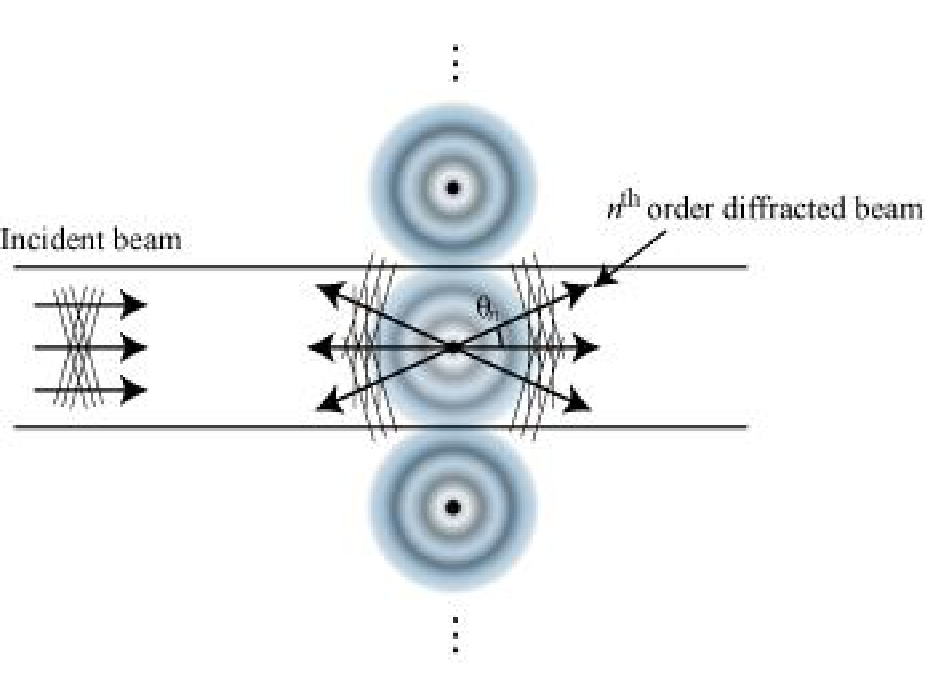
Each order of the diffracted beam will have a different weighting; our object is to cast our Green’s function (18) in a manner that makes these weightings explicit. This formulation is of interest because it is equivalent to determining the transmission and reflection coefficients of our system. Namely, if we send in a mode, we would like to know what modes come out and with what intensities, which is precisely what we shall find by casting our scattering wavefunction as a diffracted beam.

To begin, we note that Bessel functions are regular, and consequently have plane wave expansions. In fact, the well-known integral form of the Bessel function

\displaystyle J_{0}(kr)

\displaystyle=

\displaystyle\frac{1}{2\pi}\int_{0}^{2\pi}e^{i\vec{k}(\theta)\cdot\vec{r}}d\theta

(101)

expresses the Bessel function as an isotropic sum of plane waves emanating in all directions from the origin. We can rewrite (101) in terms of a line integral over $k_{y}$ as

	$\displaystyle J_{0}(kr)$	$\displaystyle=$	$\displaystyle\frac{1}{2\pi}\int_{C}\frac{d(k\sin\theta)}{k\cos\theta}e^{i(k_{x},k_{y})\cdot(x,y)}$		(102)
		$\displaystyle=$	$\displaystyle\frac{1}{2\pi}\int_{C}\frac{dk_{y}}{k_{x}}e^{i(k_{x},k_{y})\cdot(x,y)}$		(103)

where $C$ lies along the real axis, going back and forth within the interval $(-k,k)$ .

We seek an analogous expression for the Hankel function. Since $|k_{y}|$ is always less than $k$ in (103), $k_{x}$ is always real, and the plane waves in (103) do not include evanescent waves. Suppose we modify the right-hand side of (103). By permitting $k_{y}$ to range from $-\infty$ to $\infty$ , we may include contributions from all possible evanescent waves, yielding

\frac{1}{2\pi}\int_{-\infty}^{\infty}\frac{dk_{y}}{k_{x}}e^{i(k_{x},k_{y})\cdot(x,y)}.

(104)

For $|k_{y}|>k,$ the corresponding value of $k_{x}=\pm i\kappa_{x}$ , where $\kappa_{x}\equiv\sqrt{k_{y}^{2}-k^{2}},$ is imaginary. Choosing the positive value makes the evanescent waves die off to the right $(x>0)$ and diverge to the left $(x<0).$ Therefore, with this choice of sign, we may expect (104) to converge only in the right half-plane.

By adding on an evanescent contribution to the Bessel function’s plane wave expansion, we have in fact arrived (up to a constant) at an integral form of the Hankel function, valid in the right half-plane only,

\displaystyle H_{0}^{(1)}(kr)

\displaystyle=

\displaystyle\frac{1}{\pi}\int_{-\infty}^{\infty}\frac{dk_{y}}{k_{x}}e^{i(k_{x},k_{y})\cdot(x,y)}

(105)

where

k_{x}=\left\{\begin{array}[]{ccc}\sqrt{k^{2}-k_{y}^{2}}&&\left|k_{y}\right|\leq k\\ i\sqrt{k_{y}^{2}-k^{2}}&&\left|k_{y}\right|>k.\end{array}\right.

(106)

Eq. (105) is a well-known expansion,Morse and Feshbach 1953 readily obtained by Fourier transforming Green’s equation.

Consider now the sum

G_{p}(\vec{r};d)=-\frac{i}{2}\sum_{n=-\infty}^{\infty}H_{0}(k\left|\vec{r}-(x_{0},nd)\right|)

(107)

which is the Green’s function for a fully periodic array of scatterers at $(x_{0},nd)$ (or equivalently, a periodic wire with walls at $y=0,y=2d$ and a scatterer halfway between). Based on the physical picture of diffraction (Fig. 7), the sum in (107) must be a superposition of plane and evanescent waves at real and complex Bragg angles respectively. We wish to find the weighting on each wave (analogous to the structure factor in X-ray diffraction).

To find the weights, we calculate the expansion explicitly. Using (105) in (107), we find

$\displaystyle G_{p}(\vec{r},\vec{0})$	$\displaystyle=$	$\displaystyle-\frac{i}{2}\sum_{n=-\infty}^{\infty}H_{0}(k\|\vec{r}-\vec{r}_{n}\|)$	(108)
	$\displaystyle=$	$\displaystyle-\frac{i}{2\pi}\sum_{n=-\infty}^{\infty}\int_{-\infty}^{\infty}\frac{dk_{y}}{k_{x}}$	(109)
		$\displaystyle\hskip 36.135pt\times e^{i(k_{x},k_{y})\cdot(x-x_{0},y-nd)}$	(109)
	$\displaystyle=$	$\displaystyle-\frac{i}{2\pi}\int_{-\infty}^{\infty}\frac{dk_{y}}{k_{x}}e^{i(k_{x},k_{y})\cdot(x-x_{0},y)}$	(110)
		$\displaystyle\hskip 36.135pt\times\sum_{n=-\infty}^{\infty}\left(e^{-i(k_{y}d)}\right)^{n}$	(110)
	$\displaystyle=$	$\displaystyle-\frac{i}{d}\int_{-\infty}^{\infty}\frac{dk_{y}}{k_{x}}e^{i(k_{x},k_{y})\cdot(x-x_{0},y)}$	(111)
		$\displaystyle\hskip 36.135pt\times\sum_{m=-\infty}^{\infty}\delta(k_{y}-\frac{2m\pi}{d})$	(111)

where we have used

\sum_{n=-\infty}^{\infty}\left[e^{ik_{y}d}\right]^{n}=2\pi\sum_{n=-\infty}^{\infty}\delta(k_{y}d-2\pi n),

(112)

(similar to stationary phase) to reach the expression (111). One can, more rigorously, reach (111) via the Poisson sum formula.Abramowitz and Stegun 1965; Linton and Martin 2004

Performing the integral in (111) yields the final expression

	$\displaystyle G_{p}(\vec{r},\vec{r}_{m};k,d)$	$\displaystyle=$	$\displaystyle-\frac{i}{d}\sum_{n=-\infty}^{\infty}\frac{1}{k_{x}^{(n)}}e^{ik_{x}^{(n)}\|x-x_{0}\|}$		(113)
			$\displaystyle\hskip 36.135pt\times\cos(k_{y}^{(n)}y)$		(113)

where we use the absolute value signs to extend the Green’s function to converge on $x<x_{0},$ and we define

	$\displaystyle k_{x}^{(n)}$	$\displaystyle=$	$\displaystyle k\cos\theta_{n}$		(114)
	$\displaystyle k_{y}^{(n)}$	$\displaystyle=$	$\displaystyle k\sin\theta_{n}$		(115)

where the $\theta_{n}$ are the Bragg angles

\theta_{n}=\arcsin\frac{2n\pi}{kd}\qquad n\mathrm{\>integer}

(116)

and the complex-valued $\theta_{n}$ are the result of the logarithmic singularity.

The image representation of our wire is not exactly the periodic array of Fig. 7. The images alternate in sign, and in general the scatterer is off-center. We can, however, represent our image array as a sum of two arrays, as in Fig. 8.

One can easily verify that the Green’s function for the wire with point source at $\vec{r}_{0}=(x_{0},y_{0})$ becomes the sum

$\displaystyle G_{w}(\vec{r},\vec{r}_{0})$	$\displaystyle=$	$\displaystyle\frac{1}{2}[G_{p}(\vec{r}-y_{0}\hat{y};2d)$	(117)
		$\displaystyle\hskip 36.135pt-G_{p}(\vec{r}+y_{0}\hat{y};2d)]$	(117)
	$\displaystyle=$	$\displaystyle-i\sum_{n=1}^{\infty}\frac{1}{k_{x}^{(n)}}e^{ik_{x}^{(n)}\|x-x_{0}\|}$	(118)
		$\displaystyle\hskip 36.135pt\times\chi_{n}(y)\chi_{n}(y_{0})$	(118)

where the Bragg angles are modified slightly from the case of the periodic wire, and defined by

\sin\theta_{n}=\frac{n\pi}{kd}.

(119)

The form (118) is identical to (14). We have shown that diffraction translates the method of images into the usual eigenfunction expansion of the Green’s function.

Appendix B Improving convergence of the green’s function

Form (14) of the Green’s function converges slowly also. The reason for the slow convergence is the singularity at the source, which is present but disguised in the evanescent modes. We use the Kummer method for convergence acceleration,Abramowitz and Stegun 1965 which also makes the singularity explicit. Kummer’s method involves adding and subtracting a multiple of the static ( $k=0$ ) Green’s function. We note that [12] obtains similar results, via a slightly different procedure.

The wire Green’s function is

	$\displaystyle G_{w}(\vec{r},\vec{r};k)$	$\displaystyle=$	$\displaystyle-i\sum_{m=1}^{\infty}\frac{1}{k_{x}^{(m)}}\chi_{m}(y)\chi_{m}(y_{0})$		(120)
			$\displaystyle\hskip 36.135pt\times e^{ik_{x}^{(m)}\left\|x-x_{0}\right\|}$		(120)

We wish to consider a more rapidly converging form of the Green’s function:

	$\displaystyle G_{w}(\vec{r},\vec{r}_{0};k)$	$\displaystyle=$	$\displaystyle\left[G_{w}(\vec{r},\vec{r}_{0};k)-\alpha G_{w}(\vec{r},\vec{r}_{0};0)\right]$		(121)
			$\displaystyle\hskip 36.135pt+\alpha G_{w}(\vec{r},\vec{r}_{0};0)$		(121)

where $\alpha$ is a constant which we shall determine. The static Green’s function happens to be the potential which solves Poisson’s equation for a point charge between two grounded, conducting plates,Morse and Feshbach 1953 and we can put it in closed form as follows:

$\displaystyle G_{w}(\vec{r},\vec{r}_{0};0)$	$\displaystyle=$	$\displaystyle-\sum_{m=1}^{\infty}\frac{d}{m\pi}\chi_{m}(y)\chi_{m}(y_{0})e^{-\frac{m\pi}{d}\left\|x-x_{0}\right\|}$	(122)
	$\displaystyle=$	$\displaystyle-\frac{1}{\pi}\sum_{m=1}^{\infty}\frac{d}{m}\times\frac{2}{d}\sin\left(\frac{m\pi y}{d}\right)$	(123)
		$\displaystyle\hskip 18.06749pt\times\sin\left(\frac{m\pi y_{0}}{d}\right)e^{-\frac{m\pi}{d}\left\|x-x_{0}\right\|}$	(123)
	$\displaystyle=$	$\displaystyle\frac{1}{\pi}\sum_{m=1}^{\infty}\frac{1}{m}\left[\cos\left(\frac{m\pi(y+y_{0})}{d}\right)\right.$	(124)
		$\displaystyle\hskip 18.06749pt\left.-\cos\left(\frac{m\pi(y-y_{0})}{d}\right)\right]e^{-\frac{m\pi}{d}\left\|x-x_{0}\right\|}$	(124)
	$\displaystyle=$	$\displaystyle\frac{1}{\pi}\textrm{Re }\sum_{m=1}^{\infty}\frac{1}{m}e^{-\frac{m\pi}{d}\left\|x-x_{0}\right\|}$	(125)
		$\displaystyle\hskip 36.135pt\times\left[e^{\frac{im\pi(y+y_{0})}{d}}-e^{\frac{im\pi(y-y_{0})}{d}}\right]$	(125)
	$\displaystyle=$	$\displaystyle\frac{1}{\pi}\textrm{Re }\sum_{m=1}^{\infty}\left(\frac{Z_{+}^{m}}{m}-\frac{Z_{-}^{m}}{m}\right)$	(126)

where

Z_{\pm}\equiv e^{-\frac{\pi}{d}\left|x-x_{0}\right|}e^{\frac{i\pi(y\pm y_{0})}{d}}.

(127)

Using the identities

\sum_{m=1}^{\infty}\frac{Z^{m}}{m}=-\ln(1-Z)

(128)

and

{\rm Re}\ln Z=\ln|Z|

(129)

we find

$\displaystyle G_{w}(\vec{r},\vec{r}_{0};0)$	$\displaystyle=$	$\displaystyle\frac{1}{\pi}\ln\left\|\frac{1-Z_{-}}{1-Z_{+}}\right\|$	(130)
	$\displaystyle=$	$\displaystyle\frac{1}{2\pi}\ln\left(\left\|\frac{1-Z_{-}}{1-Z_{+}}\right\|^{2}\right)$	(131)
	$\displaystyle=$	$\displaystyle\frac{1}{2\pi}\ln\left\|\frac{e^{\frac{\pi}{d}\left\|x-x_{0}\right\|}-e^{\frac{i\pi}{d}(y-y_{0})}}{e^{\frac{\pi}{d}\left\|x-x_{0}\right\|}-e^{\frac{i\pi}{d}(y+y_{0})}}\right\|^{2}$	(132)
	$\displaystyle=$	$\displaystyle\frac{1}{2\pi}\ln\left[\frac{\left(e^{\frac{\pi}{d}\left\|x-x_{0}\right\|}-e^{\frac{i\pi}{d}(y-y_{0})}\right)}{\left(e^{\frac{\pi}{d}\left\|x-x_{0}\right\|}-e^{\frac{i\pi}{d}(y+y_{0})}\right)}\right.$	(133)
		$\displaystyle\hskip 18.06749pt\left.\times\frac{\left(e^{\frac{\pi}{d}\left\|x-x_{0}\right\|}-e^{-\frac{i\pi}{d}(y-y_{0})}\right)}{\left(e^{\frac{\pi}{d}\left\|x-x_{0}\right\|}-e^{-\frac{i\pi}{d}(y+y_{0})}\right)}\right]$
	$\displaystyle=$	$\displaystyle\frac{1}{2\pi}\ln\frac{\cos\left[\frac{\pi}{d}(y-y_{0})\right]-\cosh\left[\frac{\pi}{d}(x-x_{0})\right]}{\cos\left[\frac{\pi}{d}(y+y_{0})\right]-\cosh\left[\frac{\pi}{d}(x-x_{0})\right]}.$

The singularity of the Green’s function arises from a logarithmic singularity in the Hankel term at the source. Near the scatterer, the contribution from this term becomes

$\displaystyle\lim_{r\rightarrow r_{0}}G_{0}(r,r_{0};k)$	$\displaystyle=$	$\displaystyle-\frac{i}{2}\lim_{\vec{r}\rightarrow\vec{r}_{0}}H_{0}(k\left\|\vec{r}-\vec{r}_{0}\right\|)$	(134)
	$\displaystyle=$	$\displaystyle-\frac{i}{2}+\frac{1}{\pi}\ln\left(\frac{k}{2}\left\|\vec{r}-\vec{r}_{0}\right\|\right)$	(135)
		$\displaystyle\hskip 36.135pt+\frac{1}{\pi}\gamma$	(135)
	$\displaystyle=$	$\displaystyle-\frac{i}{2}+\frac{\gamma-\ln 2}{\pi}$	(136)
		$\displaystyle\hskip 36.135pt+\frac{1}{\pi}\ln\left(k\|r-r_{0}\|\right)$	(136)

where $\gamma$ is the Euler-Mascheroni constant, while from Eq. (133), we find that the limiting behavior of the static Green’s function is (after some algebra)

	$\displaystyle\lim_{\vec{r}\rightarrow\vec{r}_{0}}G_{w}(\vec{r},\vec{r}_{0};0)$	$\displaystyle=$	$\displaystyle-\frac{1}{\pi}\ln\frac{2kd}{\pi}\sin\left(\frac{\pi y_{0}}{d}\right)$		(137)
			$\displaystyle+\frac{1}{\pi}\ln\left(k\|r-r_{0}\|\right).$		(137)

In order to cancel the logarithmic singularity in Green’s function, we thus require that

\alpha=1

(138)

so that

	$\displaystyle\lim_{\vec{r}\rightarrow\vec{r}_{0}}\left[G_{w}(\vec{r},\vec{r}_{0};0)-G_{0}(\vec{r},\vec{r}_{0};k)\right]$	$\displaystyle=$			(139)
			$\displaystyle\hskip-108.405pt-\frac{1}{\pi}\ln\left[\frac{kd}{\pi}\sin\left(\frac{\pi y_{0}}{d}\right)\right]+\frac{i}{2}-\frac{\gamma}{\pi}$		(139)

Our final form for the Green’s function, using (121-138) is

$\displaystyle G_{w}(\vec{r},\vec{r}_{0};k)$	$\displaystyle=$	$\displaystyle\sum_{m=1}^{\infty}\chi_{m}(y)\chi_{m}(y_{0})\left(\frac{1}{ik_{x}^{(m)}}e^{ik_{x}^{(m)}\|x-x_{0}\|}\right.$	(140)
		$\displaystyle\hskip 36.135pt\left.+\frac{d}{m\pi}e^{-\frac{m\pi}{d}\|x-x_{0}\|}\right)$
		$\displaystyle+\frac{1}{2\pi}\ln\frac{\cos\left[\frac{\pi}{d}(y-y_{0})\right]-\cosh\left[\frac{\pi}{d}(x-x_{0})\right]}{\cos\left[\frac{\pi}{d}(y+y_{0})\right]-\cosh\left[\frac{\pi}{d}(x-x_{0})\right]}.$

This expression is of further use in that it allows us to obtain another form of the renormalization constant (23), which we had shown to have the slowly convergent expansion

G_{r}=-\frac{i}{2}\sum_{m=1}^{\infty}(-1)^{m}H_{0}(k|\vec{r}_{m}-\vec{r}_{0}|).

(141)

We can now express $G_{r}$ in an equivalent, but more rapidly convergent expression, suitable for numerical purposes:

$\displaystyle G_{r}$	$\displaystyle=$	$\displaystyle\lim_{\vec{r}\rightarrow\vec{r}_{0}}\left(G_{w}(\vec{r},\vec{r}_{0};k)-G_{0}(\vec{r},\vec{r}_{0};k)\right)$	(142)
	$\displaystyle=$	$\displaystyle\lim_{\vec{r}\rightarrow\vec{r}_{0}}\left[\left(G_{w}(\vec{r},\vec{r}_{0};k)-G_{w}(\vec{r},\vec{r}_{0};0)\right)\right.$	(142)
		$\displaystyle\hskip 18.06749pt\left.+\left(G_{w}(r,r_{0};0)-G_{0}(r,r_{0};k)\right)\right]$	(143)
	$\displaystyle=$	$\displaystyle\sum_{m=1}^{\infty}\left(\frac{1}{ik_{x}^{(m)}}+\frac{d}{m\pi}\right)\chi_{m}^{2}(y_{0})$	(143)
		$\displaystyle\hskip 18.06749pt-\frac{1}{\pi}\ln\left[\frac{kd}{\pi}\sin\left(\frac{\pi y_{0}}{d}\right)\right]+\frac{i}{2}-\frac{\gamma}{\pi}.$	(144)

Mirrored wave	Expression	Wavefunction plotted for $kd=40$ (twelve modes open)
$s$	$\frac{1}{2}\sum_{n=-\infty}^{\infty}(-1)^{n}J_{0}(k\left\|\vec{r}-\vec{r}_{n}\right\|)$
$p_{x}$	$\frac{1}{2}\sum_{n=-\infty}^{\infty}(-1)^{n}J_{1}(k\left\|\vec{r}-\vec{r}_{n}\right\|)\cos\theta$
$d_{xy}$	$\sum_{n=-\infty}^{\infty}J_{2}(k\left\|\vec{r}-\vec{r}_{n}\right\|)\sin 2\theta$
$f_{x^{3}-3xy^{2}}$	$\sum_{n=-\infty}^{\infty}(-1)^{n}J_{3}(k\left\|\vec{r}-\vec{r}_{n}\right\|)\cos 3\theta$
$\vdots$	$\vdots$	$\vdots$