∗ email: schuetz@theory.phy.tu-dresden.de
General error estimate for adiabatic quantum computing
Abstract
Most investigations devoted to the conditions for adiabatic quantum computing are based on the first-order correction . However, it is demonstrated that this first-order correction does not yield a good estimate for the computational error. Therefore, a more general criterion is proposed, which includes higher-order corrections as well and shows that the computational error can be made exponentially small – which facilitates significantly shorter evolution times than the above first-order estimate in certain situations. Based on this criterion and rather general arguments and assumptions, it can be demonstrated that a run-time of order of the inverse minimum energy gap is sufficient and necessary, i.e., . For some examples, these analytical investigations are confirmed by numerical simulations.
pacs
03.67.Lx, 03.67.-a.I Introduction
With the emergence of the first quantum algorithms, it turned out that quantum computers are in principle much better suited to solving certain classes of problems than classical computers. Prominent examples are Shor’s algorithm shor1997 for the factorization of large numbers into their prime factors in polynomial time and Grover’s algorithm grover1997 for searching an unsorted database with items reducing the computational complexity from the classical value to on a quantum computer.
Unfortunately, the actual realization of usual sequential quantum algorithms (where a sequence of quantum gates is applied to some initial quantum state, see, e.g., nielsen2000) goes along with the problem that errors accumulate over many operations and the resulting decoherence tends to destroy the fragile quantum features needed for the computation. Therefore, an alternative scheme has been suggested farhi2000, where the solution to a problem is encoded in the (unknown) ground state of a (known) Hamiltonian. By starting with an initial Hamiltonian with a known ground state and slowly evolving to the final Hamiltonian with the unknown ground state, e.g., , adiabatic quantum computing makes use of the adiabatic theorem which states that a system will remain near its ground state if the evolution is slow enough. Since there is evidence that the ground state is more robust against decoherence childs2001; kaminsky0211152; sarandy2005b, this scheme offers fundamental advantages compared to sequential quantum algorithms.
However, determining the achievable speed-up of adiabatic quantum algorithms (compared to classical methods) for many problems is still a matter of investigation and debate, see, e.g., znidaric2005; farhi0512159; aharonov0405098; sarandy2004; childs2002; das2003; roland2002. For example, it has been argued in aharonov0405098 that all conventional (sequential) quantum algorithms can be realized as adiabatic quantum computation schemes with polynomial overhead via the history interpolation (polynomial equivalence). For an adiabatic version of Grover’s algorithm, a constant velocity implies a linear scaling of the run-time , whereas a suitably adapted time-dependence yields the known quadratic speed-up , cf. das2003; roland2002. Whether adiabatic algorithms of NP complete problems such as 3-SAT can be even more efficient than this quadratic speed-up is still not clear, see, e.g., znidaric2005; farhi0512159.
In this paper, we derive a general error estimate as a function of the run-time (the main measure for the computational complexity of adiabatic quantum algorithms) for very general gap structures and interpolation velocities .
II Adiabatic Expansion
The evolution of a system state subject to a time-dependent Hamiltonian is described by the Schrödinger equation ()
| (1) |
Using the instantaneous energy eigenbasis defined by , the system state can be expanded to yield
| (2) |
Insertion into the Schrödinger equation yields – after some algebra – the evolution equations for the coefficients
| (3) | |||||
with the energy gap and the Berry phase sun1988
| (4) |
If the external time-dependence is slow (adiabatic evolution), the right-hand side of Eq. (3) is small and the solution can be obtained perturbatively. After an integration by parts, the first-order contribution yields
| (5) |
where denotes a pure phase. Consequently, if the local adiabatic condition
| (6) |
is fulfilled for all times, the system approximately stays in its instantaneous eigen (e.g., ground) state throughout the (adiabatic) evolution. This above constraint has frequently been used as a condition for adiabatic quantum computation farhi2000; childs2002. However, since the solution to a problem is encoded in the ground state of the final Hamiltonian in adiabatic quantum computation schemes, it is not really necessary to be in the instantaneous ground state during the dynamics – the essential point is to obtain the desired ground state after the evolution. Since the external time-dependence could realistically be extremely small (or even practically vanish) at the end of the computation , the first-order result (5) does not always provide a good error estimate. Similar to the theory of quantum fields in curved space-times birrell, the difference between the adiabatic and the instantaneous vacuum should not be confused with real excitations (particle creation). Therefore, it is necessary to go beyond the first-order result above and to estimate the higher-order contributions.
III Analytic Continuation
Evidently, the Schrödinger equation is covariant under simultaneous transformations of time and energy, such that the runtime of any adiabatic algorithm can be reduced to constant if the energy of the system is modified accordingly das2003. Here we want to exclude a mixing of these effects and will therefore assume
| (7) |
where is an interpolation function which will be specified below. In practice, the above condition can even be relaxed to the demand that the trace should not vary by orders of magnitude (during ). With suitable initial and final Hamiltonians and , the above condition can be satisfied for all by using the linear interpolation scheme
| (8) |
but other schemes are also possible (see section V). For simplicity, we restrict our considerations in this section to a non-degenerate (instantaneous) ground state and one single first exited state with . (Multiple excited states will be discussed in section V.) Similarly, all energies will be normalized in units of a typical energy scale corresponding to the initial/final gap, i.e., and . We classify the dynamics of via a function
| (9) |
where the function is constrained by the conditions and . Insertion of this ansatz into Eq. (3) yields the exact formal expression for the non-adiabatic corrections to a system starting in the ground state, i. e., with one obtains after time
| (10) | |||||
with the matrix elements which simplify in the case (8) of linear interpolation to . The advantage of the form in Eqs. (9) and (10) lies in the fact that different time-dependences and hence different choices for solely modify the exponent.
We assume that all involved functions can be analytically continued into the complex -plane and are well-behaved near the real -axis. Given this assumption, we may estimate the integral in Eq. (10) via deforming the integration contour into the lower complex half-plane (to obtain a negative exponent – which is the usual procedure in such estimates) until we hit a saddle point, a singularity, or a branch cut, see Fig. 1. Deforming the integration contour into the upper complex half-plane would of course not change the result, but there the integrand is exponentially large and strongly oscillating such that the integral is hard to estimate. Since the gap usually has a pronounced minimum at , the first obstacle we encounter well-behaved will be a singularity at close to the real axis, i.e., and , where .

Let us first consider a constant function : Assuming (i.e., slow evolution), the exponent in Eq. (10) acquires a large negative real part for and thus the absolute value of the integrand decays rapidly if we depart from the real -axis in the lower complex half-plane. Imposing the even stronger constraint , the decay of the exponent dominates all the other -dependences [, , and ] since their typical (minimum well-behaved) scale of variation is . In view of the complex continuation of Eq. (3), the same applies to the amplitude . As a result, the above integral (10) will be exponentially suppressed if holds, which (as one would expect) implies a large evolution time via the side condition .
The general situation with varying can be treated in complete analogy – the integral in Eq. (10) is suppressed provided that the condition
| (11) |
holds for all singularities (and saddle points etc.) in the lower complex half-plane (which determine the deformation of the integration contour). Together with
| (12) |
this determines an upper bound for the necessary runtime of the quantum adiabatic algorithm.
Note that the constraint derived from is not necessarily equivalent to , which one would naively deduce from Eq. (6).
IV Evolution time
The general criterion in Eq. (11) can now be used to estimate the necessary run-time via Eq. (12). Typically, the inverse energy gap is strongly peaked (along the real axis) around with a width well-behaved of order . Therefore, assuming to be roughly constant across the peak and respecting , yields the following estimate of the integral in Eq. (12)
| (13) |
where denotes the minimum energy gap. Note that this estimate is only valid for one (or a few) relevant excited state(s) – multiple excited states will be discussed in section V.
Intuitively, the same order of magnitude estimate for the evolution time can also be derived from the local adiabatic condition (6): Inverting this condition, we find the relationship
| (14) |
Assuming that does not oscillate strongly, e.g., that the ground state of travels on a reasonably direct path from the initial to the final state, we can make the following estimate
| (15) |
Now we may exploit the advantage of the representation in Eq. (10), which is valid for general dynamics corresponding to different functions and hence for arbitrary evolution times . In the limit of very fast evolution (which implies ), we have large excitations and thus the remaining integral in the above equation can be estimated via inserting this limit into Eq. (10):
| (16) |
By comparing Eqs. (16) and (14), we again obtain the estimate (13). Note that the quantities and appearing in the integrals in Eqs. (14-16) do not depend on the dynamics which allows us to perform the integration independently of .
IV.1 Gap Structure
Let us illustrate the above considerations by means of the rather general ansatz for the behavior of the gap
| (17) |
with the minimal gap at , , and . An avoided level crossing in an effectively two-dimensional subspace corresponds to . This is the typical situation if the commutator of the initial and the final Hamiltonian is small, since, in this case, the two operators can almost be diagonalized independently and thus the energy levels are are nearly straight lines except at the avoided level crossing(s), where becomes important. In the continuum limit, such an (Landau-Zener type) avoided level crossing corresponds to a second-order quantum phase transition. The finite-size analogue of a third-order phase transition corresponds to (and accordingly for even higher orders), which may occur if is not small or if the interpolation is not linear, i.e., .
The inverse gap has singularities around at , compare Fig. 1. The total running time for different choices of satisfying the criterion (11) can be obtained from Eq. (12). Here, the exponent determines the scaling of the interpolation dynamics, whereas the coefficient is adapted such that , cf. Eqs. (9) and (12).
For one easily shows that satisfies the criterion (11) with the evolution time obeying . If is smaller, the necessary evolution time will be larger. In Table 1, the scaling of the run-time (for two examples of the gap structure) is derived for three cases:
- a)
constant velocity , i.e., ,
- b)
constant function , i.e., , and
- c)
the local adiabatic evolution with , i.e., , investigated in roland2002.
IV.2 Grover’s Algorithm
In the frequently studied adiabatic realization of Grover’s algorithm (see, e.g., childs2002; das2003; roland2002) the initial Hamiltonian reads with the initial superposition state , and the final Hamiltonian is given by , where denotes the marked state. In this case, the commutator is very small and one obtains for the time-dependent gap roland2002
| (18) | |||||
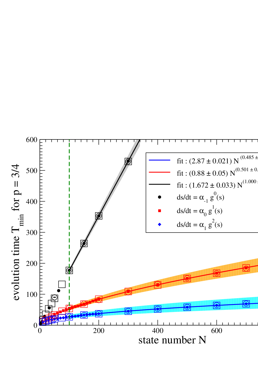
Comparing with Eq. (17), we identify and (the pre-factor does not affect the scaling behavior). Consequently, our analytical estimate implies for , for , and for .
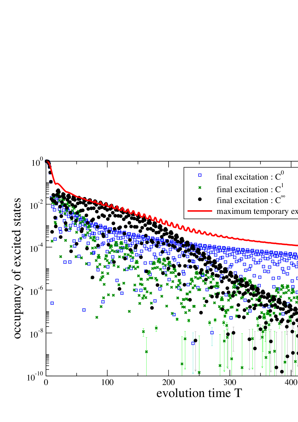
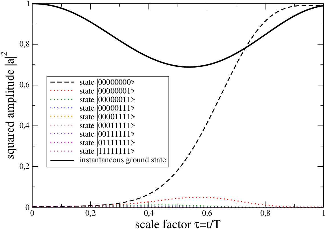
We have solved the Schrödinger equation numerically by using a fourth order Runge-Kutta integration scheme with an adaptive step-size press1994. By restarting the code with different until agreement with desired fidelity was sufficient, we could confirm these runtime scaling predictions numerically, see Fig. 2. The dependence of the final error on the run-time for fixed and constant is depicted in Fig. 3, where the exponential decay becomes evident. The evolution of the instantaneous ground-state occupation is plotted in Fig. 4 for the three different dynamics.


V Further generalizations
V.1 Adiabatic Switching
From an experimental point of view, the time-dependence of the Hamiltonian will most certainly vanish asymptotically or at least be negligible – which automatically implies . Furthermore, realistic Hamiltonians should be described by -interpolations (Natura non facit saltus).
By using a -test function which was matched at and to the usual dynamics (compare dotted lines in figure 4 bottom panel), we have implemented an interpolation scheme with such an adiabatic switching on and off . For the investigated adiabatic implementation of the Grover search routine, this scheme does not affect the final result considerably. The reason for this robustness lies in the fact that the matrix element is peaked around and as well as are small enough already without the adiabatic switching on and off. Therefore, one can expect the dominant non-adiabatic corrections to arise from the behavior around the minimum gap, which was unaffected by the test function. This is also confirmed by the scaling of the runtime versus the system size, compare the hollow circle symbols in figure 2, which is basically unchanged.
However, the situation is completely different for the example considered in section V.3 below. There, the exponential suppression of the final error as a function of the run-time requires a smooth -interpolation – with other dynamics such as (just continuous) or (differentiable once), the final error is merely polynomially small, cf. figure 5.
V.2 Nonlinear Interpolation
Although we have chosen a linear interpolation scheme (8) in order to satisfy the trace constraint (7), the presented analysis can be generalized easily to more general non-linear interpolations. [Note that, linear refers to the straight connection line between initial and final Hamiltonian in equation (8) and should not be confused with the different velocities at which this line is traversed.] The argumentation based on the analytic continuation works in the same way provided that the functional dependence does not involve extremely large or small numbers.
As an illustrative example, we consider the Grover search with the same initial and final Hamiltonians but a quadratic interpolation scheme
| (19) | |||||
where denotes the anti-commutator. The identity operator has been added in order to ensure , cf. equation (7). Although the spectrum of this non-linear interpolation is slightly distorted compared to the linear one, the fundamental gap is the same as in equation (18), and hence same interpolation functions , applied to the above Hamiltonian, should reproduce the aforementioned scaling predictions. This is confirmed by the numerical analysis of the scaling behavior – the results of the non-linear interpolation are basically indistinguishable from those of the previous example (linear interpolation), compare the hollow box symbols in figure 2.
V.3 Degeneracy
So far, we have restricted our considerations to the instantaneous ground state and a single first excited state. Let us now consider a very simple example (see also farhi0512159) in which there is still a unique ground state, but many degenerate first excited states: In terms of single-qubit Pauli matrices and , the -qubit Hamiltonian reads
| (20) |
where we have used a linear interpolation (8) for simplicity. In this example, the Hamiltonian can be decomposed completely into independent and equal single-qubit contributions and hence the time-evolution operator factorizes, i.e., it is sufficient to solve the dynamics of a single qubit. Furthermore, the Hamiltonian is invariant under any permutation of the qubits. The instantaneous ground states for all values of are symmetric under this permutation group and hence unique, but the first excited states are not – leading to a -fold degeneracy (i.e., there are equivalent first excited states). Hence, the fundamental gap between the ground state and each one of these first excited states is the same as for one qubit and thus independent of the number of qubits .
In some sense, this simple example represents a limiting case opposite to Grover’s algorithm: The energy gap and the matrix elements do not scale with the number of qubits and the are neither small initially nor finally. Instead, the scaling with system size manifests itself in the -fold degeneracy of the first excited states. As a result of the -independent gap structure, the adiabatic switching is crucial for achieving the exponential suppression of the final error. Figure 5 displays the final error probabilities for a smooth -interpolation and for and -interpolations for comparison. These numerical simulations confirm that the falloff is exponential in the -case but merely polynomial for and .
Another interesting point of this simple example is the difference between the intermediate and the final occupation of the ground state, see figures 6 and 5. According to the first-order result in Eq. (5) and the aforementioned factorization of the time-evolution operator, the intermediate excitation probability scales as
| (21) |
since the gap is independent of . On the other hand, the final error probability (assuming a -interpolation) is exponentially suppressed
| (22) |
and hence the two error probabilities can be vastly different , cf. figure 6. In fact, by increasing the number of qubits, the occupancy of the instantaneous ground state can be made arbitrarily small. Moreover, the run-time condition derived from the first-order result in Eqs. (5) and (21)
| (23) |
yields a scaling which is far too pessimistic compared with the correct final error probability assuming a -interpolation
| (24) |
Note that non-smooth interpolations (e.g., or ) would also yield a polynomial scaling similar to Eq. (23). On the other hand, the scaling behavior in Eqs. (22) and (24) is just what one would obtain by immersing the system in Eq. (20) into a zero-temperature environment and letting it decay towards its ground state. Therefore, using non-smooth interpolations (e.g., or ) or naively demanding the first-order estimate in Eq. (5), the adiabatic algorithm would be even slower than this simple decay mechanism.
VI Summary
The instantaneous occupation of the first excited state during the adiabatic evolution in Eqs. (5) and (6) does not provide a good error estimate. Instead, a better estimate is given by the remaining real excitations after the dynamics. For the example plotted in Fig. 4, the instantaneous excitation probability exceeds 10% at intermediate times – whereas the final value is 1%. This is even more drastic for the example in section V.3, see figure 6, where the two values and hence the inferred run-times can differ by orders of magnitude.
Moreover, the final error can be made extremely – in fact, with , exponentially – small
| (25) |
cf. Fig. 3. For the Grover example, the last term was dominant, whereas in the general case the smallness of the first two terms can be ensured by using smoothed -interpolations, i.e., adiabatic switching – which is a more realistic ansatz anyway.
Based on general arguments, the optimal run-time (in the absence of degeneracy, cf. section V.3) scales as contrary to what one might expect from the Landau-Zener landau-zener formula (with ). In view of the fact that the minimum energy gap is a measure of the coupling between the known initial state and the unknown final state, this result is very natural.
For the Grover algorithm, it is known that the -scaling is optimal roland2002. This optimal scaling can already be achieved with interpolation functions which vary less strongly (e.g., ) than demanded by locally roland2002 adiabatic evolution () – and hence should be easier to realize experimentally.
Unfortunately, a constant velocity with does not produce the optimal result in general. The Grover example has the advantage that the spectrum can be determined analytically, which is for example not the case for the more involved satisfiability problems farhi2000. Therefore, some knowledge of the spectral properties is necessary for achieving the optimal result also in the general case of adiabatic quantum computing. For systems with an analytically unknown gap structure, some knowledge about the spectrum can be obtained by extrapolating the scaling behavior of small systems.
A related interesting point is the impact of the gap structure (corresponding to or order transition etc.) in Eq. (17). The derived constraint for the velocity at the transition is only for -order transitions equivalent to , which one would naively deduce from Eq. (6).
Note that the improvement compared with the conventional runtime estimate is merely polynomial (same complexity class). Though this is not as impressive as an exponential speedup, in practice a polynomial improvement may be useful. For time-dependent Hamiltonians where the inverse of the minimum gap scales exponentially with the size of the problem, we would still expect an exponential scaling of the runtime required to reach a fixed fidelity (as in section IV.2). On the other hand, the exponential suppression of the final error in Eq. (25) may become important in certain cases such as in the presence of degeneracy and may well yield an exponential speedup in comparison with the conventional estimate, see section V.3.
In some sense, the two examples in sections IV.2 and V.3 represent two simple extremal examples for adiabatic quantum computing regarding the scaling of the gap and the degeneracy. For more complicated situations such as satisfiability problems farhi2000, both properties have to be taken into account simultaneously.
Acknowledgments
R. S. acknowledges fruitful discussions during the workshop ”Low dimensional Systems in Quantum Optics” at the CIC in Cuernavaca (Mexico), which was supported by the Humboldt foundation. G. S. acknowledges fruitful discussions with M. Tiersch. This work was supported by the Emmy Noether Programme of the German Research Foundation (DFG) under grant No. SCHU 1557/1-1/2.
Note added
Recently, two of the main results of this article, i.e., the optimal run-time scaling and the faster-than-polynomial decrease of the final error , have been demonstrated rigorously for a class of Hamiltonians using methods of spectral analysis jansen0603175.
References
- (1) P. W. Shor, SIAM J. Comp. 26, 1484 (1997).
- (2) L. K. Grover, Phys. Rev. Lett. 79, 325 (1997).
- (3) M. A. Nielsen and I. L. Chuang, Quantum Computation and Quantum Information (Cambridge University Press, Cambridge, England, 2000).
- (4) E. Farhi et al., Science 292, 472 (2001).
- (5) A. M. Childs, E. Farhi, and J. Preskill, Phys. Rev. A 65, 012322 (2001).
- (6) W. M. Kaminsky and S. Lloyd, in Quantum Computing and Quantum Bits in Mesoscopic Systems by A. Leggett et al. (eds.) (Kluwer Academic, 2003); pre-print: quant-ph/0211152.
- (7) M. S. Sarandy and D. A. Lidar, Phys. Rev. Lett. 95, 250503 (2005).
- (8) M. Z̆nidaric̆, Phys. Rev. A 71, 062305 (2005); M. Z̆nidaric̆ and M. Horvat, pre-print: quant-ph/0509162.
- (9) E. Farhi et al., pre-print: quant-ph/0512159.
- (10) D. Aharonov et al., 45th Annual IEEE Symposium on Foundations of Computer Science, 42-51, (2004); pre-print: quant-ph/0405098.
- (11) M. S. Sarandy, L.-A. Wu, and D. A. Lidar, Quant. Inf. Proc. 3, 331 (2004).
- (12) A. M. Childs et al., Quant. Inf. Comp. 2, 181 (2002).
- (13) S. Das, R. Kobes, and G. Kunstatter, J. Phys. A 36, 2839 (2003).
- (14) J. Roland and N. J. Cerf, Phys. Rev. A 65, 042308 (2002).
- (15) C.-P. Sun, J. Phys. A 21, 1595 (1988).
- (16) N. D. Birrell and P. C. W. Davies, Quantum Fields in Curved Space, (Cambridge University Press, Cambridge, England 1982).
- (17) Since the functions , , and are supposed to be well-behaved near the real -axis, there are no small (or large) numbers in the problem apart from those generated by the minimum of the gap . Thus the significant changes of the eigenvectors are also localized around this minimum. In the complex plane, this minimum along the real axis becomes a saddle point. For analytic functions, the characteristic length scale of variation must be the same along the real axis and into the complex plane (of order ) and is determined by the lowest non-trivial Taylor coefficient at that point.
- (18) W. H. Press et al., Numerical recipes in C (Cambridge University Press, Cambridge, England 1994).
- (19) C. E. Zener, Proc. R. Soc. London, Ser. A 137, 696 (1932); L. D. Landau and E. M. Lifshitz, Quantum Mechanics (Pergamon Press, London, 1958).
- (20) S. Jansen, M. B. Ruskai, and R. Seiler, pre-print: quant-ph/0603175.