Non-Markovian quantum dynamics: Correlated projection superoperators and Hilbert space averaging
Abstract
The time-convolutionless (TCL) projection operator technique allows a systematic analysis of the non-Markovian quantum dynamics of open systems. We introduce a class of projection superoperators which project the states of the total system onto certain correlated system-environment states. It is shown that the application of the TCL technique to this class of correlated superoperators enables the non-perturbative treatment of the dynamics of system-environment models for which the standard approach fails in any finite order of the coupling strength. We demonstrate further that the correlated superoperators correspond to the idea of a best guess of conditional quantum expectations which is determined by a suitable Hilbert space average. The general approach is illustrated by means of the model of a spin which interacts through randomly distributed couplings with a finite reservoir consisting of two energy bands. Extensive numerical simulations of the full Schrödinger equation of the model reveal the power and efficiency of the method.
pacs
03.65.Yz, 05.70.Ln, 05.30.-dI Introduction
Realistic quantum mechanical systems are influenced through the coupling to an environment which contains a large number of mostly uncontrollable degrees of freedom. The unavoidable interaction of an open quantum systems with its environment gives rise to the mechanisms of damping and dissipation, and to a strong and often rapid loss of quantum coherence. Applications of the theory of open quantum systems TheWork are found in almost all areas of physics, ranging from quantum optics WallsMilburn to condensed matter physics Weiss and chemical physics Pechukas, from quantum information Nielsen to spintronics Loss. Moreover, the theory of open quantum systems provides the foundations of quantum measurement theory Braginsky, decoherence Giulini and the emergence of thermodynamic behavior GEMMER.
In a microscopic approach one regards the total system, which is composed of the open system and its environment , as a closed quantum system following a Hamiltonian time evolution. One of the central goals of the theoretical treatment is then the analysis of the dynamical behavior of the populations and coherences which are given by the elements of the reduced density matrix . Here, denotes the density matrix of the composite system and the partial trace taken over the environment.
In the Markovian regime a complete mathematical theory is available which is based on the concepts of completely positive quantum dynamical semigroups and the corresponding Markovian master equations in Lindblad form GORINI1; GORINI2; LINDBLAD; SPOHN. However, if the physical conditions underlying the Markov approximation are violated one has to cope with strong non-perturbative and memory effects and the theoretical and mathematical treatment of the reduced system dynamics is typically much more involved.
A systematic approach to non-Markovian dynamics is provided by the projection operator techniques NAKAJIMA; ZWANZIG which are extensively used in nonequilibrium thermodynamics and statistical mechanics GRABERT; KUBO. The key concept of these techniques consists in the introduction of a certain projection superoperator which acts on the operators of the state space of the total system. The superoperator formalizes the idea of the elimination of degrees of freedom from the complete description of the states of the total system. Thus, if is the density matrix of the composite system, the projection serves to represent a simplified effective description through a reduced set of variables. For this reason, the projection is called the relevant part of the total density matrix, while the complementary projection is referred to as irrelevant part.
With the help of the projection operator techniques one derives closed equations of motion for the relevant part from which one obtains approximate master equations by means of a systematic perturbation expansion with respect to the system-environment coupling. We shall concentrate in this paper on a specific variant of the technique which is known as the time-convolutionless (TCL) projection operator method SHIBATA1; SHIBATA2; SHIBATA3; SHIBATA4; ROYER. The advantage of this formulation is that it leads to dynamic equations for which are local in time and involve an explicitly time-dependent generator. A general account of projection operator methods and, in particular, of the TCL approach and its applications may be found in Ref. TheWork.
In the standard approach to the dynamics of open systems one chooses a projection superoperator which is defined by the expression , where is some fixed environmental state. This superoperator projects the total state onto an un-correlated tensor product state. Since is considered as fixed, it implies that the elements of the reduced density matrix represent the relevant variables used for an effective description of the reduced system dynamics. This ansatz for the projection superoperator is widely used in studies of open quantum systems. It has been used to derive Markovian and non-Markovian quantum master equations for many applications (see, e. g., CHANG; DESPOSITO; ANNPHYS; ATOM-LASER; BKP). Moreover, non-Markovian generalized master equations for the reduced density matrix have been developed on the basis of phenomenological considerations LIDAR.
The paradigm of these and many other approaches is the usage of the reduced density matrix as dynamical variable for which appropriate (exact or approximate) dynamic equations are to be developed. However, it is important to realize that the projection operator techniques are much more general and flexible, and that they offer many further possibilities for the construction of suitable projection superoperators. The only formal condition which must be satisfied in order to apply the techniques is that is a map which operates on the total state space and has the property of a projection operator, i. e., . This is a very general condition which can be fulfilled in many different ways.
We mention two examples: In the analysis of classical stochastic processes one considers a projection of the form which takes any stochastic process to its average SHIBATA1. With this choice the TCL technique leads to a cumulant expansion of the dynamic equation for the average KUBO63; ROYER72; KAMPEN1; KAMPEN2. In nonequilibrium thermodynamics a further projection of the form is often introduced which maps any density matrix to its diagonal part in a suitably chosen basis, yielding the famous Pauli master equation in lowest order of the TCL expansion KUBO.
In the present paper we shall construct a class of projection superoperators which enable the non-perturbative treatment of highly non-Markovian processes in open quantum systems. These superoperators project the state of the total system onto a correlated system-environment state, i. e., onto a state which contains statistical correlations between certain system and environment states. Thus, we give up the paradigm of using the reduced density matrix as the dynamical variable, and enlarge the set of relevant variables to account for statistical correlations which are responsible for strong non-Markovian effects. The idea of introducing additional variables has been realized in different ways and used in various contexts GASPARD; GARRAWAY1; GARRAWAY2; IMAMOGLU; GQT; BUDINI. Here, we implement this idea directly in the definition of a projection superoperator and connect it with the method of the TCL technique. This connection enables us to determine higher order corrections in a systematic way and, hence, to assess the quality of the approximations obtained.
Recently, an entirely different approach has been suggested, the Hilbert space average method (HAM) GEMMER; Gemmer01. This method employs the concept of a best guess for conditional quantum expectation values. It is based on the determination of a conditional Hilbert space average. The method provides us with a systematic principle to estimate quantum expectation values conditioned on prescribed values for the expectations of a given set of operators on the total state space. HAM can be used to construct effective equations of motion for the given set of operators and, hence, yields an alternative approach to non-Markovian quantum dynamics. It will be shown here that the method of the Hilbert space average and the projection operator techniques which are based on the class of correlated projection superoperators are closely related. In fact, we are going to demonstrate that HAM represents the lowest order of the TCL expansion corresponding to this class of superoperators.
The application and the efficiency of our approach will be illustrated and discussed here by means of a specific system-reservoir model. The model consists of a spin which interacts with two environmental energy bands through a set of random couplings Gemmer2005; Gemmer2005a. This model exhibits an unexpected feature. Namely, it turns out that the usual Born-Markov approximation fails for this model, although the standard Markov condition is satisfied, i. e., although the width of the environmental two-point correlation function is small compared to the relaxation time. By contrast, it will be demonstrated by means of a comparison with the numerical solution of the full Schrödinger equation of the model that the TCL expansion using the correlated projection superoperator yields accurate results already in lowest order of the perturbation expansion.
The paper is organized as follows. The class of correlated projections will be introduced in Sec. II. This section also contains a brief general account of the projection operator techniques, and introduces the basic dynamic equations as well as the perturbation expansion of the master equations for the relevant variables. The principles and equations of the Hilbert space averaging method are outlined in Sec. III, where we will also describe the connection between the principles of HAM and the structure of the correlated projection superoperators. Sec. IV contains the application of the general concepts developed here to a specific system-reservoir model. We shall discuss in detail the origin of the failure of the Born-Markov approximation, and show that and why the new projection superoperators yield an efficient and accurate approximation of the dynamics. Finally, we draw our conclusions in Sec. V.
II Projection operator techniques
II.1 Projection superoperators
We consider an open quantum system with state space which is coupled to an environment with state space . The Hilbert space of states of the composite system is given by the tensor product . We assume that the dynamics of the total density matrix of the composite system is governed by some Hamiltonian of the form , where generates the free time evolution of the system and of the environment, and describes the system-environment coupling. We work in the interaction representation and write the von Neumann equation of the combined system as
| (1) |
where is the Hamiltonian in the interaction picture, and denotes the corresponding Liouville superoperator.
The projection operator techniques are based on the introduction of a projection superoperator . This is a linear map
| (2) |
which takes any operator on the total state space to an operator on , and which has the property of a projection operator:
| (3) |
Given a map with this property one employs the projection operator techniques to derive from the von Neumann equation (1) for the total density matrix exact and closed equations of motion for its projection (see Sec. II.2). The basic idea underlying this approach is the following. With an appropriate choice for the projection superoperator one intends to obtain a description of the dynamics of system states which is much simpler and much more efficient than the description by means of the full density matrix . Thus, the map expresses the transition from the full representation in terms of the total density matrix to a simplified, effective description through a reduced set of dynamical variables defined by the structure of the projection .
Equation (3) is our first basic condition. It is this condition which allows the formal application of the projection operator techniques to open quantum systems. The ultimate goal is to determine form the equations of motion for the dynamics of the density matrix of the reduced open quantum system. To this end, we need one further condition. Namely, whatever the form of the projection superoperator is, we demand that contains the complete information required to reconstruct . We therefore impose the second basic condition:
| (4) |
The first equation is just the definition of the reduced density matrix which is obtained by taking the partial trace over the environment. The second equation states that, in order to determine , we do not really need the full density matrix of the total system, but only its projection . Hence, the reduced density matrix is found by taking the environmental trace of the equations of motion for .
Within the standard approach to the dynamics of open systems using projection operator techniques one defines a projection superoperator of the form:
| (5) |
where is some fixed environmental density matrix referred to as the reference state. This superoperator clearly satisfies our basic conditions (3) and (4). By use of this the total state of the system is represented by means of the tensor product state . Regarding the reference state as fixed, one uses the reduced density matrix as the dynamical variable. Applying the projection operator technique one then finds a master equation for the reduced density matrix whose coefficients are given by certain multitime correlation functions defined by averages with respect to the reference state . In particular, the master equation obtained in second order of the coupling yields the Born approximation of the dynamics which involves certain two-time environmental correlation functions.
Our new class of correlated projection superoperators is obtained as follows. We take any orthogonal decomposition of the unit operator on the state space of the environment, i. e., a collection of projection operators on which satisfy
| (6) |
Then we can define a linear map by means of
| (7) |
where . It is again easy to verify that this superoperator fulfills the requirements (3) and (4). By contrast to the standard projection (5) which uses a representation by a tensor product state, the new projection (7) employs a set of un-normalized density matrices
| (8) |
in order to describe the states of the composite system. The set of the density matrices therefore represents the dynamical variables defined by the projection superoperator (7). Applying the projection operator technique one is then led to a coupled system of equations of motion for the , from which one obtains the reduced density matrix itself by means of the relation (4):
| (9) |
In the theory of entanglement (see, e. g., Ref. ALBER) a state of the form given by Eq. (7) is called separable or classically correlated WERNER. The approach based on a projection of this form thus tries to approximate the total system’s state through a classically correlated but non-factorizing state. Of course, one can also construct projection superoperators which lead to non-separable (entangled) states . The examples discussed below belong to the classes of projection operators defined by Eqs. (5) and (7).
II.2 Equations of motion
Basically, there are two variants of the projection operator technique. The first one is the prominent Nakajima-Zwanzig method NAKAJIMA; ZWANZIG. It leads to a first-order integro-differential equation for which contains a time integration over the past system history involving a certain memory kernel. The second variant is known as time-convolutionless (TCL) projection operator technique SHIBATA1; SHIBATA2 which yields a time-local equation of motion for . We shall use this second variant of the projection operator technique in the present paper. Its advantage is that in any order of the coupling one only has to solve a first-order differential equation which is local in time. It should be emphasized, however, that the general considerations developed here may also be applied to the Nakajima-Zwanzig projection operator technique.
The TCL projection operator method leads to an equation of motion for the projection which is of the general form:
| (10) |
This is an exact inhomogeneous linear differential equation of first order. Both the TCL generator of the linear part and the inhomogeneity are explicitly time-dependent superoperators.
The inhomogeneous part of Eq. (10) is determined by the projection of the initial state, where is the projection superoperator complementary to , and denotes the unit map. We observe that the inhomogeneous term vanishes if the initial state satisfies the relation , i. e., if
| (11) |
Obviously, this relation simplifies the equation of motion (10). In the case of the standard projection (5) it implies that is an un-correlated tensor product state, i. e. . In the case of the projection (7), however, Eq. (11) merely implies that the initial state is of the correlated form given by the structure of the projection superoperator (7).
In general, the TCL generator and the inhomogeneity are extremely complicated objects, and the exact solution of Eq. (10) is as difficult as the solution of the full von Neumann equation for the total system. However, Eq. (10) can be used as a starting point of a systematic perturbation expansion with respect to the strength of the interaction Hamiltonian . With the help of the TCL technique one derives a closed expression for the corresponding expansion of the TCL generator:
| (12) |
The -th-order contribution is given by
| (13) | |||||
The quantities
are known as ordered cumulants KUBO63; ROYER72; KAMPEN1; KAMPEN2 and are defined by the following rules: (1) Write a string of the form with factors of in between two ’s. (2) Insert an arbitrary number of factors between the ’s such that at least one stands between two successive ’s. The resulting expression is multiplied by a factor and all ’s are furnished with a time argument: The first time argument is always . The remaining ’s carry any permutation of the time arguments with the only restriction that the time arguments in between two successive ’s must be ordered chronologically. In the above expression we thus have , , etc. (3) Finally, the ordered cumulant is obtained by a summation over all possible insertions of factors and over all allowed distributions of the time arguments.
In many physical applications it may be assumed that the relations
| (14) |
hold, which means that any string containing an odd number of ’s between successive factors of vanishes. Following the above rules one then finds that all odd-order contributions vanish, while the second and the fourth-order terms take the form:
| (15) |
and
| (16) | |||||
The performance of the formal expansion outlined above strongly depends, of course, on the choice of the projection superoperator . In other words, the quality of the approximation obtained by truncating the expansion at a given order crucially depends on the structure of the chosen projection. It is important to note that the technique yields an expansion of a certain system of equations of motion, and not of the reduced system’s density matrix itself. Taking different projection superoperators one uses entirely different sets of dynamical variables which obey completely different equations of motion. Hence, changing the projection superoperator amounts to changing the set of dynamical variables and the whole structure of the equations of motion, and to a non-perturbative re-organization of the expansion. It may even happen that the solution of the equations of motion in a given order for one particular projection represents the solution to all orders for another projection. This point will be illustrated in Sec. IV by means of a specific system-reservoir model.
III Hilbert space averaging approach to the reduced dynamics
III.1 The Hilbert space average method
The Hilbert space average method (HAM) is in essence a technique to produce guesses for the values of quantities defined as functions of a wavefunction if itself is not known in full detail, only some features of it. In particular it produces a guess for the expectation value if the only information about is a set of different expectation values . Such a statement naturally has to be a guess since there are in general many different that are in accord with the given set of but produce possibly different values for . The question now is whether the distribution of ’s produced by the respective set of ’s is broad or whether almost all those ’s yield ’s that are approximately equal. It turns out that if the spectral width of is not too large and is high-dimensional almost all individual yield an expectation value close to the mean of the distribution of ’s. In spite of this being crucial for the following we refer the reader to GEMMER for details. To find that mean one has to average with respect to the ’s. We call this a Hilbert space average and denote it as
| (17) |
This expression stands for the average of over all that feature but are uniformly distributed otherwise. Uniformly distributed means invariant with respect to all unitary transformations that leave unchanged. One may rewrite (17) as
| (18) |
How is to be computed? Any unitary transformation that leaves invariant has to leave invariant, i. e.:
| (19) |
This, however, can only be fulfilled if and this leads to the general form
| (20) |
(In principal there could be addends of the form, e. g., , etc., but since all we are going to consider below together with zero form a group, those addends are already contained in the above sum.)
Furthermore one of course has the following conditions:
| (21) |
One thus obtains
| (22) |
from which the may be determined. Thus, the construction of a given Hilbert space average is defined with the help of Eqs. (22), (20), and (18). According to this scheme “best guesses” for certain expectation values will be produced below. The explanation of HAM in full detail is beyond the scope of this text and can be found in Gemmer2003; GEMMER.
III.2 HAM, projection operators and dynamics
In the following we explain how HAM can be used to produce the reduced dynamics of a quantum system coupled to some environment, just like the techniques described in Sect. II. Consider the full system’s pure state at some time , . Let be a time evolution operator describing the evolution of the system for a short time, i. e., . This allows for the computation of a set of observables at time :
| (23) |
Now assume that rather than itself only the set of expectation values is known. The application of HAM produces a guess for the based on the :
| (24) |
(Note that here the appear rather than the because those are not actually realized states but denote the set of states over which the Hilbert space average has to be taken.) Iterating this scheme, i. e., taking the for the of the next step allows for the stepwise computation of the evolution of the ’s. If the set of the is chosen such that it determines the local state of the considered quantum system completely this technique produces the local reduced dynamics. The result is of course just like HAM itself only a best guess, but for appropriate systems this guess can be rather accurate.
Here, the ’s are chosen specifically as operators corresponding to elements of the reduced density matrix of the considered system and the occupation probability of “energy bands” of the environment:
| (25) |
where are energy eigenstates of the considered system and is as described in Sect. II.1 a projector, projecting out the energy eigenstates of the environment belonging to an interval around some mean band energy labelled by the index . Let , then one gets for the elements of the reduced density matrix:
| (26) |
Thus, the above defined set of expectation values determines the reduced state of the system completely. The set of states which belong to the Hilbert space average defined by the [in the sense of Eq. (18)] is, following the scheme described in Sect. III.1, found to be
| (27) |
(This turns out to be the same state one would have gotten from minimizing the purity under the subsidiary condition set by the given expectation values .) A comparison with the considerations of Sec. II.1 reveals that has exactly the form produced by the application of the projection superoperator [see Eq. (7)]. Exploiting Eqs. (17), (18), and (27) one can write a specific form of Eq. (24) for this case:
| (28) | |||||
Working in the interaction picture the dynamics of the full system is controlled by the interaction . The time evolution is generated by the corresponding Dyson series. Thus, assuming weak interactions Eq. (28) may be evaluated to second order in the interaction strength using an appropriately truncated Dyson series for . This yields after extensive but rather straightforward calculations for the expectation values corresponding to diagonal elements:
| (29) | |||||
and for the expectation values corresponding to off-diagonal elements:
| (30) | |||||
where
| (31) | |||||
Those ’s are essentially integrals over the same environmental temporal correlation functions that appear in the memory kernels of standard projection operator techniques. But here they explicitly correspond to transitions between different energy subspaces of the environment. (In Eqs. (29) and (30) we assumed that correlation functions vanish unless they refer to correlations between parts of the interaction that are adjoints of each other as in Eq. (31). We furthermore assumed . Both conditions are not necessarily fulfilled but apply to the concrete model analyzed below.) Those correlation functions typically feature (short) decay times, i. e, integrating them twice yields functions which increase linear in time after the corresponding decay time. Thus, for larger than the decay time Eq. (31) may be written as
| (32) |
where has to be computed from Eq. (31) but typically corresponds to a transition rate as obtained from Fermi’s Golden Rule. Especially it will only be non-zero for for otherwise the correlation function oscillates rapidly before it decays and hence the corresponding integrals vanish.
Inserting Eq. (32) into Eqs. (29) and (30) and assuming that the decay times of the correlation functions are small compared to the resulting decay times of the system (which are of the order of ), one can transform the iteration scheme into a set of differential equations:
| (33) | ||||
| (34) |
This set of differential equations obviously determines the reduced dynamics of the considered system. It produces an exponential decay to an equilibrium state. Again those dynamics are only a guess, but as a guess they are valid for any initial state regardless of whether it is pure, correlated, entangled, etc. In contrast to the standard Nakajima-Zwanzig and TCL methods where initial states generally produce an inhomogeneity [see Eq. (10)] which may be difficult to handle, HAM allows for a direct guess on the typical behavior of the system. However, a crucial condition for the application of the above scheme is that the decay times of the correlations are short enough such that even for larger times the evolution is well described by a Dyson series truncated at second order. This means that the scheme will break down altogether if the interaction is too strong.
IV Application
IV.1 The model
To illustrate the general considerations of the previous sections we investigate the model of a two-state system which is coupled to an environment GEMMER. The environment consists of a large number of energy levels arranged in two energy bands of the same width . The levels of each band are equidistant. The lower energy band contains levels, the upper band levels. The transition of the two-state system is in resonance with the distance between the bands (see Fig. 1).

The total Schrödinger picture Hamiltonian of the model is taken to be , where
| (35) | |||||
and
| (36) |
Here and in the following the index labels the levels of the lower energy band and the levels of the upper band. and are standard Pauli matrices. The overall strength of the interaction is parameterized by the constant . The coupling constants are independent and identically distributed complex Gaussian random variables satisfying:
| (37) | |||||
| (38) | |||||
| (39) |
Transforming to the interaction picture we get the von Neumann equation (1) with the interaction picture Hamiltonian:
| (40) |
where
| (41) |
and
| (42) |
IV.2 The standard approach
IV.2.1 Projection superoperator
In the standard approach one uses a projection superoperator of the form given by Eq. (5). Let us denote the projection onto the lower (upper) band by ():
| (43) | |||||
| (44) |
We consider initial states for which only the lower band is occupied: . Hence, if we take the reference state
| (45) |
we have
| (46) |
and
| (47) |
In the following we write the elements of the reduced density matrix as
| (48) |
where and denote the lower and the upper level of the two-state system, respectively. If follows from Eq. (47) that the inhomogeneous term of the TCL master equation (10) vanishes. It can also be verified easily with the help of the above forms for the projection superoperator and the interaction Hamiltonian that the condition (14) holds true. Thus, the TCL generator contains only the contributions from even orders of the coupling strength .
IV.2.2 TCL master equation of second order
From the expression (15) for the second-order contribution of the TCL generator we find:
where denotes the anticommutator and
| (49) | |||||
is the two-point environmental correlation function with
| (50) |
The angular brackets in Eq. (49) denote the average over the random couplings which is determined by use of the relations (37)-(39). The function introduced in Eq. (49) is then found to be
| (51) |
where we have assumed a constant finite density of states for the environmental energy bands. This function exhibits a sharp peak of width at and may be approximated by a delta function for times which are large compared to the inverse band width, i. e., for we may approximate:
| (52) |
This yields the second-order master equation for the reduced density matrix:
| (53) |
This is a quantum Markovian master equation in Lindblad form, where the quantity represents the Markovian relaxation rate.
On the ground of the second order approximation one could naively expect that the master equation (53) provides a reasonable approximation of the reduced system’s dynamics if the relaxation rate is small compared to the band width:
| (54) |
However, we are going to demonstrate that this is not true. A comparison with numerical simulations of the full Schrödinger equation and with the prediction of HAM shows that the long time dynamics is not correctly reproduced by this master equation.
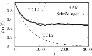
The approximation of HAM leads to the following expression for the population of the upper level:
| (55) |
where is defined by Eq. (50) and we have introduced a further relaxation rate:
| (56) |
On the other hand, the TCL master equation (53) gives:
| (57) |
Thus, the TCL master equation predicts an exponential relaxation of the populations to zero, while the solution obtained by means of HAM approaches the stationary population
| (58) |
To judge the quality of the various approximations we have performed numerical solutions of the full Schrödinger equation corresponding to the Hamiltonian defined by Eqs. (35) and (36). The initial state has been taken to be of the form , where the environmental state represents a superposition of the states of the lower band with independent Gaussian distributed random amplitudes of zero mean and equal variances. For certain parameter ranges we find an excellent agreement of the HAM prediction with the simulation results. An example is shown in Fig. 2. Note that for the parameters of this figure we have , such that the standard Markov condition (54) is very well satisfied.
We conclude that although the standard Markov condition (54) is fulfilled the Markovian master equation (53) does not yield a good approximation of the dynamics for intermediate and long times. In particular, its prediction for the stationary state is totally wrong. The important point to note is that, in order to judge the quality of the Markov approximation, an analysis of the contributions of higher orders is indispensable. We also note that the same problem occurs if one uses the Nakajima-Zwanzig master equation.
IV.2.3 The master equation of fourth order and failure of the Born-Markov approximation
To understand the failure of the Born-Markov approximation we investigate the fourth order of the TCL expansion. The contribution of fourth order to the TCL generator is given by Eq. (16). One finds that this contribution is determined by the two-point correlation function (49) and by the four-point correlation function:
| (59) |
The analysis shows that this function has two sharp peaks of width at , and at , , and may be approximated, under the conditions of the previous section, by the expression:
| (60) | |||||
The double-peak structure of the four-point correlation expressed by Eq. (60) has decisive consequences. With the help of the correlation functions given above the master equation of fourth order in the coupling is found to be:
| (61) | |||||
where
| (62) |
Equation (61) is a master equation with time-dependent relaxation rates and . The second-order contribution to the rate is given by , while the fourth order yields the contribution . Therefore, the fourth-order term of the TCL generator is small compared to the second-order term only if the times considered satisfy the additional condition
| (63) |
Thus we see that the occurrence of terms proportional to is responsible for strong deviations from the Markovian behavior. These terms are due to the double-peak structure of the four-point correlation function . We remark that this structure is markedly different to the usual situation of the coupling of an open system to a Bosonic field vacuum, for example. In this case has only a single peak and, hence, the above phenomenon of strong deviations from the Markovian dynamics for weak couplings does not occur.
The master equation (61) yields the coherences:
| (64) |
and the populations:
| (65) |
For we find the expansion:
which is seen to coincide with the corresponding short-time expansion of the HAM approximation given by Eq. (55). Thus we conclude that the TCL expansion based on the standard projection reproduces the short-time behavior predicted by HAM within the given orders. Correspondingly, the TCL approximation of fourth order clearly improves the approximation for short times, but leads to un-physical results for longer times and diverges in the limit , as is illustrated in Fig. 2. We note that a similar situation occurs for the spin star model studied in Ref. BURGARTH.
Summarizing, the fourth order clearly indicates that the TCL expansion does not converge uniformly in . It only provides a short-time expansion of the dynamics. As a result of the emergence of terms which are given by powers of , it is impossible to obtain valid predictions on the long-time dynamics if one truncates the TCL series at any finite order.
IV.3 TCL expansion using the correlated projection superoperator
In view of the above analysis the following question arises: Is it possible to construct a new projection superoperator whose corresponding TCL expansion yields the full prediction of HAM already in lowest order, and leads to a systematic expansion around HAM in higher orders? To answer this question we consider the following projection superoperator:
| (66) | |||||
This projection belongs to the class of superoperators introduced in Eq. (7). By this ansatz the total system’s state is approximated by a separable but non-factorizing state. The dynamical variables are the un-normalized density matrices and which are correlated with the projections onto the lower and the upper band, respectively. The reduced density matrix of the two-state system is found with the help of Eq. (9):
| (67) |
Assuming that the initial state is of the correlated form
| (68) |
we have and the inhomogeneous term of the TCL equation (10) vanishes.
IV.3.1 The second-order master equation
Using the new projection superoperator (66) we get the following second-order TCL equation:
| (69) | |||||
where the TCL generator takes the form:
| (70) | |||||
Combining Eqs. (69) and (70) and assuming again we find the equations of motion:
| (71) | |||||
| (72) |
This is a coupled system of first-order differential equations for the two density matrices and . The elements of these matrices are written as
| (73) |

The equations (71) and (72) can now be used to derive an equation of motion for the reduced density matrix, making use of Eq. (67). First, we get from Eq. (72):
| (74) | |||||
| (75) |
We assume again that initially only the lower band is populated:
| (76) |
It thus follows from Eq. (74) that
| (77) |
From Eq. (71) we find
| (78) |
From Eqs. (78) and (75) we see that the quantity is constant. With the help of the initial condition (76) we thus have
| (79) |
Substituting this into Eq. (78) we find:
| (80) |
Since because of Eq. (77), we finally arrive at the equation of motion for the populations:
| (81) |
In a similar manner one is led to the equation of motion for the coherences:
| (82) |
The dynamics of the reduced density matrix is thus determined by Eqs. (81) and (82). These are time-local first-order differential equations with constant coefficients. They are identical to the equations of motion obtained using HAM. In particular, the solution of Eq. (81) is given by the expression (55). Hence, we conclude that the lowest order of the TCL expansion with the projection superoperator introduced in Eq. (66) indeed reproduces the HAM prediction.


We observe that the dynamics of the populations is strongly non-Markovian because of the presence of the initial condition on the right-hand side of Eq. (81). This term expresses a pronounced memory effect, namely it implies that the dynamics of the populations never forgets its initial data. Note also that the dynamics of the reduced density matrix is not in Lindblad form and does even not represent a semigroup. It does, however, lead to a positive dynamical map, as can easily be verified.
In the transition from Eq. (70) to the Eqs. (71) and (72) we have assumed for simplicity that the times considered satisfy the condition . Without this condition the master equations (71) and (72) must be replaced by
| (83) | |||||
| (84) | |||||
These equations describe the full time dependence as it is predicted by the TCL expansion in second order. They lead to the following populations of the upper level:
| (85) |
where
| (86) |
and the function is given by Eq. (51).
In Figs. 3, 4, and 5 we compare the result given by Eq. (85) with the prediction of HAM and with numerical simulations of the Schrödinger equation. The figures clearly show that already the lowest order of the TCL expansion with the new projection superoperator gives a good approximation of the dynamics. It not only yields the correct stationary state, but also reasonable predictions on the relaxation times even for rather strong couplings, where deviations from the HAM result are large. Note that the rates of Fig. 3 differ from those of Fig. 5 by a factor of , and that the parameters of Fig. 5 correspond to the ratio .
IV.3.2 The master equation of fourth order
We have seen that the lowest order of the TCL expansion obtained with the help of the correlated projection superoperator is capable of reproducing the prediction of the HAM approximation, and even improves this approximation for larger couplings. The question is now: What happens in higher orders of the expansion? As our numerical simulations indicate, higher-order corrections should be small for all times. We show that, by contrast to the case of the standard projection, this is indeed the case.
The fourth-order contribution to the TCL generator is obtained by using the projection superoperator defined by Eq. (66) in the general expression (16). One finds:
Here, is again a function which is sharply peaked at and may be replaced by the delta function for times which are large compared to the inverse band width. The decisive point is the following. When carrying out the three-fold time integrations in the above expression, no terms emerge which grow like powers of . This is due to the fact that the integrands do not contain terms of the form . As a result, the contribution from remains small for all times , and the limit of the generator exists.
To illustrate this point let us model the function by
| (87) |
which approaches for infinite band width. The time-integrations may then easily be carried out to give:
Hence we see that becomes time-independent for and that the fourth order of the expansion leads to the equations of motion:
| (88) | |||||
| (89) | |||||
where we have introduced the rates:
| (90) | |||||
| (91) | |||||
| (92) | |||||
| (93) | |||||
| (94) |
This shows that the fourth order merely yields corrections of order to the equations of motion found in second order. Thus, as expected the TCL series obtained with the correlated projection superoperator indeed leads to a systematic perturbation expansion around the approximation suggested by HAM.
We finally mention that the equations of motion for the populations of the reduced system in fourth order take the form:
| (95) |
which is easily solved to yield:
| (96) |
The interesting point to note is that the stationary state is identical to the one found in second order. Thus, the stationary state is not affected by the fourth-order corrections. However, the rate of the relaxation into the stationary state is found to be
| (97) |
which is seen to be larger than the relaxation obtained in second order.
V Conclusions
In this paper we have analyzed non-Markovian quantum processes by means of the time-convolutionless projection operator technique and of the Hilbert space average method. It has been demonstrated that by use of a class of projection operators which project onto correlated system-environment states, an efficient non-perturbative treatment of certain non-Markovian processes is possible. The correlated projections have been shown to correspond to the idea of a best guess underlying the approximation of HAM.
The general mathematical formalism of the projection operator techniques does not tell us which projection superoperator should be used for a given system-environment model. The choice of an appropriate projection depends on the structure of the model under study and must be based on physical considerations. The aim is of course an efficient description, i. e., a description which can be expected to yield accurate results even in low orders of the coupling. Once a certain projection has been chosen, one can use the perturbation expansion in order to check explicitly whether or not higher orders remain small and, thus, whether or not enables a computationally efficient treatment of the reduced dynamics.
We emphasize that the projection operator techniques yield an expansion of the equations of motion for the relevant variables , and not an expansion of these variables itself. Different projection superoperators lead to different sets of relevant variables and, hence, to equations of motion with completely different structures. Consequently, the usage of different projections implies a complete re-organization of the perturbation expansion. This point has been demonstrated here by means of a specific system-environment model. As we have seen, the TCL technique which is based on the correlated projection superoperator yields accurate results for this model already in lowest order, while the standard TCL procedure fails in any finite order of the coupling.
Our results suggest applications to other models showing strong non-Markovian effects. For example, it is clear that the class of correlated projections introduced here may also be applied to a generalization of the model studied in Sec. IV which involves any number of well-separated environmental energy bands.
In Sec. II.1 we have formulated two general conditions for suitable superoperators . The first one [Eq. (3)] is simply the condition that the map be a projection operator. The second condition [Eq. (4)] requires that the projection of any state of the composite system contains the full information which is necessary to extract the reduced density matrix from the relevant variables. It is easy to construct classes of superoperators which satisfy these two conditions and are even more general than the class of correlated projections investigated here. As mentioned already the latter project the total state onto a separable, classically correlated system-environment state. This suggests exploiting the possibility of using superoperators which project onto nonseparable, entangled quantum states. In this way one might be able to investigate the dynamical significance of entanglement in non-Markovian quantum processes.
Acknowledgements.
We thank G. Mahler for fruitful discussions on this subject. Financial support for M. Michel and J. Gemmer by the Deutsche Forschungsgemeinschaft is gratefully acknowledged.References
- (1) H. P. Breuer and F. Petruccione, The Theory of Open Quantum Systems (Oxford University Press, Oxford, 2002).
- (2) D. F. Walls and G. J. Milburn, Quantum Optics (Springer-Verlag, Berlin, 1994).
- (3) U. Weiss, Quantum Dissipative Systems (World Scientific, Singapore, 1999).
- (4) P. Pechukas and U. Weiss (guest editors), Quantum Dynamics of Open Systems, Chemical Physics, Special Issue, Vol. 268, Nos. 1-3 (2001).
- (5) M. A. Nielsen and I. L. Chuang, Quantum Computation and Quantum Information (Cambridge University Press, Cambridge, 2000).
- (6) D. D. Awschalom, D. Loss, and N. Samarth (eds.), Semiconductor Spintronics and Quantum Computation, Series on Nanoscience and Technology (Springer-Verlag, Berlin, 2002).
- (7) V. B. Braginsky and F. Ya. Khalili, Quantum Measurement (Cambridge University Press, Cambridge, 1992).
- (8) D. Giulini, E. Joos, C. Kiefer, J. Kupsch, I.-O.Stamatescu, and H. D. Zeh, Decoherence and the Appearance of a Classical World in Quantum Theory, second edition (Springer-Verlag, Berlin, 2003).
- (9) J. Gemmer, M. Michel, and G. Mahler, Quantum Thermodynamics, Lecture Notes in Physics Vol. 657 (Springer-Verlag, Berlin, 2004).
- (10) J. Gemmer, A. Otte, and G. Mahler, Phys. Rev. Lett. 86, 1927 (2001).
- (11) V. Gorini, A. Kossakowski, and E. C. G. Sudarshan, J. Math. Phys. 17, 821 (1976).
- (12) V. Gorini, A. Frigerio, M. Verri, A. Kossakowski, and E. C. G. Sudarshan, Rep. Math. Phys. 13, 149 (1978).
- (13) H. Spohn, Rev. Mod. Phys. 53, 569 (1980).
- (14) G. Lindblad, Commun. Math. Phys. 48, 119 (1976).
- (15) S. Nakajima, Progr. Theor. Phys. 20, 948 (1958).
- (16) R. Zwanzig, J. Chem. Phys. 33, 1338 (1960).
- (17) H. Grabert, Projection Operator Techniques in Nonequilibrium Statistical Mechanics, Springer Tracts in Modern Physics Vol. 95 (Springer-Verlag, Berlin, 1982).
- (18) R. Kubo, M. Toda, and N. Hashitsume, Statistical Physics II. Nonequilibrium Statistical Mechanics, (Springer-Verlag, Berlin, 1991).
- (19) F. Shibata, Y. Takahashi, and N. Hashitsume, J. Stat. Phys. 17, 171 (1977).
- (20) S. Chaturvedi and F. Shibata, Z. Phys. B 35, 297 (1979).
- (21) F. Shibata and T. Arimitsu, J. Phys. Soc. Jap. 49, 891 (1980).
- (22) C. Uchiyama and F. Shibata, Phys. Rev. E 60, 2636 (1999).
- (23) A. Royer, Phys. Lett. A 315, 335 (2003).
- (24) T.-M. Chang and J. L. Skinner, Physica A 193, 483 (1993).
- (25) L. D. Blanga and M. A. Despósito, Physica A 227, 248 (1996).
- (26) H. P. Breuer, B. Kappler, and F. Petruccione, Ann. Phys. (N.Y.) 291, 36 (2001).
- (27) H. P. Breuer, D. Faller, B. Kappler, and F. Petruccione, Europhys. Lett. 54, 14 (2001).
- (28) H. P. Breuer, B. Kappler, and F. Petruccione, Phys. Rev. A 59, 1633 (1999).
- (29) A. Shabani and D. A. Lidar, Phys. Rev. A 71, 020101(R) (2005).
- (30) R. Kubo, J. Math. Phys. 4, 174 (1963).
- (31) A. Royer, Phys. Rev. A 6, 1741 (1972).
- (32) N. G. van Kampen, Physica 74, 215 (1974).
- (33) N. G. van Kampen, Physica 74, 239 (1974).
- (34) M. Esposito and P. Gaspard, Phys. Rev. E 68, 066112 (2003).
- (35) B. M. Garraway, Phys. Rev. A 55, 2290 (1997).
- (36) B. M. Garraway, Phys. Rev. A 55, 4636 (1997).
- (37) A. Imamoglu, Phys. Rev. A 50, 3650 (1994).
- (38) H. P. Breuer, Phys. Rev. A 70, 012106 (2004).
- (39) A. A. Budini, e-print eprint quant-ph/0510085.
- (40) J. Gemmer and M. Michel, Europhys. Lett. 73, 1 (2006).
- (41) J. Gemmer and M. Michel, Physica E 29, 136 (2005).
- (42) G. Alber, T. Beth, M. Horodecki, P. Horodecki, R. Horodecki, M. Rötteler, H. Weinfurter, R. Werner, and A. Zeilinger, Quantum Information (Springer-Verlag, Berlin, 2001).
- (43) R. F. Werner, Phys. Rev. A 40, 4277 (1989).
- (44) J. Gemmer and G. Mahler, Euro. Phys. J. B 31, 249 (2003).
- (45) H. P. Breuer, D. Burgarth, and F. Petruccione, Phys. Rev. B 70, 045323 (2004).