Quantum Walk with a time-dependent coin
Abstract
We introduce quantum walks with a time-dependent coin, and show how they include, as a particular case, the generalized quantum walk recently studied by Wojcik et al. [Phys. Rev. Lett. 93, 180601(2004)] which exhibits interesting dynamical localization and quasiperiodic dynamics. Our proposal allows for a much easier implementation of this particular rich dynamics than the original one. Moreover, it allows for an additional control on the walk, which can be used to compensate for phases appearing due to external interactions. To illustrate its feasibility, we discuss an example using an optical cavity. We also derive an approximated solution in the continuous limit (long–wavelength approximation) which provides physical insight about the process.
1 Introduction
Quantum walks (QWs) [1, 2] constitute a promising ingredient in the research of quantum algorithms [3] but have also an intrinsic interest, reinforced through their connection with quantum cellular automata [2] and with phenomena such as Anderson localization or quantum chaos [4, 5, 6].
Both in the discrete or continuous version, QWs provide a mean to explore all possible paths on a lattice in a parallel way, which is natural for quantum evolution, together with constructive quantum interference along the paths. Thus they can allow the development of probabilistic algorithms in a more efficient way than their classical counterparts [7]. It is therefore crucial to fully explore the possibilities offered by QWs, especially in connection with their physical implementation.
Modified QWs can give rise to new physical phenomena, along with more efficient algorithmic applications. Different variations of the standard discrete time QW have been proposed, including QWs with two entangled particles [8] or entangled coins [9], multi–states QWs [10, 11], as well as QWs with alternation of different quantum coins in a certain sequence [12]. More interesting to us are the generalized QWs that modify the time evolution by the acquisition of position–dependent phases by the walker at every step [4, 5, 6]. Those generalizations show phenomena that differ from the typical linear spreading of the wave function in the standard QW, such as quantum resonances and dynamic localization.
Within this spirit, we explore a modification on the standard coined QW, which consists on the introduction of a time-dependent coin. As we discuss, this modification introduces new possibilities on the walk which are worth investigating. Here we concentrate on a particular time dependent coin that leads to QW equations nearly identical to those corresponding to the generalized QW introduced by Wojcik et al. [5] (see also [4, 6]). Our approach presents the advantage that the corresponding modifications are made on the coin alone, which is a simple one-qubit system, in contrast to the original proposal, which requires operations to be performed on a large system (the Hilbert space of the walking particle). Moreover, using a time-dependent coin can be used as a control mechanism to compensate for a phase arising from some external influence. We illustrate this idea with an example.
This paper is organized as follows. In Section 2 we introduce the basic idea of a time-dependent coined QW and relate it to previous works. In Section 3, we first review the main aspects of the generalized QW introduced by Wojcik et al. [5], and then show how an extra transformation (with respect to the standard coined QW) on the walking particle, can be encoded into a time-dependent coin, and show the equivalence between the obtained generalized QW and that of [5]. We also discuss the utility of a time-dependent coin as a control mechanism. In Section 4, we show how this generalized QW could be implemented in an optical cavity. Then, in Section 5, we derive an approximated continuous limit, a long wave–length approximation to this time-dependent QW, which is appropriate for describing dynamic localization. Finally, in Section 6 we summarize our main results.
2 Time-dependent coined walks
The standard QW corresponds to the evolution on a one-dimensional lattice of a quantum system (the walker) coupled to a bidimensional system (the coin), under repeated application of a pair of discrete operators. Let be the Hilbert space of the walker, with a basis of ; and let be the Hilbert space of the coin, with basis . The state of the total system belongs to the space and, at a given time, can be expressed as
| (1) |
The evolution of the system is governed by two operators: (i) an arbitrary unitary transformation acting on , which can be any unitary 2x2 matrix and is usually chosen as
| (2) |
(with the balanced Hadamard coin is recovered); and (ii) the conditional displacement operator acting on
| (3) | |||||
| (4) |
Altogether, they produce the evolution from instant to given by
| (5) |
In this paper, we introduce the idea of a modified QW, where the coin changes during the evolution, i.e. . In this case, the evolution from instant to is defined by
| (6) |
A particular case of this would be the proposal in [12], in which two fixed standard coins were alternated in a given sequence, leading to a sub-ballistic wave-function spreading for some particular choices of the coin series. In order to be more specific, we study the effect of a time-dependent coin of the special form
| (7) |
Notice that (7) can be obtained as the sequence of two operations, i.e.,
| (8) |
with
| (9) |
and given by (2).
Again, is quite a general function. In this article we shall restrict ourselves to a particular case that, as commented above, leads to a generalized QW which is nearly identical to that analyzed in Ref. [5]. Other possibilities will be considered in a future work.
3 Using time-dependent coins to implement dynamic localization and quasiperiodic dynamics
Recently, Wojcik et al. [5] (see also [4, 6]) showed that a generalization of the QW (GQW in the following) in which a position-dependent phase was acquired by the walker with each evolution step, produces quasiperiodic dynamics and localization effects. There is a physical reason for introducing : the walker is a physical system that evolves in time, and this evolution can introduce such phases, via e.g. external interactions.
Here we show that such generalization can in fact be recast as a QW with a time-dependent coin. We concentrate here on the GQW of [5], which is equivalent to that of [4], but our approach can easily be shown to cover also Romanelli’s et al. proposal [6]. In fact, the only difference in the dynamical equations, with respect to [4, 5], is that the position dependent phase in [6] goes like .
3.1 GQW
Let us briefly present the GQW introduced in [5]. We first define the discrete position operator such that
| (10) |
and, related to this one, the phase operator
| (11) |
where is a constant. Following [5], the evolution of the system is governed by
| (12) |
The state of the system at a given time can be expressed as
| (13) |
from which it is easy to obtain
| (14) | |||||
| (15) |
From the solution of these equations one can evaluate the probability of finding the walker at the lattice point at iteration by using
| (16) |
We now briefly summarize the main features of the solutions of Eqs. (14,15). Wojcik et al. [5] found that for rational values of dynamical localization, shown by a ’quasiperiodic’ behavior of the standard deviation of the probability distribution, is observed during a transient regime, but for long enough times a ballistic diffusion occurs. For irrational values of , on the contrary, the diffusion becomes suppressed, and the walk shows dynamic localization around the starting point for arbitrarily long . Let us consider the case of a rational in more detail.
First we notice that the probability distribution is invariant under the change
| (17) |
Then, if we focus on rational values of , we can restrict the study to
| (18) |
where is an irreducible fraction. Moreover, the study can be limited to even values of , since given a case with odd , there is a value with even denominator leading to the same probability distribution, as a consequence of symmetry (17).

Keeping this in mind, a numerical analysis of Eqs. (14,15) shows that, given an even , the solution of the GQW shows a quasiperiod during the above-mentioned transient regime. The duration of this transient, i.e., the number of quasiperiods that it exhibits, turns out to be larger the larger is . In other words, the probability that the walker returns to the initial position after one quasiperiod, () with , increases with , as we show in Fig. 1. This figure clearly shows that the loss of localization takes place more slowly for larger values of .
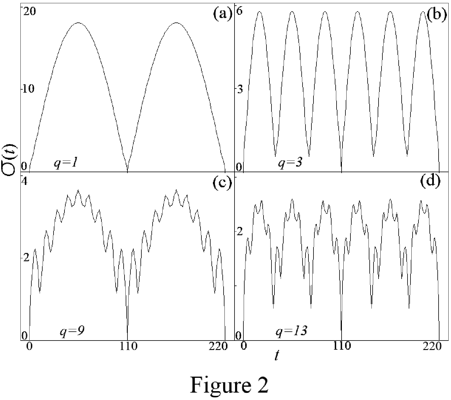
Apart from this oscillation of quasiperiod , the standard deviation of the probability distribution shows a faster secondary oscillation that depends on . In fact, one finds secondary oscillations within each period of the main oscillation. These secondary oscillations are more pronounced the smaller is and the larger is . This is clearly appreciated in Fig. 2, where we show the evolution of for and four different values of . Notice how the GQW returns (only approximately, remind this is a transient behavior) to the initial condition, , when , oscillating times between and .
3.2 An alternative approach
Here we present our alternative approach. Let us define
| (19) |
It is straightforward to show that the following relationship holds
| (20) |
Repeated use of the above expression, together with the evolution Eq. (12), leads to a modified form of the evolution equation, which can be expressed as
| (21) |
where verifies
| (22) | |||||
| (23) |
and is a time-dependent coin operator, defined as
| (24) |
i.e., , c.f. Eq. (7), with . By this simple procedure we have demonstrated that the generalization of the QW introduced in Ref. [5] can be obtained by introducing a suitable time dependent coin. Although the probability amplitudes are not identical to those of the GQW due to the phase factors appearing in Eq. (21), the probability distributions are the same obtained either with or with , and both descriptions are thus equivalent from this point of view.
The equivalence nevertheless breaks down for the QW on the circle, as the phase added in [5] depends on the position, so that a difference may arise in the circle when passing from position to position .
Now we write down explicitly the equations of evolution for our alternative approach. By performing a decomposition analogous to Eq. (13), the equations of evolution become
| (25) | |||||
| (26) |
which are equivalent to Eqs.(14,15), as Eq. (21) provides the connection between both descriptions, which reads
| (27) |
We now transform the coupled equations (25) and (26) into space-time recursive equations for and , where both components are decoupled. We start from
| (28) | |||||
| (29) |
and making use of
| (30) |
we obtain, after some algebra
| (31) |
or, equivalently,
| (32) | |||||
| (33) |
Finally, the probability of finding the walker at the lattice point at iteration is given by
| (34) |
Since and , there is no difference between the probability distribution for the QW on a line calculated with Eqs. (25, 26) or with Eqs. (14, 15), as already commented.
3.3 The time-dependent coin as a control mechanism
In this subsection we discuss how a time-dependent coin can be used to gain control over a possible phase arising during the walk, as a consequence of additional interactions [4]. We illustrate this idea with an example which shows that, at least in some cases, the position-depending phase acquired between two steps in the walk could be canceled by an appropriate action on the coin.
Let us assume that the walker is subjected to the effect of the GQW defined by Eq. (12). We have shown in the previous subsection that this kind of QW is equivalent (modulo a final phase) to one with a time-dependent coin. Intuitively, if one wants to compensate for the phases acquired during the GQW, one should replace the coin operator by a time-dependent operator defined by . In this way, the evolution is governed by
Using the properties given in section 3.2, one obtains:
| (35) |
Showing that the combined action of the phase operator and the time-dependent coin defined above, is equivalent (up to a phase give by the action of ) to the standard quantum walk introduced in section 2. In other words, Eq. (35) can be written, when decomposed in the basis, as
where . The coefficients then correspond to Eq. (35), whereas stand for the standard QW. In this way, the complex dynamics arising from the GQW translates into a trivial phase.
4 Implementing the generalized quantum walk
Along recent years there have been many proposals for the experimental implementation of QWs. These cover both systems whose dynamics can be described only within the framework of quantum mechanics [13, 14, 15, 16, 17, 18, 19] as well as setups whose description does not require quantum mechanics [20, 21, 22, 23, 24]. In fact, the QW on the line was nearly implemented in an optical cavity [25], as it was highlighted in [21] and fully discussed in [22]. Although an experimental realization of the QW using only classical means has been communicated recently [26], it is a fact that there has been little experimental research about this process.
Here we comment on how the GQW we are studying could be implemented in an optical cavity. We follow our approach to the GQW as it is more easily implementable than the original proposal by Wojcik et al. [5]. This is due to the fact that with our approach it is only needed to modify the unitary transformation acting on the qubit, which is a 2–dimensional system, while the original proposal [5] implies acting on all the points of the lattice.
In [21, 22], it was shown that the QW on the line can be implemented by the frequency of a quasi–monochromatic field, e.g. an optical pulse of appropriate duration, inside an optical cavity. As stated, in this classical implementation the role of the walker is played by the field frequency, and the role of the coin can be played, e.g., by the field polarization. The simplest scheme is that represented in Fig. 3 [21], without EOMbis (see below for the role of this element): The electrooptic modulator (EOM) implements the displacement operator, Eqs. (3, 4), by increasing (decreasing) the frequency of the horizontal (vertical) polarization component of the field. As for the unitary transformation, , it is performed by a half–wave plate (HWP) with suitably oriented fast axis [27]. Thus in a cavity round-trip a step of the QW is performed. The optical cavity allows the repetition of the process through feedback. The number of steps of the QW that can be implemented depends on factors such as the technical limitations of the EOM and on the losses of the cavity (this last factor could be compensated by introducing gain in the cavity, as in [25]). We address the interested reader to [22] for more details. Let us remark that this simple scheme is very close to what was actually performed in the experiment of Bouwmeester et al. [25] (see [22] for a full discussion).

We can take this scheme as a basis for the implementation of the generalized QW. In order to perform the GQW, one needs to implement the time dependent unitary transformation , Eq. (24). This can be done by adding one optical element between EOM and HWP to implement , Eq. (19). This is the role played by EOMbis in Fig. 3. Consider first a single step of the GQW, i.e., that corresponding to iteration . For this one must implement , which can be done in a straightforward way: The implementation simply consists in the addition (subtraction) of to the phase of the horizontal (vertical) polarization component of the field. This can be easily carried out, e.g., by introducing a second EOM, EOMbis in Fig. 3, to which a suitable (constant) voltage is applied. Now, in order to implement , this added (subtracted) phase must be increased at each cavity round-trip, what is done by applying a staircase voltage to EOMbis (represented in Fig. 3): The voltage must remain constant while the light pulse is traversing EOMbis, in order to modify the phase and not the field frequency, and then be rapidly increased for the phase increment takes the value in the subsequent round-trip. We think that this simple scheme, which can be implemented with current technology (it consists in adding a single element to the device already used in [25]), could allow the experimental investigation of the GQW.
5 A long–wavelength approximation to the generalized quantum walk
Up to now we have shown how the GQW can be alternatively produced by means of a time dependent coin, how it could be experimentally implemented, and also how the time dependent coin can be used in the presence of phases in the walker displacement for controlling or tuning the GQW. Now we will try to get some insight into the physics of the GQW, by deriving a continuous version through a long–wavelength approximation. In this way we derive a wave equation that constitutes a continuous propagation analog of the GQW. The analogy helps to visualize the kind of physical process that produces the GQW.
We introduce here a long wave approximation by following the same lines as in [21, 28]. Our starting point is the recurrence equation
| (36) |
where stands for both and . In this way, Eq. (36) corresponds to Eqs. (32) and (33) after the factors on the left hand side have been neglected 11 1 This approximation is perfectly justified. Perhaps it is more clearly seen if instead of the unitary transformation (24), one uses In this case, the exponential factors we are neglecting do not appear on the left-hand side, as in Eqs. (32, 33), but on the right–hand side of these equations in the form which can be approximated by for large enough .. In [21, 28] it was shown that it is necessary to introduce two discrete fields in order to preserve the symmetry of the QW. Thus we define the new fields through
| (37) |
By inserting this definition into Eq. (36), one immediately obtains
| (38) |
which is convenient to rewrite in the form
| (39) | |||||
Denoting by and the continuous space and time variables, and by and the spacing between lattice points and time between iterations, we can define the adimensional continuous variables and and think of Eq. (39) as the discretization of the following partial differential equation
| (40) | |||||
which constitutes a continuous limit of the GQW.
Taking into account Eq. (37), and the fact that the discrete fields describe both and , the continuous versions of these fields, which we denote by and , are calculated through
| (41) | |||||
| (42) |
with and the solutions of Eq. (40) for and , respectively (see the Appendix).
The long-wavelength approximation consists in retaining the lowest order in Eq. (40). Importantly, we further neglect the third temporal derivative. We address the reader to the Appendix for full details. After all of this, we are left with
| (43) |
where the new fields defined by
| (44) |
have been introduced. This equation can be solved analytically, and the explicit solution is derived in the Appendix.
We notice that Eq. (43) has time–periodic coefficients and, consequently, as we have retained only the first derivative with respect to time, their solutions are time–periodic. We can then expect that the solutions of Eq. (43) describe approximately the periodic solutions of the GQW, which appear when is an irrational multiple of , but not the quasiperiodic solutions ( a rational multiple of ) except in the cases with very long quasiperiod. Obviously, this partial description of the solutions is the price to be paid after neglecting the third time derivative in Eq. (40).
Before discussing the physical meaning of Eq. (43), let us first compare the exact solution of the time-dependent coined QW, Eqs. (32,33), with the approximated continuous solution we have just derived. In order to do that, we have chosen a value for the phase ( ) for which the quasiperiod is very large ( in this case). We have taken symmetrical initial conditions too (i.e. and ). For the continuous version, we will take to be a superposition of gaussians with a width (see the Appendix for details).

Fig. 4 shows both the exact probability distribution , Fig. 4(a), and the approximated continuous solution, Fig. 4(b), for time running from to , at intervals of time units. For the exact probability distribution only even points of the lattice, for which the probability is non zero, are shown and joined for an easier visualization. We have chosen to evaluate . One sees how similar these distributions are, except for close to , where the continuous distribution is wider. Then, the approximated continuous solution can be considered as a good approximation for cases with periodic behavior or with quasiperiodic behavior with very long transients.
Fig. 4 is complemented with Fig. 5, where we show: the exact (with even points joined again) on the top row; the approximated on the bottom row; and finally, in the middle row, the same as in the bottom row (i.e., the long–wavelength approximation) but evaluated only at discrete position values for a better comparison of the previous two results. We do this for three different time values (, , ). Again, as in Fig. 4, one sees how and are very similar, except near the semiperiod.

Finally, we compare the evolution of the quadratic deviation in position using both the exact distribution and the continuous distribution in Fig. 6. We continue in the dynamic localization case with , and compare the exact case (a) with five continuous limit cases (b) corresponding to , , , and . Notice that the behaviors of both the exact case and the continuous limit are similar, except for the fact that with the continuous limit one obtains an “excess of quadratic deviation”, specially within the proximity of the semiperiod, because of the already mentioned problem with the width.

The above results show that the continuous long–wavelength approximation, Eq. (43), is a good qualitative approximation, even a reasonably good quantitative approximation, to the GQW in the dynamical localization regime. We have already commented that the failure in describing the diffusive dynamics occurring in the GQW for rational values of is due to the neglect of the third order time derivative in deriving Eq. (43), an approximation made in order to obtain analytical expressions.
Eq. (43) is a linear wave equation describing the propagation of waves in a medium with special dispersion properties: The dispersion coefficients (those multiplying the higher order spatial derivatives) are time periodic, as well as the wave group velocity (the coefficient multiplying the first order spatial derivative). Thus, the essential for dynamical localization correspond to the vanishing of the time-averaged group velocity, while its periodic time dependence is the responsible for the ”bouncing” of the probability distribution, see Fig. 4. As for the rest of spatial derivatives, they introduce a distortion on the probability distribution (due to dispersion) that turns out to be reversible again because of the time periodicity of the coefficients. Certainly, a group velocity that changes its sign periodically is not a common situation for waves, but the analogy that Eq. (43) establishes provides an alternative physical picture that, as we have seen, helps to understand dynamical localization in the GQW and could help for the search of propagation phenomena in which this phenomenon could manifest. In this sense, it is interesting to notice the similarity between this equation and that describing beam propagation in waveguides with a bent axis [30], an optical process in which Bloch oscillations and dynamical localization have been recently experimentally observed [31] (we note that in [5] the connection between the GQW and Bloch oscillations was put forward).
6 Conclusions
In this article we have introduced QWs with time dependent coins. We have considered a particularly simple case that turns out to be equivalent to the generalized QW (GQW) introduced by Wojcik et al. [5]. This GQW exhibits very striking dynamical properties, particularly dynamical localization. We have shown how our alternative proposal can be used as a control mechanism. In addition, this time-dependent QW is particularly interesting from the implementation point of view, as only simple actions on the coin–qubit are required for that.
We have also obtained a long–wavelength continuous approximation of the GQW equations that have allowed us the derivation of an approximated explicit continuous solution that works quite well during the dynamic localization regime. The continuous equation from which this solution was derived is a linear partial differential equation describing pulse propagation in a dispersive medium with periodical time dependence in the dispersion coefficients. This continuous limit has lead us to interpret the main feature of GQW, the dynamic localization, as a propagating solution in the dispersive medium with null mean value of its group velocity.
Acknowledgments
This work has been financially supported by Spanish Ministerio de Educación y Ciencia and European Union FEDER through project FIS2005-07931-C03-01, and by Grants FPA2002-00612, AYA2004-08067-C03, FPA2005-00711 and GV05/264.
7 Appendix
Now we perform the long-wavelength approximation that consists in retaining terms up to in Eq. (40), i.e.
| (45) | |||||
The third-order derivative on the left–hand side makes it hard to obtain an analytical solution. In the case of the standard QW, the third time derivative was approximated by making use of the lowest order expansion ( in Eq.(40)) [21], but in our case the time–dependent coefficient of the remaining linear term renders this approach useless. We then make a further approximation and neglect the third order derivative in time. By making the change
| (46) |
one obtains
| (47) |
which we pass to solve here.
In order to solve the integral (48), one must fix , i.e., . Following [21], we assume that
| (51) |
and then, by using Eq. (37),
| (52) |
Notice that is evaluated from Eqs. (25, 26) once the initial condition has been fixed.
Here we consider, as usual, that the walker is initially located at the origin of the lattice, i.e., except for . Then in the continuous limit we take
| (53) |
where
| (54) |
with a normalization constant that will be omitted in the following. As in [21] we are assuming that Eq. (40) is correct only for the long–wavelength components by taking an initial condition that “smears out” the lower–wavelength components.
References
- [1] Y. Aharonov, L. Davidovich, and N. Zagury, Phys. Rev. A 48 1687 (1993).
- [2] D. Meyer, J. Stat. Phys. 85, 551 (1996).
- [3] For reviews, see J. Kempe, Contemp. Phys. 44, 307 (2003); A. Ambainis, Int. J. Quantum Inform. 1, 507 (2003).
- [4] O. Buerschaper and K. Burnett, quant-ph/0406039.
- [5] A. Wojcik, T. Lukzak, P. Kurzynski, A. Grudka, and M. Bednarska, Phys. Rev. Lett. 93, 180601 (2004).
- [6] A. Romanelli, A. Auyuanet, R. Siri, G. Abal and R. Donangelo, Physica A 352, 409 (2005).
- [7] E. Farhi and S. Gutman, Phys. Rev. A 58, 915 (1998).
- [8] Y. Omar, N. Paunkovic, L. Sheridan, and S. Bose, quant-ph/0411065.
- [9] S.E. Venegas–Andraca, J.K. Ball, K. Burnett, and S. Bose, New J. Phys. 7, 221 (2005).
- [10] N. Inui and N. Konno, Physica A 353, 133 (2005).
- [11] N. Inui, N. Konno, and E. Segawa, Phys. Rev. E 72, 056112 (2005).
- [12] P. Ribeiro, P. Milman, and R. Mosseri, Phys. Rev. Lett. 93 190503 (2004).
- [13] B.C. Travaglione and G.J. Milburn, Phys. Rev. A 65, 032310 (2002).
- [14] W. Dür, R. Raussendorf, V.M. Kendon, and H.-J. Briegel, Phys. Rev. A 66, 052319 (2002).
- [15] B.C. Sanders, S.D. Bartlett, B. Tregenna, and P.L. Knight, Phys. Rev. A 67, 042305 (2003).
- [16] Z. Zhao, J. Du, H. Li, T. Yang, Z.-B Chen, and J.-W. Pan, e-print quant-ph/0212149.
- [17] T. Di, M. Hillery, and M.S. Zubairy, Phys. Rev. A 70, 032304 (2004).
- [18] K. Eckert, J. Mompart, G. Birkl, and M. Lewenstein, Phys. Rev. A 72, 012327 (2005).
- [19] G.S. Agarwal and P.K. Pathak, Phys. Rev. A 72, 033815 (2005).
- [20] M. Hillery, J. Bergou, and E. Feldman, Phys. Rev. A 68, 032314 (2003).
- [21] P.L. Knight, E. Roldán, and J.E. Sipe, Phys. Rev. A 68, 020301(R) (2003).
- [22] P.L. Knight, E. Roldán, and J.E. Sipe, Opt. Commun. 227, 147 (2003); erratum 232 (2004) 443.
- [23] H. Jeong, M. Paternostro, and M. S. Kim, Phys. Rev. A 69, 012310 (2004).
- [24] E. Roldán and J.C. Soriano, J. Mod. Opt. 52, 2649 (2005).
- [25] D. Bouwmeester, I. Marzoli, G.P. Karman, W. Schleich, and J.P. Woerdman, Phys. Rev. A 61, 013410 (2000).
- [26] B. Do, M.L. Stohler, S. Balasubramanian, D.S. Elliot, Ch. Eash, E. Fischbach, M.A. Fischbach, A. Mills, and B. Zwickl, J. Opt. Soc. Am. 22, 499 (2005).
- [27] R.J.C. Spreeuw, Phys. Rev. A 63, 062302 (2001).
- [28] P.L. Knight, E. Roldán, and J.E. Sipe, J. Mod. Opt. 51, 1761 (2004).
- [29] M. Miyagi and S. Nishida, Appl. Opt. 18, 678 (1979).
- [30] S. Longhi, D. Janner, M. Marano, and P. Laporta, Phys. Rev. E 67, 036601 (2003).
- [31] S. Longhi, M. Marangoni, R. Ramponi, P. Laporta, E. Cianci, and V. Foglietti, quant-ph/0511132.