Cloning of observables

Information may be effectively manipulated and transmitted by encoding symbols into quantum states. However, besides several advantages, the quantum nature of the transmitted signals entails some drawback, the most relevant owing to the so-called no-cloning theorem: Quantum information encoded in a set of nonorthogonal states cannot be copied [1, 2, 3]. In order to overcome this limitation an orthogonal coding may be devised, which however requires the additional control of the quantum channel since, in general, propagation degrades orthogonality of any set of input quantum signals.

A different scenario arises by addressing transmission of information encoded in the statistics of a set of observables, independently on the quantum state at the input. In a network of this sort there is no need of a precise control of the coding stage whereas, on the other hand, each gate should be transparent, i.e. should preserve the statistics of the transmitted observables. In this paper, we address the problem of copying information that has been encoded in the statistics of a set of observables. For this purpose we introduce the concept of cloning machine for classes of observables and analyze in details the constraint imposed by quantum mechanics to this kind of devices. Two forms of a no-cloning theorem for observables will be derived, and the connections with cloning of states and joint measurements will be discussed.

In the following we assume that information is encoded in the statistics of a set of qubit observables. A cloning machine for the given set is a device in which a signal qubit carrying the information interacts with a probe qubit via a given unitary with the aim of reproducing the statistics of each observable on both the qubits at the output. The chance of achieving this task, besides the choice of a suitable interaction, depends on the class of observables under investigation. In this paper we provide a full classification of cloning machines, based on the number of parameters needed to specify the class.

The paper is structured as follows: In Section 2 we introduce the concept of cloning machine for a class of observables and illustrate some basic properties. Then, the possibility of realizing a cloning machines for a given class is analyzed, depending on the number of parameters individuating the class. The results are summarized in two forms of a no-cloning theorem for observables. In Section 3 we analyze the connections between cloning of observables and joint measurements of noncommuting observables. Section 4 closes the paper with some concluding remarks.

We consider a device in which a signal qubit (say, qubit ”1”) is prepared in the (unknown) state $\varrho$ and then interacts, via a given unitary $U$, with a probe qubit (”2”) prepared in the known state ${\varrho_{p}}$. For a given class of qubit observables $\mathbf{X}\equiv\left\{{\rm X}(j)\right\}_{j\in{\cal J}}$ where ${\cal J}$ is a subset of the real axis and ${\rm X}(j)\in{\cal L}[{\mathbb{C}}^{2}]$, we introduce the concept of cloning as follows. A cloning machine for the class of observables $\mathbf{X}$ is a triple $(U,{\varrho_{p}},\mathbf{X})$ such that

where $\overline{\rm X}\equiv\hbox{Tr}_{1}\left[\varrho\>{\rm X}\right]$ is the mean value of the observable $X$ at the input and

are the mean values of the same observable on the two output qubits (see Fig. 1). The density matrix $R=U\>\varrho\otimes{\varrho_{p}}\>U^{\dagger}$ describes the (generally entangled) state of the two qubits after the interaction, whereas $I$ denotes the identity operator.

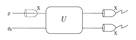
The above definition identifies the cloning of an observable with the cloning of its mean value. This is justified by the fact that for any single-qubit observable ${\rm X}$ the cloning of the mean value is equivalent to the cloning of the whole statistics. In fact, any ${\rm X}\in{\cal L}[{\mathbb{C}}^{2}]$ has at most two distinct eigenvalues $\{\lambda_{0},\lambda_{1}\}$, occurring with probability ${p_{0},p_{1}}$. For a degenerate eigenvalue the statement is trivial. For two distinct eigenvalues we have $\overline{\rm X}=\lambda_{1}p_{1}+\lambda_{0}p_{0}$ which, together with the normalization condition $1=p_{0}+p_{1}$, proves the statement. In other words, we say that the class of observables $\mathbf{X}$ has been cloned if a measurement of any ${\rm X}\in\mathbf{X}$ on either the two qubits at the output gives the same statistics as it was measured on the input signal qubit, independently on the initial qubit preparation.

A remark about this choice is in order. In fact, in view of the duality among states and operators on an Hilbert space, one may argue that a proper figure of merit to assess a cloning machine for observables would be a fidelity–like one. This is certainly true for the $d$-dimensional case, $d>2$, while for qubit systems a proper assessment can be also made in term of mean–value duplication, which subsumes all the information carried by the signal.

Our goal is now to classify cloning machines according to the number of parameters needed to fully specify the class of observables under investigation. Before beginning our analysis let us illustrate a basic property of cloning machines, which follows from the definition, and which will be extensively used throughout the paper.

Given a cloning machine $\left(U,{\varrho_{p}},\mathbf{X}\right)$, then $\left(V,{\varrho_{p}},{\mathbf{Y}}\right)$ is a cloning machine too, where $V=(W^{\dagger}\otimes W^{\dagger})\>U\>(W\otimes I)$ and the class ${\mathbf{Y}}=W^{\dagger}\mathbf{X}W$ is formed by the observables $Y(j)=W^{\dagger}X(j)\,W$, $j\in{\cal J}$. The transformation $W$ may be a generic unitary. We will refer to this property to as unitary covariance of cloning machine. The proof proceeds as follows. By definition $\overline{\rm Y}(j)={\rm Tr}_{1}[\varrho\>W^{\dagger}X(j)W]={\rm Tr}_{1}[W\,\varrho\,W^{\dagger}\,{\rm X}(j)]$. Then, since $\left(U,{\varrho_{p}},\mathbf{X}\right)$ is a cloning machine, we have

The same argument holds for $\overline{\rm Y}_{2}(j)$.

Another result which will be used in the following is the parameterization of a two-qubit transformation, which corresponds to a ${\rm SU}(4)$ matrix, obtained by separating its local and entangling parts. A generic two-qubit gate ${\rm SU}(4)$ matrix may be factorized as follows [4]:

where $\theta_{j}\in\mathbb{R}$ and the $\sigma_{j}$’s are the Pauli’s matrices. The local transformations $L_{1}$ and $L_{2}$ belongs to the ${\rm SU}(2)\otimes{\rm SU}(2)$ group, whereas $U_{\rm E}$ accounts for the entangling part of the transformation $U$. In our context, decomposition (3), together with unitary covariance of cloning machines, allows to ignore the local transformations $L_{1}$, which corresponds to a different state preparation of signal and probe qubits at the input. On the other hand, as we will see in the following, the degree of freedom offered by the local transformations $L_{2}$ will be exploited to design suitable cloning machines for noncommuting observables.

As we already pointed out in the previous sections there are no cloning machines for a two–parameter class of noncommuting observables (Theorem 2). Therefore, a question arises on whether, analogously to state–cloning, we may introduce the concept of approximate cloning machines, i.e. cloning of observables involving added noise. Indeed this can be done and optimal approximate cloning machines corresponding to minimum added noise may be found as well.

An approximate cloning machine for the class of observables $\mathbf{X}$ is defined as the triple $(U,{\varrho_{p}},\mathbf{X})_{\rm apx}$ such that $\overline{\rm X}_{1}=\overline{\rm X}/g_{1}$ and $\overline{\rm X}_{2}=\overline{\rm X}/g_{2}$ i.e.

for any ${\rm X}\in\mathbf{X}$. The quantities $g_{j}$, $j=1,2$ are independent on the input state and are referred to as the noises added by the cloning process.

Let us begin by again considering the class $\mathbf{X}_{\rm nc}=\{x_{1}{\sigma_{1}}+x_{2}{\sigma_{2}}\}_{x_{1},x_{2}\in\mathbb{R}}$. By using the decomposition of a generic ${\rm SU}(4)$ matrix in Eq. (3) one may attempt to find an approximate cloning machine considering only the action of the entangling kernel $U_{\rm E}$. Unfortunately, it can be shown that no $U_{\rm E}$, $g_{1}$ and $g_{2}$ exist which realize approximate cloning for ${\varrho_{p}}=|0\rangle\langle 0|$. A further single-qubit transformation should be introduced after $U_{\rm E}$. In particular, the unitary $F=i/\sqrt{2}(\sigma_{1}+\sigma_{2})$ flips the Pauli matrices ${\sigma_{1}}$ and ${\sigma_{2}}$ (i.e., $F^{\dagger}\sigma_{1,2}\,F=\sigma_{2,1}$) and permits the realization of an approximate cloning machine. Indeed, the unitary

realizes the approximate cloning machine $(T,|0\rangle\langle 0|,\mathbf{X}_{\rm nc})_{\rm apx}$ with added noises

In order to prove the cloning properties of $T$ let us start from the unitary $(\mathbb{I}\otimes F)U_{\rm E}$, where $U_{\rm E}$ is a generic entangling unitary of the form given in Eq. (3). Then, by imposing approximate cloning for any ${\rm X}\in\mathbf{X}_{\rm nc}$, one obtains the following system of Equations:

System (9) admits the solution $\theta_{1}=-\theta_{2}=\theta/2$, $\theta_{3}=0$—i.e., $U_{E}\equiv U_{\rm nc}$ with $\theta$ free parameter—with $g_{1}=1/\cos\theta$ and $g_{2}=1/\sin\theta$. Notice that other solutions for the $\theta_{1,2,3}$’s parameters may be found, which however give the same added noise as the one considered above.

Remarkably, similar cloning machines may be obtained for any class of observables generated by a pair of operators unitarily equivalent to ${\sigma_{1}}$ and ${\sigma_{2}}$. In fact, given the two-parameter classes of noncommuting observables defined as $\mathbf{X}_{\rm V}=\{c\,{\rm C}+d\,{\rm D}\}_{c,d\in{\mathbb{R}}}$, with ${\rm C}=V^{\dagger}{\sigma_{1}}V$, ${\rm D}=V^{\dagger}{\sigma_{2}}V$ and $V$ generic unitary one has that an approximate cloning machine is given by the triple $(U_{V},|0\rangle\langle 0|,\mathbf{X}_{\rm V})_{\rm apx}$, with $U_{V}=(V^{\dagger}\otimes V^{\dagger})(\mathbb{I}\otimes F)\>U_{\rm nc}\>(V\otimes\mathbb{I})$, with added noises $g_{1}=1/\cos\theta$ and $g_{2}=1/\sin\theta$. The statement easily follows from the fact that $(T,|0\rangle\langle 0|,\mathbf{X}_{\rm nc})_{\rm apx}$ is a cloning machine and from unitary covariance. Similar results hold for any class of observables unitarily generated by any pair of (noncommuting) Pauli operators.

A question arises about optimality of approximate cloning machines for noncommuting observables. In order to assess the quality and to define optimality of a triple $(U,{\varrho_{p}},\mathbf{X})_{\rm apx}$ we consider it as a tool to perform a joint measurements of noncommuting qubit observables [17]. For example, consider the cloning machine $(T,|0\rangle\langle 0|,\mathbf{X}_{\rm nc})_{\rm apx}$ and suppose to measure ${\sigma_{1}}$ and ${\sigma_{2}}$ on the two qubits at the output. We emphasize that the cloning machine $(T,|0\rangle\langle 0|,\mathbf{X}_{\rm nc})_{\rm apx}$ clones every observable belonging to $\mathbf{X}_{\rm nc}$, while we are now considering only the observables ${\sigma_{1}}$ and ${\sigma_{2}}$ which, in a sense, generate the class. We have that the measured expectation values of ${\sigma_{1}}$ and ${\sigma_{2}}$ at the output are given by $\langle\sigma_{h}\rangle_{\rm m}=g_{h}\langle\sigma_{h}\rangle$ (with $h=1,2$), where the $\langle\sigma_{h}\rangle$’s are the input mean values. It follows that the measured uncertainties ($\Delta O=\langle O^{2}\rangle-\langle O\rangle^{2}$) at the output are given by

where $\Delta_{\rm i}\sigma_{h}$ denote the intrinsic uncertainties for the two quantities at the input. Since for any Pauli operators we have $\sigma_{h}^{2}=\mathbb{I}$ one may rewrites

As a consequence, the measured uncertainty product is given by:

Since the arithmetic mean is bounded from below by the geometric mean we have

with the equal sign iff $\Delta_{\rm i}{\sigma_{1}}=\tan^{4}\theta\Delta_{\rm i}{\sigma_{2}}$, then it follows that

If the initial signal is a minimum uncertainty state—i.e., $\Delta_{\rm i}{\sigma_{1}}\Delta_{\rm i}{\sigma_{2}}=1$—one finally has that the measured uncertainty product is bounded by $\Delta_{\rm m}{\sigma_{1}}\Delta_{\rm m}{\sigma_{2}}\geq 4$. Notice that an optimal joint measurement corresponds to have $\Delta_{\rm m}{\sigma_{1}}\Delta_{\rm m}{\sigma_{2}}=4$. In our case this is realized when $\theta$ is chosen such that $\tan^{4}\theta=\Delta_{\rm i}{\sigma_{1}}/\Delta_{\rm i}{\sigma_{2}}$. Therefore, since $(T,|0\rangle\langle 0|,\mathbf{X}_{\rm nc})_{\rm apx}$ adds the minimum amount of noise in a joint measurement performed on minimum uncertainty states we conclude that it is an optimal approximate cloning machine for the class under investigation. An optimal approximate cloning machine for the more general class $\mathbf{X}_{\rm gnc}$ may be also defined, using the concept of joint measurement for noncanonical observables [17].

Let us now consider the comparison with a joint measurement of ${\sigma_{1}}$ and ${\sigma_{2}}$ performed with the aid of an optimal universal cloning machine for states [7]. It is easy to show that the best result in this case is given by $\Delta_{\rm m}{\sigma_{1}}\Delta_{\rm m}{\sigma_{2}}=\frac{9}{2}$, indicating that cloning of observables is more effective than cloning of states to perform joint measurements (for the case of three observables see Refs. [18, 19]). In fact, a symmetric cloning machine for states shrinks the whole Bloch vector $\boldsymbol{s}$ by a factor $\frac{2}{3}$, whereas a cloning machine for observables shrinks the components $s_{1}$ and $s_{2}$ of $\boldsymbol{s}$ only by a factor $1/\sqrt{2}$ (considering equal noise $g_{1}=g_{2}=\sqrt{2}$). Notice that such a behavior is different from what happens in the case of continuous variables, for which the optimal covariant cloning of coherent states also provides the optimal joint measurements of two conjugated quadratures [20]. This is due to the fact that coherent states are fully characterized by their complex amplitude, that is by the expectation values of two operators only, whereas the state of a qubit requires the knowledge of the three components of the Bloch vector.

As a final remark we notice that if the requirement of universality is dropped, then cloning machines for states can be found that realize optimal approximate cloning of observables. For example, an approximate cloning machine for the two–parameter class $\mathbf{X}_{\rm nc}$ can be obtained by considering a phase–covariant cloning for states [21]. In order to clarify this point, let us recall that a phase–covariant cloning machine for states of the form uses a probe in the $|0\rangle$ state and performs the following transformation:

where, in general, $\theta\in[0,2\pi]$. If we now consider the $\mathbf{X}_{\rm nc}$ class it is straightforward to show that Eqs. (7) are satisfied for any ${\rm X}\in\mathbf{X}_{\rm nc}$ using the machine (12), with the optimal added noises given by Eq. (8). This can be intuitively understood by considering that a phase covariant cloning machine extracts the optimal information about states lying on the equatorial plane of the Bloch sphere, which in turn include the eigenstates of $\sigma_{1}$ and $\sigma_{2}$.

We addressed the encoding of information in the statistics of a set of observables, independently on the quantum state at the input. In a network of this kind there is no need of a precise control of the coding stage whereas, on the other hand, each gate should be transparent, i.e should preserve the statistics of the transmitted observables. To this aim the concepts of exact and approximate cloning for a class of observables have been introduced and developed. Explicit realizations of cloning machines have been found for classes of commuting observables, which in turn realize quantum non-demolition measurements of each observable belonging to the class. Two no-cloning theorems for observables have been derived which subsumes both the no–cloning for states and the impossibility of joint measurement of noncommuting observables without added noise. In addition, approximate cloning machines for classes of noncommuting observables have been also found, which realize optimal joint measurements. We found that cloning of observables is more effective than universal cloning of states to perform joint measurements of ${\sigma_{1}}$ and ${\sigma_{2}}$ since a symmetric cloning machine for states shrinks the whole Bloch vector whereas a cloning machine for observables shrinks only two components by a smaller factor. On the other hand, if one restricts attention to non–universal cloning of states, then approximate cloning of observables is equivalent to phase-covariant cloning of states.

This work has been supported by MIUR through the project PRIN-2005024254-002.

References

- [1] D. Dieks, Phys. Lett. A 92, 271 (1982).
- [2] W. K. Wootters and W. H. Zurek, Nature 299, 802 (1982).
- [3] G. C. Ghirardi and T. Weber, Nuovo Cim. B 78, 9 (1983).
- [4] see e.g. R. R. Tucci, e–print quant-ph/0507171.
- [5] C. M. Caves et al, Rev. Mod. Phys. 52, 341 (1980)
- [6] T.C. Ralph et al., e–print, quant-ph/0412149 .
- [7] V. Buzek and M. Hillery, Phys. Rev. A 54, 1844 (1996).
- [8] N. Gisin, S. Massar, Phys. Rev. Lett. 79, 2153 (1997).
- [9] F. Werner, Phys. Rev. A 58, 1827 (1998).
- [10] D. Bruss et al, Phys. Rev. Lett. 81, 2598 (1998).
- [11] E. Arthurs, J. L. Kelly, Bell. Sys. Tech. J. 44, 725 (1965).
- [12] E. Arthurs, M. S. Goodman, Phys. Rev. Lett. 60, 2447 (1988).
- [13] H. P. Yuen, Phys. Lett. A91, 101 (1982).
- [14] P. Kienzler, Int. J. Th. Phys. 37, 257 (1998).
- [15] D. M. Appleby, Int. J. Th. Phys. 39, 2231 (2000).
- [16] The roles of can be interchanged to avoid singularities.
- [17] G. Bjork et al., Phys. Rev. A 60, 1874 (1999); A. Trifonov et al., Phys. Rev. Lett. 86, 4423 (2001);
- [18] V. Buzek et al, Phys. Rev. A 56, 3446 (1997).
- [19] G. M. D’Ariano et al, J. Opt. B 3, 44 (2001).
- [20] N. J. Cerf et al, Phys. Rev. Lett. 85 1754 (2000).
- [21] C. -S. Niu and R. B. Griffiths, Phys. Rev. A 60, 2764 (1999). D. Bruss et al, Phys. Rev. A 62, 012302 (2000).