A Software Package to Construct Polynomial Sets over $\mathbb{Z}_{2}$ for Determining the Output of Quantum Computations

One important aspect of quantum computation is estimation of computational power of quantum logical circuits. As it was recently shown in [1], determining the output of a quantum computation is equivalent to counting the number of solutions of a certain set of polynomials defined over the finite field $\mathbb{Z}_{2}$.

Using ideas published in [1], we have written a C# program enabling one to assemble an arbitrary quantum circuit in a particular universal gate basis and to construct the corresponding set of polynomial equations over $\mathbb{Z}_{2}$. The number of solutions of the set defines the matrix elements of the circuit and therefore its output value for any input value.

The generated polynomial system can further be converted into the canonical Gröbner basis form by applying efficient involutive algorithms described in [2]. A triangular Gröbner basis for the pure lexicographical order on the polynomial variables is generally most appropriate for counting the number of common roots of the polynomials.

Our program has a user-friendly graphical interface and a built-in base of the elementary gates representing certain quantum gates and wires. A user can easily assemble an input circuit from those elements.

The structure of the paper is as follows. In Section 2 we outline shortly the circuit model of quantum computation. Section 3 presents the famous Feynman’s sum-over-paths method applied to quantum circuits. In Section 4 we describe a circuit decomposition in terms of the elementary gates. In Section 5 we show how to assemble an arbitrary circuit composed from the Hadamard and Toffoli gates that form a universal basis. Section 6 demonstrates a simple example of handling the polynomials associated with a quantum circuit by constructing their Gröbner basis. We conclude in Section 7.

To quantize the classical bit, we go from the two-element set $\{0,1\}$ to a two-level quantum system described by the two-dimensional Hilbert space $\mathbb{C}^{2}$. In contrast to the classical case, the quantum bit (qubit) can be found in a superposition $|\psi\rangle=\alpha|0\rangle+\beta|1\rangle$ of the states $|0\rangle$ and $|1\rangle$ called a computational basis, where $\alpha,\beta\in\mathbb{C}$ are the probability amplitudes of $|0\rangle$ and $|1\rangle$ respectively.

The simplest quantum computation is a unitary transformation on the qubit state

A measurement of the qubit in the computational basis $|0\rangle$ and $|1\rangle$ transforms its state to one of the basis states with probabilities determined by the amplitudes

To compute a reversible Boolean vector-function $f:\mathbb{Z}_{2}^{n}\to\mathbb{Z}_{2}^{n}$, one applies the appropriate unitary transformation $U_{f}$ to an input state $\left|\mathbf{a}\right\rangle$ composed of some number of qubits

The output state $\left|\mathbf{b}\right\rangle$ is not the outcome of the computation until its measurement. After that the output state can be used anywhere.

Some unitary transformations are called quantum gates. A quantum gate acts only on a few qubits, on the rest it acts as the identity. A quantum circuit can be assembled by appropriately aligning quantum gates. The unitary transformation defined by the circuit is the composition of the constituent unitary transformations

A quantum gate basis is a set of universal quantum gates, i.e. any unitary transformation can be presented as a composition of the gates of the basis. As well as in the classical case, there are several sets of universal quantum gates. For our work it is convenient to choose the particular universal gate basis consisting of Hadamard and Toffoli gates [3].

The Hadamard gate is a one-qubit gate. It turns a computational basis state into the equally weighted superposition

The resulting superpositions for $\left|0\right\rangle$ and $\left|1\right\rangle$ differ by a phase factor.

The Toffoli gate is a tree-qubit gate. Input bits $x$ and $y$ control the behavior of bit $z$, and the Toffoli gate acts on computational basis states as

An action of a quantum circuit can be described by a square unitary matrix whose matrix element $\left\langle\mathbf{b}\right|U_{f}\left|\mathbf{a}\right\rangle$ yields the probability amplitude for transition from an initial quantum state $\left|\mathbf{a}\right\rangle$ to the final quantum state $\left|\mathbf{b}\right\rangle$. The matrix element is decomposed in accordance to the gate decomposition of the circuit unitary transformation (1) and can be calculated as sum over all the intermediate states $\mathbf{a}_{i}$, i = 1,2, …m - 1:

To apply the famous Feynman’s sum-over-paths approach to calculate the matrix element of a quantum circuit, we replace every quantum gate of the circuit under consideration by its classical counterpart. The trick here is to select the corresponding classical gate for the quantum Hadamard gate because for any input value, 0 or 1, it gives with equal probability either 0 or 1. We denote the output of the classical Hadamard gate by the path variable $x$. Its value determines one of the two possible paths of computation. The classical Toffoli gate acts as

and the classical Hadamard gate as

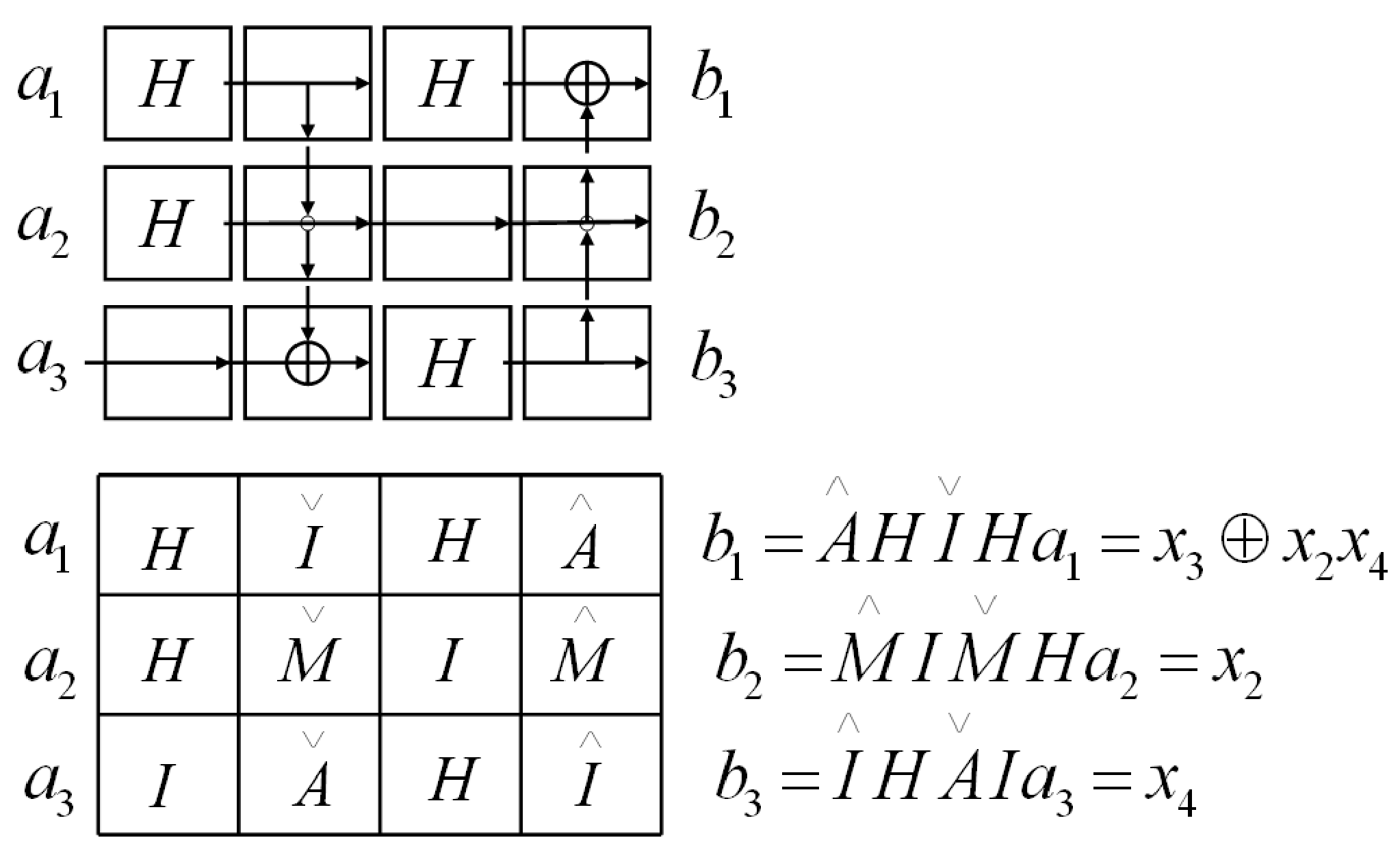
Fig. 1 shows an example of quantum circuit (taken from [1]) and its classical correspondence. The path variables $x_{i}$ comprise the (vector) path $\mathbf{x}=(x_{1},x_{2},x_{3},x_{4})^{T}\in\mathbb{Z}_{2}^{4}$.

A classical path is a sequence of classical bit strings $a,a_{1},a_{2},\ldots,a_{m}=b$ resulting from application of the classical gates. For each selection of values for the path variables $x_{i}$ we have a sequence of classical bit strings which is called an admissible classical path. Each admissible classical path has a phase which is determined by the Hadamard gates applied. The phase is changed only when the input and output of the Hadamard gate are simultaneously equal to 1, and this gives the folmula

Toffoli gates do not change the phase.

For our example the phase of the path $\mathbf{x}$ is

The matrix element of a quantum circuit is given by sum over all the allowed paths from the classical states $\mathbf{a}$ to $\mathbf{b}$

where $h$ is the number of Hadamard gates. The terms in the sum have the same absolute value but vary in sign.

Let $N_{0}$ be the number of positive terms in the sum and $N_{1}$ the number of negative terms

These equations count solutions to a system of $n+1$ polynomials in $h$ variables over $\mathbb{Z}_{2}$. Then the matrix element may be written as the difference

To provide a user with a tool for assembling arbitrary quantum circuits composed from the Hadamard and Toffoli gates we represent a circuit as a rectangular table (Fig. 2).

Each cell in the table contains an elementary gate from following set

so that the output for each row is determined by the composition of the elementary gates in the row. Thereby, each elementary unitary transformation $U_{j}$ is represented as an n-tuple of elementary gates.

Fig. 3 shows action of the elementary gates from (2): the identities, the multiplications, the additions modulo 2, and the classical Hadamard gate. The identity just reproduces its input. The identity-cross reproduces also its vertical input from the top elementary gate to the bottom one and vice versa. Every identity-down and identity-up have two outputs – horizontal and vertical. The multiplication-up and multiplication-down perform multiplication of their horizontal and the corresponding vertical inputs. In a similar manner act the addition-up and addition-down. Each Hadamard gate outputs an independent path variable irrespective of its input and can give a nonzero contribution to the phase.

How can one assemble a circuit? First of all, we define an empty table of the required size. In this case both output and phase are not fixed. Then we place the required elementary gates in appropriate cells. Now the output is the result of applying the elementary gates to the input. The phase is also calculated. Then we proceed the same way with the second column, with the third column, and so on up to the last column. Fig. 4 shows an example.

Apart from the ordinary menu, our program contains the toolbar for selecting an elementary gate and the toolbar for main operations. There are two windows: for assembling a circuit and for showing its polynomials.

A circuit is represented in the program as two $2d$-arrays: one for the elementary gates and another for their polynomials. The phase polynomial is separately represented. The following piece of code demonstrates construction of the circuit polynomials

  for each Column in Table of Gates
    for each Gate in Column {
      construct Gate Polynomial;
      if Gate id Hadamard
        reconstruct Phase Polynomial; }

The method for constructing a gate polynomial is recursive because of the need to go up or down for some gates.

Any circuit is saved as two files. One file is binary and contains the circuit itself. Another file has a text format. It contains the circuit polynomials in a symbolic form. The program allows to save polynomials in several formats convenient for loading into a computer algebra system (for example, in Maple or Mathematica) for the further processing. It is also possible to load back in memory a saved circuit.

Note, that the part of our code for name space Polynomial_Modulo_2 written in C# [4] can also be used independently on our program. This part contains classes for handling polynomials over the finite field $\mathbb{Z}_{2}$. Class Polynomial is a list of monomials, class Monomial is a list of letters, class Letter is an indexed letter provided with a positive integer superscript (power degree).

A system generated by the program is a finite set $F\subset\,R$ of polynomials in the ring

in $h$ variables and $2n$ binary coefficients. One has to count the number of roots $N_{0}$ and $N_{1}$ in $\mathbb{Z}_{2}$ of the polynomial sets

Then the circuit matrix is given by

To count the number of roots one can convert $F_{0}$ and $F_{1}$ into a triangular form by computing the lexicographical Gröbner basis by means of the Buchberger algorithm or by involutive algorithm decribed in [2].

For the example shown on Fig. 1 we have the following polynomial system:

The lexicographical Gröbner basis for the ordering $x_{1}\succ x_{2}\succ x_{3}\succ x_{4}\,\,$ on the variables and representing both $F_{0}$ and $F_{1}$ is as follows

From this lexicographical Gröbner basis we immediately obtain the following conditions on the parameters:

From these conditions we easily count 2 (0) roots of $F_{0}$ ($F_{1}$) and 0 (2) roots of $F_{0}$ ($F_{1}$). In all other cases there is 1 root of $F_{0}$ and $F_{1}$.

Some matrix elements are

We presented the first version of a program tool for assembling arbitrary quantum circuits and for constructing the corresponding polynomial equation systems. Its number of solutions uniquely determines the circuit matrix.

There is the algorithmic Gröbner basis approach to converting the system of quantum polynomials into a triangular form which is useful for computing the number of solutions.

Thus, the above presented software together with Gröbner bases provide a tool for simulating quantum circuits.

The research presented in this paper was partially supported by the grant 04-01-00784 from the Russian Foundation for Basic Research.

References

- [1] Christopher M. Dawson et al. Quantum computing and polynomial equations over the finite field . arXiv:quant-ph/0408129.
- [2] Gerdt V.P. Involutive Algorithms for Computing Grobner Bases. Computational commutative and non-commutative algebraic geometry, IOS Press, Amsterdam, 2005, pp.199-225. arXiv:math.AC/0501111, 2005.
- [3] Aharonov D. A Simple Proof that Toffoli and Hadamard Gatesare Quantum Universal. arXiv:quant-ph/0301040.
- [4] Microsoft Visual C# .net Standard, Version 2003.