Quantum and classical correlations of intense beams of light via joint photodetection
Abstract
We address joint photodetection as a method to discriminate between the classical correlations of a thermal beam divided by a beam splitter and the quantum entanglement of a twin-beam obtained by parametric downconversion. We show that for intense beams of light the detection of the difference photocurrent may be used, in principle, in order to reveal entanglement, while the simple measurement of the correlation coefficient is not sufficient. We have experimentally measured the correlation coefficient and the variance of the difference photocurrent on several classical and quantum states. Results are in good agreement with theoretical predictions taking into account the extra noise in the generated fields that is due to the pump-laser fluctuations.
1 Introduction
Entanglement is a crucial resource in quantum information processing, quantum communication and quantum measurements. Indeed quantum correlations lead to important novel effects not achievable by using classically-correlated states, i.e. states characterized by correlations that may be established by using local operations and classical communication. Quantum information has been initially developed for discrete quantum variables, i.e. quantum bits, which can be implemented optically by means of polarization single-photon states. However, much attention has been recently devoted to continuous variable (CV) regime and to multiphoton states of light. Continuous-spectrum quantum variables may be easier to manipulate compared to quantum bits by means of linear optical circuits and homodyne detection [1, 2, 3]: this is the case of Gaussian states of light, e.g. squeezed- and twin-beam. By using CV one may carry out nonlocality experiments [4], quantum teleportation [5] and generation of multimode entanglement [6]. The concepts of quantum cloning [7] and entanglement purification [8] have also been extended to CV, and secure quantum communication protocols have been proposed [9].
Ideal features for implementing quantum information experiments are the availability of bright and stable entanglement sources, based on degenerate or nondegenerate optical parametric processes, and the possibility of an effective characterization of entanglement. In the case of CV Gaussian entanglement quantum correlations may be discriminated from classical correlations by using homodyne detection. However, homodyne detection requires an appropriate mode matching of the signals with a local oscillator at a beam splitter, a task that may be particularly challenging in the case of pulsed optical fields. On/off photodetection may be also used to characterize Gaussian states, but its use is limited to states with a small number of photons [10, 11].
For the reasons of above, in this paper we assess the use of intensity measurements, in particular joint photodetection, as a method to discriminate classical correlations from entanglement [12]. A simple intensity-based measurement, including the measurement of difference photocurrent, cannot provide a complete characterization of entanglement. However, we show that for intense beams of light the detection of the difference photocurrent may be used, in principle, in order to reveal entanglement, while the simple measurement of the correlation coefficient is not sufficient. In particular, joint photodetection can be useful to discriminate the entanglement of twin-beam from correlations of thermal sources in the mesoscopic regime. We have experimentally measured the correlation coefficient and the variance of the difference photocurrent on several classical and quantum states. Results are in good agreement with theoretical predictions if one takes into account the extra noise in the generated states caused by the pump laser fluctuations.
This work may also contribute to the recent debate on the use of classical and quantum correlations in imaging and on the necessity of entanglement for extracting the information [13]. Our results indicate that any method only based on correlation measurements cannot be improved using entanglement instead of classical correlations.
The paper is structured as follows. In Section 2 we theoretically analyze the joint photodetection of classically and quantum correlated fields. In section 3 we present the experimental results obtained for a quantum (twin beam) and a classical (thermal light divided by a beam splitter) light. In Section 4 we discuss the experimental results and draw our conclusions in Section 5.
2 Quantum versus classical correlations
Our aim is to assess the use of joint photodetection as a method to discriminate classical correlations from entanglement. The scheme we are going to consider is the following: two modes of radiation, say and , are independently measured by two photodiodes, and the resulting photocurrents and are then electronically manipulated and analyzed. In the following we first investigate the use of the correlation function as an entanglement marker, and then pass to consider the difference photocurrent, of which we analyze both the variance and the distribution as a whole. The different markers are compared in order to discriminate entangled twin-beam (TWB) of radiation from i) a two-mode factorized coherent state showing no correlations, and ii) a two-mode thermal beam, showing classical correlations only. Since entanglement of TWB is a monotone function of its energy the comparison are performed for fixed mean number of photons of the involved signals.
Entangled twin-beam are obtained in quantum optics from (spontaneous) parametric downconversion (SPDC) in second order nonlinear crystals. The expression in the number basis is given by
| (1) |
where denotes a Fock number state in the Hilbert space of the -th mode. The parameter satisfies and may be taken as real without loss of generality. The value of depends on the crystal length and on the nonlinear susceptibility, whereas the mean photon number of the TWB is given by , where with , and is the mean photon number of each beam. As a benchmark for uncorrelated classical signals we consider a two-mode coherent state of the same energy of the TWB, i.e. with . On the other hand, as a reference for classically correlated signals we consider the state obtained by sending a thermal state on a balanced beam-splitter whose second port is left unexcited. In general, if we mix a quantum state with the vacuum in a beam-splitter of transmissivity , the outgoing state is described by the density matrix
where are the matrix elements of the input state. In our case and the input state is a thermal state with mean photon number, i.e with . We will denote the state obtained in this way as . As it can be easily seen by evaluating the eigenvalues of the partial transpose , the state exiting a beam-splitter fed by a thermal state is never entangled, though it may show a high degree of classical correlations.
We assume that photodetection is performed with quantum efficiency and no dark counts. The probability operator-valued measure (POVM) of each detector, describing the statistics of detected photons, is thus given by a Bernoullian convolution of the ideal number operator spectral measure
with . The joint distribution of detected photons can be evaluated by tracing over the density matrix of the two modes, i.e. while the moments of the distribution are evaluated by means of the operators
| (10) |
where
Of course, since they are operatorial moments of a POVM, we have, in general, . The first two moments correspond to the operators
| (14) |
As a consequence, the variances of the two photocurrents are larger than the corresponding photon number variances. We have
| (15) |
The correlation coefficient is defined as
| (16) |
where and are given in Eqs. (14) and (15) respectively. Of course, for factorized coherent states we have , while for the TWB and the thermal states we have
| (17) |
which, for reduce to
| (18) |
As it is apparent from Eqs. (17) and (18) the correlation coefficient cannot provide a reliable discrimination of classical and quantum correlations for a mean number of photons larger than few units. As a consequence, any imaging system based on coincidence detection, cannot be improved by using entanglement.
Let us now consider the quantity obtained by subtracting the two photocurrents from each other, i.e. the so-called difference photocurrent . The statistics of the outcome can be obtained as where the POVM is given by
with given in Eq. (2). The moments of the distribution can be obtained from the operators
| (23) |
| (24) |
which also provide the variance of the difference photocurrent . For the class of states under investigation the difference photocurrent is distributed as follows
| (25) | |||
| (31) | |||
| (35) |
where denotes a modified Bessel’ function of the first kind, and the quantities are given by
In Equation (35) the sum are over , or and over , otherwise. The distributions are symmetric for and asymmetric otherwise. In Fig. 1 we display the distributions , , and for different values of the parameters , and . As it is apparent from the plots, the distributions for a thermal or a coherent state are broader than for the TWB, as far as the quantum efficiencies are close to each other and their value is not too small. In order to quantify this statement more explicitly we have evaluated, by using Eqs. (23) and (24), the variance of the difference photocurrent for the three types of states. We have
| (52) | |||||
| (53) | |||||
| (54) |
For the variances for the two classical states are equal, and larger than for the TWB state: the difference being more pronounced the greater is the value. On the other hand, if the two quantum efficiencies are different, we have and for any value of the mean photon number , whereas only for numbers of photon below the threshold value
| (55) |
In other words, for equal quantum efficiencies the variance of the difference photocurrent is a good marker to discriminate between quantum and classical correlations, whereas for different quantum efficiencies this statement is true only for signals with a small number of photons. In Figs. 2 we report the variances as a function of the mean number of photons for both and , whereas in Fig. 3 we show for as a function of .
Let us now consider a situation in which the two beams under investigation contain more than two, say , modes of the field, while the correlations to be discriminated are still pairwise. This is a common situation in pulsed experiments where several temporal modes are simultaneously matched in SPDC, and are present in thermal beams as well. We assume that the modes are equally populated. The statistics of counts for each detector is described by a multimode POVM of the form
| (56) |
where is the single-mode POVM reported in Eq. (2). The statistics of the difference photocurrent between the two detectors is described by a -mode POVM of the form (2), with replaced by .
Since the modes entering each detector are independent on each other we have and , . As a consequence the expressions of the correlation coefficients are still given by Eqs. (17) with that should be meant as the total mean number of photons of the modes. As concerns the distribution of the difference photocurrent we have, in terms of the probability density
| (57) | |||||
where is the Heaviside step function. Notice that in writing Eq. (57), we have already used the fact that the correlations are pairwise i.e. that . By exploiting the delta functions in (57) we may write
| (58) | |||||
for and an analogue expression (with ) for .
3 Experimentals
We verified the validity of the theoretical analysis on both quantum and classically correlated light.
3.1 Twin Beam
The quantum state of light we consider is a pulsed twin-beam generated by a traveling-wave amplifier in non-degenerate configuration. The layout of the experiment is depicted in Fig. 4. As the pump source we use a frequency-tripled continuous-wave mode-locked Nd:YLF laser regeneratively amplified at a repetition rate of 500 Hz (High Q Laser Production, Hohenems, Austria). The laser delivers 7.7 ps pulses at the fundamental frequency and 4.5 ps pulses at the third harmonics. We obtain intense spontaneous parametric generation in broadly tunable cones by injecting the pump field () into an uncoated -BaB2O4 crystal (BBO, Fujian Castech Crystals, Fuzhou, China) cut for type I interaction (cut angle: 34 deg) having mm2 cross-section and 4 mm thickness. The pump beam, which emerges from the laser slightly divergent, is focused by lens of 50 cm focal length. The crystal tuning angle is and the visible portion of the cones projected on a screen beyond the BBO is shown in the inset of Fig. 4. We operate in a dichromatic configuration by choosing the frequency of the laser second harmonics () for the signal and consequently the frequency of the laser fundamental () for the idler. For alignment purposes, a portion of the fundamental beam emerging from the laser is injected in the crystal together with the pump beam so as to obtain a well recognizable spot of amplified seeded down conversion. The selection of the two components of the twin beam is performed by means of two pin-holes, and , having suitable dimensions, located on the outputs of the seeded process. In order to decide the dimensions of the pin-holes, such to collect a single coherence area at a time, we have to determine the dimensions of the coherence areas of the generated fields. In Fig. 5 (left) we show the single-shot picture of a portion of the signal cone taken with a digital camera (model Coolpix 990, Nikon, resolution ), in which we can clearly distinguish the presence of the coherence areas. In the right part (top) of the same figure we show a magnified single coherence area around (green light) and (bottom) the intensity map of a typical coherence area taken with a CCD camera (model TM-6CN, Pulnix, operated at high-resolution). It is easy to demonstrate that the dimensions of the coherence areas in the idler beam (IR) corresponding to the measured signal beam scale according to the ratio of the involved wavelengths so that the dimensions for the idler are doubled with respect to the signal [14]. Accordingly, as shown in Fig. 4, to select a single coherence area on signal and idler, we locate two pin-holes (diameter , on the signal and diameter , on the idler) at a distance of from BBO. The light selected by the pin-holes is then focused with two lenses ( and , focal length 25 mm) on two p-i-n photodiodes (Si 85973-02 Hamamatsu, 1 ns time-response, 500 m diameter sensitive area on the green and InGaAs G8376-05, Hamamatsu, 5 ns time-response, 500 m diameter sensitive area on the IR) having nominal quantum efficiencies and respectively. The current outputs of the photodiodes are integrated over a synchronous gate of suitable time duration (40 ns) by a boxcar averager that is operated as gated integrator in external trigger modality. The boxcar output is digitized by a 13-bit converter (SR250, Stanford Research Systems, with 50 mV full-scale) and the counts stored in a PC based multi channel analyzer (MCA). The measurements are performed by inserting a variable filter ( in the figure) in front of the photodiode detecting the signal, and by carefully adjusting it to balance the quantum efficiencies of the two detection branches of the setup. The interpretation of the output data must take into account the presence of cut-off filters, inserted to eliminate residual pump and all stray light, the overall quantum efficiency of the detection apparatus results to be . We verify the linearity of the boxcar integrators and measure the conversion coefficients ( and ) by linking the voltage output of the digitizer to the number of electrons forming the photocurrent output pulse of the detectors at each laser shot. The relations among the statistics of the number of photons incident on the detector, , the statistics of the number of detected photons, , and the statistics of the output voltages of the acquisition apparatus, , are given by
| (62) |
being the measured conversion coefficient mentioned above and a normalization coefficient. If we limit our analysis to the first two moments of the distributions, the experimental outputs are linked to Eq.s (14) and (15) by
| (63) | |||
| (64) |
where for the sake of clarity we have defined and [see Eq. (15)]. Note that in general the statistical distribution for the measured outputs is different from that of the incident photons. However, in both our cases (quantum and classical), the statistical distributions of the detected photons and of the voltage outputs are thermal ones.
In Fig. 6 we show the recorded signal (left) and idler (right) outputs of the photodiodes as a function of the laser shot, together with the noise of the detectors. In Fig. 7 we the corresponding normalized probability distributions are reported for the same data. By looking at the probability distributions in Fig. 7 we note that the statistics of the outputs are well fitted by multithermal distributions [15], that is the distributions obtained by the convolution of equally populated thermal modes
| (65) |
where is the mean output corresponding to the overall detected photons mean value . Equation (65) holds in the high-intensity regime, which is the present experimental condition. In fact, by using the measured conversion coefficients on the detection arms of signal and idler we get and as the mean number of detected photons. As it is well known from the theory of photodetection [16], the number of detected modes can be interpreted as the ratio of the time characteristic of the measurement (in our case the time duration of the pulse) and the coherence time characteristic of the field to be measured (in our case the inverse of the temporal bandwidth of the spontaneous parametric down conversion) [15]. The continuous lines superimposed to the histograms of the experimental data in Fig. 7 show the convolution integrals, optimized for the number of temporal modes, of the theoretical distribution in Eq. (65) with the system impulse response evaluated from a measure in the absence of incident light. As expected, the signal and idler distributions are well fitted by multithermal distributions having the same number of modes (). Note that the probability distributions for signal and idler are very similar to each other. In order to stress the correspondence between signal and idler, we plot the output of the idler as a function of that of the signal (see Inset in Fig. 8). To compare the experimental results with the theoretical predictions, we first of evaluate the correlation function of the photocurrents as
| (66) |
where the average operations are taken over (typically ) subsequent laser shots. For , Eq. (66) gives the correlation coefficient
| (67) |
which should be compared with the theoretical predictions of Eqs.(17) and (18). In Fig. 8 we show the correlation coefficient for the data of Figs. 6 and 7: the contributions of the noise of the apparatus, (i.e. the variance of the impulse response in Fig. 7), are subtracted from the measured variances of the experimental data. We get , to be compared with a theoretical value of about . Note that subsequent shots results to be uncorrelated.
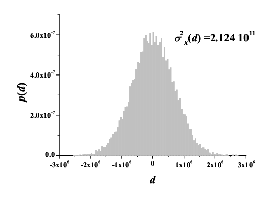
As it has been shown in Section 2, the distribution of the difference photocurrent is a relevant marker of entanglement. In Fig. 9 we plot the distribution of the difference of the photoelectrons detected on signal and idler, i.e. . The distribution appears almost symmetrical and centered at zero, which indicates both accurate balance of the detectors’ quantum efficiencies and high correlation in signal/idler photon numbers. The variance, as evaluated from the data, once the variance of the noise is subtracted, turns out to be .
3.2 Thermal Light
To investigate joint photodetection for classically correlated light, we modify the experimental setup according to Fig. 10. Pseudo-thermal light has been generated by inserting a moving ground-glass diffusing plate in the path of the second-harmonics output of the laser ( nm). A portion of diffused light is selected with an iris (in Fig. 10) and then sent to a 50 cube beam splitter. The temporal statistics of the generated light can be described by the same statistics as in Eq. 65 [17], in which the number of modes can be varied by changing the dimension of the iris in order to collect more than one spatial coherence area. The beams emerging from the beam splitter are then detected by the same apparatus used for the twin beam, where the pin photodiodes are now identical (model S3883-02, Hamamatsu, , nominal) since the two beams are at the same frequency. The mean number of detected photons on the two beams are .
In Fig. 11 we show the normalized probability distributions for the detected photons. The continuous lines superimposed to experimental data in Fig. 11 are the best fits of the data obtained for 15 modes. As in the case of the twin beam, the two histograms are very similar and suggest a high degree of correlation that is easily verified evaluating the value of the correlation function. In the Inset of Fig. 12, we plot the two voltage outputs of the beam splitter one versus the other, and in right part the correlation function for the classical beams in which again the contributions of the noise of the apparatus have been subtracted from the measured variances of the experimental data. We get to be compared with a theoretical value of about .
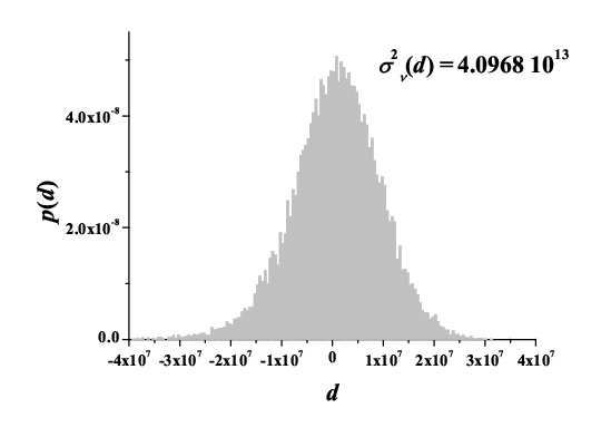
In Fig. 13 we plot the distribution of the difference of the photoelectrons detected on the two arms of the beam splitter. Again the distribution appears symmetrical and peaking at zero. The variance, as evaluated from the data upon subtraction of the noise, is .
4 Discussion
The experimental results discussed in Section 3 are obtained by keeping the values of the quantum efficiencies as close each other as possible. Therefore, they must be compared with the expected values for equal quantum efficiencies and with the shot-noise level for the intensities we are working at. The theoretical values are and for the TWB and for the classically correlated thermal light. In order to obtain a realistic comparison between theory and experiment, we have to take into account the presence of noise that unavoidably affects the experimental data. We identify two main sources of noise: first of all, the difference between the overall quantum efficiencies on the two detection branches. In fact, although the experimental procedure was optimized so as to obtain the best balanced values, a small residual difference cannot be excluded, and, as we will see, a small balance error, even local across the beam to be measured, produces a relevant difference in the values of . On the other hand, we have to take into account the unavoidable fluctuations of the laser source which affect all the fields under investigation. In fact, the pulsed pump field is not a plane wave having constant amplitude. Rather, its statistics is more realistically modeled by a Gaussian distribution, i.e. a Poissonian distribution affected by an excess noise [18]
| (68) |
where and is the increase of the variance due to fluctuations; the quantity measures the amount of such a deviation. We will evaluate the influence on the generated beams of the excess noise in the pump by evaluating the error propagation.
4.1 Imbalance of the quantum efficiencies
To evaluate the modifications of the experimental results due to imbalance in the quantum efficiencies of the two branches, we equate the experimental results for with the theoretical predictions for unbalanced quantum efficiencies of the photodetectors (see Eqs. (53) and (54) for ). In the case of TWB, we obtain and in the case of classical field . These values are too large to be reconciled with the high symmetry of the measured (see Fig. 13). We can thus conclude that simply including a difference in the quantum efficiencies on the two detection branches is not sufficient to account for the experimental data.
4.2 Fluctuations in the laser source
We evaluate the influence of the excess noise of the third-harmonics pump pulse on the generated beams.
Starting with the SPDC, we recall that the mean photon number in each component of the generated twin beam is given by
| (69) |
where is a coupling constant, is the interaction length inside the crystal and , being the mean photon number, the cross section and the temporal duration of the pump pulse. By applying the error-propagation theory to Eq. (69), we get for the excess noise in the single mode of signal (idler):
| (70) | |||||
where we used Eq. (69) and the final approximation holds for . In the case of a multithermal beam composed by modes, Eq. (70) becomes:
| (71) |
The variance of the difference photocurrent can thus be corrected as
| (72) |
which is a function of the parameter . We now evaluate the amount of laser fluctuations (i.e. the value of ) needed to reproduce the experimental data. To this aim, we equate Eq. (72) to Eq. (54), modified to consider the presence of modes in the measured field
| (73) |
and study the dependence of on the value of the overall quantum efficiencies on the two detected fields. Notice that, from the experimental point of view, we have two possible choices for the value of appearing in the theoretical formula, namely with indicating either signal or idler, in our experimental conditions and the two conditions give very similar results. Figure 14 displays the values of as a function of and (left), and the corresponding values of the corrected as calculated from Eq. (72) (right). The horizontal plane in on the right represents the shot-noise level of the measure as calculated from Eq. (52). Starting from data in Fig. 14 we can draw two conclusions: On one hand, the experimental data corresponds to an amount of laser excess noise equal to , which is compatible with the fluctuations of a pulsed laser. On the other hand, we have that at the intensities used in our experiments we cannot reliably discriminate the measured from the shot-noise level. In fact, the right part of Fig. 14 shows that a slight indetermination in the quantum efficiencies may considerably increase the variance above the shot noise level. Note that the inclusion of an added noise does not imply a significant modification of the variance of the beams, as the total variance of signal/idler can be written as
| (74) |
As the correction to unity is less than , the measured distributions are still well fitted by the expected multithermal distributions.
As concerning the thermal light experiments, by applying the same strategy, we find that the excess noise can be written as
| (75) |
which is again a function of the laser fluctuations . Again we equate the value of the measured corrected for the added noise and study the dependence of on and . Figure 15 displays the values of as a function of and (left), and the corresponding values of the corrected (right). The horizontal plane on the right represents the shot-noise level of the measure as calculated from Eq. (52). The highest values of the laser fluctuations, which are found for , is at most. In contrast with the case of the TWB, from Fig. 15 we see that the values of are always above the horizontal plane representing the shot-noise level of the measure.
In order to check the plausibility of the calculated values of , we perform a stability measurements on the laser, by simultaneously detecting the second- and third-harmonics outputs of the laser with two photodiodes. In Fig. 16 we plot the measured values of as a function of the third-harmonics energy in arbitrary units. The marked energy intervals in the plot indicate the operating range of the measurements discussed above. The obtained values of are in agreement with those calculated.
5 Conclusion
Establishing the existence of entanglement and discriminating between classically and quantum correlated states in the high-intensity continuous-variable regime is a challenging task motivated by the need of characterizing the nature of the correlated light and of understanding the real resources needed to achieve the results in specific situations. We demonstrate that the characterization in terms of correlation functions is not satisfactory, as it gives similar results in both classical and quantum domain, whereas the measurement of the probability distribution for the difference photocurrent is in principle a good strategy. On the other hand, we demonstrate that in realistic high intensity conditions such a strategy cannot be reliably adopted, due to the unavoidable fluctuations of the laser source and slight imbalance of the detectors’ quantum efficiencies. Indeed, by correcting the experimental data for these sources of noise, the data analysis leads to an agreement with the expected results.
To achieve a more direct experimental demonstration we can follow two strategies. On one hand, we could work with identical quantum efficiencies, i.e. at frequency degeneracy, and use the same detection system on both parties of the correlated state. This could be done, for instance, by substituting the p-i-n photodiodes with a CCD camera. On the other hand, one may lower the intensity of the field to be measured, to decrease the sensitivity to the excess noise due to the pumping laser. Notice that, however, the possibility of lowering the intensity is limited by the amplifying capability of the electronic chain that manipulates the photodiode outputs. To overcome this limitation, one should switch to detectors with internal gain, such as photomultiplier tubes and hybrid photodetectors, taking into account that these detectors shows a low quantum efficiency of the photoelectric emission of the photocathodes which may compromises the overall visibility.
In conclusion we have shown that difference photocurrent may be used, in principle, in order to reveal entanglement, while the simple measurement of the correlation coefficient is not sufficient. Our experimental results indicate that joint photodetection may be useful to discriminate the entanglement of twin-beam from correlations of thermal sources in the mesoscopic regime.
Acknowledgments
This work has been supported by MIUR (FIRB RBAU014CLC-002) and by INFM (PRA-CLON). The Authors thanks F. Ferri for stimulating discussion on the statistics of thermal light and E. Gevinti, P. Rindi, E. Puddu and G. Zambra for technical support during the measurements.
References
References
- [1] See for example, Quantum Information Theory with Continuous Variables, S.L.Braunstein and A.K.Pati Eds (Kluwer, 2002).
- [2] A. Ferraro, S. Olivares and M. G. A. Paris, “Gaussian States in Quantum Information ”, Napoli Series on Physics and Astrophysics (Bibliopolis, Napoli, 2005); e-print, quant-ph/0503237.
- [3] E. Knill, R. Laflamme, and G. J. Milburn, Nature 409, 46 (2001); U. L. Andersen, V. Josse and G. Leuchs, e-print quant-ph/0501005.
- [4] K. Banaszek, and K. Wódkiewicz, Phys. Rev. Lett. 82, 2009 (1999); K. Banaszek, A. Dragan, K. Wódkiewicz, and C. Radzewicz Phys. Rev. A 66, 043803 (2002).
- [5] A. Furusawa et al, Science 282, 706 (1998).
- [6] J. Jing et al., Phys. Rev. Lett. 90, 167903 (2003); T. Aoki et al., Phys. Rev. Lett. 91, 080404 (2003); H. Yonezawa, T. Aoki and A. Furusawa, Nature 431, 430 (2004); R. C. Pooser and O. Pfister, e-print, quant-ph/0505130; M. Bondani et al., Opt. Lett. 29, 180 (2004).
- [7] P. van Loock, and S. Braunstein, Phys. Rev. Lett. 87, (2001); S.L. Braunstein, et al, Phys. Rev. A 63, 052313 (2001); N. Cerf, J. Mod. Opt. 47, 187 (2000); N. Cerf, A. Ipe, X. Rottenberg, Phys. Rev. Lett. 85, 1754 (2000); S. L. Braunstein et al, Phys. Rev. Lett. 86, 4938 (2001); N. Cerf et al, Eur. Phys. J. D 18, 211 (2002). A. Ferraro, M. G. A. Paris, A. Allevi, A. Andreoni, M. Bondani, E. Puddu, J. Opt. Soc. Am. B 21, 1241 (2004).
- [8] L. Duan, G. Giedke, J. I. Cirac, and P. Zoller, Phys. Rev. Lett. 84, 4002 (2000).
- [9] F. Grosshans, P. Grangier, Phys. Rev. Lett. 88, 057902 (2002)
- [10] J. Fiurasek, N. Cerf, Phys. Rev. Lett. 93, 063601 (2004).
- [11] G. Zambra et al, Phys. Rev. Lett. 95, (2005).
- [12] D. T. Smithey et al, Phys. Rev. Lett. 69, 2650 (1992).
- [13] B. E. A. Saleh, A. F. Abouraddy, A. V. Sergienko, and M. C. Teich, Phys. Rev. A 62, 043816 (2000); A. F. Abouraddy, B. E. A. Saleh, A. V. Sergienko, and M. C. Teich, Phys. Rev. Lett. 87, 123602 (2001); A. F. Abouraddy, B. E. A. Saleh, A. V. Sergienko, and M. C. Teich, J. Opt. Soc. Am. B 19, 11741184 (2002); A. Gatti, E. Brambilla, and L. A. Lugiato, Phys. Rev. Lett. 90, 133603 (2003); A. Gatti, E. Brambilla, M. Bache, and L. A. Lugiato, Phys. Rev. Lett. 93, 093602 (2004).
- [14] A. Agliati, A. Allevi, M. Bondani, E. Gevinti, P. Rindi, and A. Andreoni, Spatial coherence areas in Spontaneous Parametric Downconversion, manuscript in preparation.
- [15] F. Paleari, A. Andreoni, G. Zambra, and M. Bondani, Opt. Express 12, 2816-2824 (2004).
- [16] L. Mandel and E. Wolf, Optical Coherence and Quantum Optics (Cambridge University Press, Cambridge, 1995), chapter 14.
- [17] J. W. Goodman, Statistical Optics (John Wiley & Sons, New York, 1985), chapter 2.
- [18] R. Loudon, The Quantum Theory of Light, (Oxford University Press, New York, 2000).