Classical capacity of fermionic product channels
Abstract
We study multi-qubit quantum channels that can be represented as a product of one-mode fermionic attenuation channels. An explicit formula for the classical capacity and for the minimum output entropy of these channels is proposed. We compute analytically for any number of qubits under assumption that the minimum is achieved on a Gaussian input. Apart from that, a simple numerical method for evaluating is developed. The method is applicable to any channels that are sufficiently noisy. For fermionic product channels the proposed formula for agrees with the numerical results with a precision about .
I Introduction and summary of results
Transmission of a classical information through a quantum communication channel is one of the basic problems studied in the quantum information theory. Suppose a sender (Alice) wants to send a string of classical bits through a one-way noisy quantum channel to a receiver (Bob). Suppose Alice is allowed to use the channel only times. A number is called an achievable rate if for any there exists a transmission protocol with and an error probability smaller than . The classical capacity of is defined as the minimum number such that for any achievable rate . A closely related quantity is a one-shot capacity which is defined analogously to with a restriction that Alice uses only product states for signaling. It has been shown that and conjectured that actually , i.e., is additive under tensor product of channels. The Holevo-Schumacher-Westmoreland theorem SW97; Holevo98 states that
| (1) |
where is a probabilistic ensemble of states from the image of (a set of all output states), and is the Holevo quantity
| (2) |
Important examples of quantum channels for which an explicit formula for the classical capacity is known are product of one-qubit unital channels King02 and products of bosonic attenuation channels MIT04. In the latter case a restriction on a power of the input signal has to be imposed to regularize the capacity. An explicit formula for the one-shot capacity is also conjectured for bosonic attenuation channels combined with a classical Gaussian noise HW01.
Quantum channels explored in this paper are direct fermionic analogues of bosonic product channels studied in MIT04. In contrast to their bosonic counterparts, fermionic modes are described by a finite-dimensional Hilbert space, so one does not need to regularize the capacity.
An algebra of observables of fermionic modes formally coincides with the one of qubits and can be conveniently described by generators ,
| (3) |
Here are the Pauli operators on the qubit . This is the well-known Jordan-Wigner transformation that is often used to map a system of spins (qubits) into a system of fermions. The generators obey the Clifford algebra commutation rules
An arbitrary linear operator acting on qubits can be uniquely represented as a linear combination of monomials
where is a binary string of bits.
Define a quantum channel by the following rules
| (4) |
Here are real parameters specifying the channel (attenuation coefficients). A proof that the linear map defined in Eq. (I) is indeed a quantum channel (i.e. a trace preserving completely positive map) as well as some motivation of this definition will be given in Section II. It suffices to mention now that has a clear product structure. One can say that the system of qubits is ‘partitioned’ into separated subsystems (Majorana fermionic modes) that are described by the operators . Each subsystem is transmitted independently through its own ‘wire’ described by a quantum channel . However this product structure should not be mixed with the tensor product of quantum channels. Indeed, we shall see in Section II that Krauss operators corresponding to different ‘wires’ do not commute. Accordingly, one can not expect that the capacity of the channel Eq. (I) will be additive (a capacity of an individual wire is not even a well-defined quantity).
To compute the maximum at Eq. (1) we shall use a certain variational family of states, namely, fermionic Gaussian states TD02; Bravyi05. A Gaussian state is completely specified by its first and second moments , , see Section III for a strict definition. In particular, the von Neumann entropy is a simple function of these moments. We will see that the product fermionic channels map Gaussian states into Gaussian states. Define a Gaussian capacity as
| (5) |
where is an ensemble of Gaussian states (probabilities may be arbitrary though). This is the best transmission rate that can be achieved if Alice uses only product Gaussian states for signalling. Obviously, . Our main result is an explicit formula for the Gaussian capacity.
Theorem 1.
Let be a fermionic product channel acting on qubits with attenuation coefficients . Denote the -largest coefficient. Then
| (6) |
where is the Shannon binary entropy. Moreover, if .
A proof of the theorem as well as some additional results that are valid for Gaussian input states is given in Section IV.
The theorem implies that the optimal signaling ensemble is Gaussian for . Can one achieve a higher transmission rate for by using non-Gaussian ensembles? To get some intuition about it, we have tried to calculate numerically for three and four qubits, see Section V. The numerical results strongly suggest that , i.e., that we gain nothing from using non-Gaussian signaling states. It might seem rather surprising because mixed Gaussian states are known to be the maximally noisy states (in terms of their von Neumann entropy) for fixed first and second moments. On the other hand, one can easily see from Eq. (I) that the channel washes out correlations among large number of modes such that -mode correlators acquire a factor , where is a typical value of . It means that two-mode correlations is the best place to keep the information that has to be sent through the channel. In this respect Gaussian states are very promising candidates, because they have only two-mode correlations. Therefore, there might be a subtle tradeoff between large entropy of Gaussian states and their special correlation structure that makes them optimal for signaling.
In general, a computation of (even numerical) is an extremely hard problem. Fortunately, the fermionic product channels possess a special symmetry property known as covariance, see Holevo02; Cortese02. For covariant -qubit channels the one-shot capacity is given by
| (7) |
where
| (8) |
is the minimum output entropy. Our derivation of the Gaussian capacity is actually a computation of the minimum output entropy for Gaussian input states. The analogous problem has been already solved for bosonic Gaussian channels MIT03 and a conjecture has been made that the global minimum of the output entropy is achieved on a Gaussian input. Whether or not this conjecture is true in the fermionic world is an open question (which is equivalent to an equality ).
In Section V we describe a simple algorithm that allows one to evaluate for many quantum channels. Applicability of the algorithm is not restricted to the fermionic product channels. In general, the algorithm works well if is not too close to an ideal channel. The main idea is to exploit positivity of the relative entropy and iteratively minimize . More specifically, we construct a sequence of pure states , such that is the largest eigenvector of an operator . The initial state is chosen randomly. One can easily show that , i.e., the corresponding sequence of output entropies is non-increasing. One should repeat the iterations until the output entropy keeps decreasing.
In contrast to local search methods, such as the gradient descent, the iterative minimization is able to escape from local minimums of the objective function. However, one can not guarantee that the iterations converge to the global minimum, see Section V for more detailed discussion.
In Section V.B we use the algorithm to find the minimum output entropy of the fermionic product channels for three-qubit and four-qubit systems. The corresponding value of the capacity matches the Gaussian capacity with a precision about which has the same order of magnitude as the numerical noise. It is therefore fair to make a conjecture that in general.
The rest of the paper is organized as follows. Section II contains all the necessary facts about fermionic product channels. In Section III we review some basic properties of Gaussian states. Computation of the minimal output entropy for Gaussian input is done in Section IV. Also in this section we show that the image of a fermionic product channel has a nicely ordered structure with respect to the majorization relation. The algorithm for computation of the minimal output entropy and the numerical results obtained with its help are discussed in Section V.
II Basic properties of the fermionic product channel
II.1 Krauss representation
We start from constructing an explicit Krauss representation for the channel defined in Eq. (I). Consider a parity generator
| (9) |
In terms of qubits it looks as . One can easily check that
where is the Hamming weight of the string . Introduce Krauss operators
A one-mode quantum channel
implements the transformation Eq. (I) with for all . Note that is a trace preserving completely positive (TPCP) map iff . Since the one-mode channels commute, , we conclude that
| (10) |
Accordingly, is a TPCP map for all . Expanding the product Eq. (10) yields the desired Krauss representation of ,
| (11) |
where
The channels related by a transformation for some are unitarily equivalent, so we can focus on non-negative values .
II.2 Covariance
The subsection summurazes some ideas proposed in the papers Holevo02; Cortese02. Let be a set of -qubit unitary operators (which may or may not constitute a group) that completely randomize any quantum state:
| (12) |
A quantum channel is said to be covariant if it commutes with all operators , i.e.,
for any operator . Covariance is a very useful property of a channel that allows one to reduce the problem of calculating the capacity to the problem of finding the minimum output entropy of a channel, see Eq. (8). Indeed, let be a state with the minimum output entropy. Consider an esemble of pure states , where is chosen randomly and uniformly from the set . This ensemble has the maximally mixed average state since . Therefore the Holevo quantity of this ensemble is . Obviously, this is the absolute maximum of the Holevo quantity for any ensemble of states in , so that for any covariant channel.
The channel defined in Eq. (I) is covariant. Indeed, let be the set of operators . One can easily check that
It means that possesses the randomizing property Eq. (12). On the other hand it is obvious that
for any operator . Therefore is covariant channel, and its one-shot capacity can be found from Eq. (7).
II.3 Physical motivation
Under certain circumstances the fermionic product channels may adequately describe evolution of fermi systems interacting with environment. As a toy model consider a fermi system that consists of a single fermionic mode () which we describe by creation/annihilation operators , . Suppose the system interacts with an environment which also can be described by a single fermionic mode , . Suppose the interaction between the system and the environment is just the hopping Hamiltonian . We assume that the initial state of the environment is maximaly mixed, . The toy model channel is defined as
After straighforward calculations one gets
where . Introducing generators , we get: and . This is an example of the product fermionic channel Eq. (I) with and . More generally, if the environment possesses a superconducting order parameter, the interaction Hamiltonian may include terms with particle-hole conversion, like in Andreev reflection of electrons. In this case one can tune the interaction to obtain an arbitrary string of coefficients .
III Gaussian states of fermions
In this section we describe a variational family of -qubit states that will be used to minimize the output entropy of the channel Eq. (I). These are Gaussian states. The simplest example of a Gaussian state is the Fock vacuum or any other product state diagonal in the standard basis. Denote
| (13) |
An arbitrary Gaussian state can be converted into the standard form by a unitary evolution with a Hamiltonian quadratic in the operators . Here is a strict definition.
Definition 1.
A state is Gaussian iff it can be represented as
| (14) |
where and are Hermitian linear combinations of operators and respectively.
One can easily check that any pure Gaussian state has a form , where is as above.
It will be more convenient to work with even Gaussian states which correspond to choosing in Definition 1.
Definition 2.
A state of qubits is even Gaussian iff it can be represented as
| (15) |
where is a Hermitian linear combination of .
One can easily check that any pure even Gaussian state has a form . Our strategy will be to prove all statements first for even Gaussian states. Then we shall show how to establish a correspondence between Gaussian states of -qubit system and even Gaussian states of -qubit system.
Unitary operators will be refered to as Bogolyubov tramsformations. Their conjugated action is
where is a rotation, , . Any rotation can be realized by a proper Bogolyubov transformation . In the rest of the section we list some basic properties of Gaussian states.
III.1 Wick’s theorem
As in the case of Gaussian probability distributions, an even Gaussian state is completely characterized by its covariance matrix,
All higher moments of can be expressed in terms of using Wick’s theorem. Namely, for any even binary string , , one has
| (16) |
where is a submatrix of obtained by selecting all matrix elements for which , and stands for the Pfaffian of a matrix. For example,
If is an even Gaussian state then all odd correlators vanish,
which can be easily derived from the fact that commutes with the parity generator Eq. (9), .
We shall use Wick’s theorem to prove that the channel defined in Eq. (I) maps the set of Gaussian states into itself. Also Wick’s theorem will allow us to describe the action of as a simple transformation of covariance matrices.
III.2 Admissible covariance matrices
Recall that our goal is to use Gaussian states as variational states to minimize the output entropy of the channel . Since a Gaussian state is completely characterized by its covariance matrix, we have to find a set of admissible covariance matrices. Note that if is chosen arbitrarily, the operator defined by Wick’s theorem may have negative eigenvalues, i.e., it might not describe a quantum state at all.
Lemma 1.
A real antisymmetric matrix is a covariance matrix of an even Gaussian state iff
| (17) |
The corresponding state is pure iff .
For a proof of the lemma see Bravyi05. Since is a real antisymmetric matrix, its spectrum consists of pairs of conjugated eigenvalues , . We shall refer to the numbers as singular values of . The consistency condition Eq. (17) is equivalent to inequalities . The singular values completely determine the spectrum of an even Gaussian state which is a product of binary spectrums , see Bravyi05. Accordingly, the von Neumann entropy is
| (18) |
III.3 Reduction to even states
A simple correspondence between the sets of Gaussian states and even Gaussian states can be established by adding one extra fermionic mode to the system (this idea was proposed by Knill Knill01). Let be an -qubit Gaussian state. Consider a linear map that maps -qubit states into -qubit states according to
| (19) |
Here stands for one maximally mixed qubit which is labeled by . Since is a unitary operator, one has
| (20) |
Let us show that is an even Gaussian state for any Gaussian state . Indeed, representing in the form Eq. (14) one gets
where . Taking into account that commutes with , we can rewrite it as
| (21) |
Recall that is a linear combination of with , while is a linear combination of . It follows that commutes with . On the other hand, does not commute with . Taking into account that
one can easily check that is a linear combination of operators , . It means that is a linear combination of quadratic operators only, where . Comparing Eq. (21) and Definition 2 we conclude that is an even Gaussian state.
Conversly, if is an even Gaussian state then is a Gaussian state. Indeed, by definition of , the generator commutes with . It means that a covariance matrix of has all zeroes in the column and the row , i.e., . Therefore it can be represented as
where is a Bogolyubov transformation that involves only the generators . Accordingly, can be represented as
where is an even Gaussian state of qubits with the covariance matrix , while is a Hermitian linear combination of with . Repeating the same arguments as above we get
Conjugating by we do not affect terms that do not contain . On the other hand, a term like is converted into . Thus the generator does not enter into , and we get . It follows that is a Gaussian state.
III.4 Action of product channels on Gaussian states
Let be an even Gaussian state with a covariance matrix and be a product fermionic channel with attenuation coefficients . Moments of the state are related to moments of the state by the following identity
Comparing it with Wick’s theorem Eq. (16) we conclude that is an even Gaussian state with a covariance matrix
| (22) |
where is a diagonal matrix with entries ,
Lemma 2.
Fermionic product channels map Gaussian states into Gaussian states.
Proof.
Let be a channel as above. Define a fermionic product channel acting on qubits such that
| (23) |
One can easily check that commutes with in the following sense:
| (24) |
Let be a Gaussian state. Then is an even Gaussian state, and thus is an even Gaussian state. It follows from Eq. (24) that is also an even Gaussian state. As we proved above, it implies that itself is a Gaussian state. ∎
III.5 Three-qubit states
Suppose we restrict our attention only to even states, i.e., those satisfying
where is the parity generator, see Eq. (9). Obviously, for one qubit, , the only even state is . This is a Gaussian state. If one takes two-qubits, even states constitute a two-dimensional subspace with a basis and . Let us consider operators , , and . They all commute with and obey the same commutation rules as the Pauli operators , , respectivly. Therefore any unitary operator on the even subspace can be represented as for some real numbers , , . Accordingly, any even state has a form . It follows from Definition 2 that any even two-qubit state is Gaussian. Surprisingly enough, the same is true for three qubits as well.
Lemma 3.
Any even pure state of three qubits is Gaussian.
Proof.
Let be an even pure Gaussian state of three qubits. Taking into account that all odd moments of vanish and that , we can express as
where the sum runs over all and is a real antisymmetric matrix. It is a well-known fact from linear algebra that such a matrix can be represented as
where are real numbers and is a rotation. Consider a Bogolyubov transformation such that Then
Here we used the fact that . The state is diagonal in the standard basis. On the other hand is a pure state. Therefore is a vector of the standard basis with even number of ones. One can easily check that any such vector is a Gaussian state. It follows that is a Gaussian state as well. ∎
The minimum number of qubits supporting even pure non-Gaussian states is . For example, consider a state
One can easily check that the covariance matrix of has singular values smaller than one whenever . It follows from Lemma 1 that such states are not Gaussian.
IV Computation of the Gaussian capacity
Throught this section is a fermionic product channel with attenuation coefficients ordered in non-increasing way, i.e.,
A computation of the Gaussian capacity will proceed in three steps. Firstly we shall compute the minimum output entropy achievable on even Gaussian input states. Then we shall generalize it to arbitrary Gaussian input using the trick with addition of a qubit. Finally we shall verify that the optimal signaling ensemble consists of Gaussian states.
IV.1 Even Gaussian input
Our intermediate goal is to find the minimal value of the output von Neumann entropy provided that the input is an even Gaussian state. Denote this minimal value .
Let be the covariance matrix of . Since the minimum output entropy is achieved on a pure input state, we can assume that
| (25) |
see Lemma 1. As we have shown in Section III, the output state is an even Gaussian state with a covariance matrix
| (26) |
Let be singular values of the matrix (recall that its eigenvalues are ). Taking into account Eq. (18) we get
where the minimum is taken over all strings of singular values that are consistent with Eqs. (25,26).
We claim that
| (27) |
The proof will be based on convexity arguments and two basic facts from the majorization theory, see MO79. Recall that if and are strings of real numbers, the majorization relation is equivalent to inequalities
| (28) |
with an equality for . Here and are the -largest elements of the strings and respectively.
Fact 1: If is a concave function of a real variable and then
Fact 2: (Horn-Visser-Zaanen theorem)
For any square matrix define as a product of largest singular values of . Then for any matrices and
| (29) |
Note that , so Eq. (29) becomes an equality for .
Now let us proceed to a proof of Eq. (27). Let be the sequence of singular values ordered in non-increasing way. Taking into account that
we can rewrite the Horn-Visser-Zaanen inequality
as
| (30) |
with equality for . Let us introduce auxiliary variables and taking values on the interval . Obviously, and . The inequalities Eq. (30) become equivalent to the majorization inequalities Eq. (28), so that
The von Neumann entropy of the output state is
To prove that the function is concave let us represent it as , where . Obviously, is concave and maps the interval into the interval . The function is concave and monotone increasing on the interval . Therefore is concave on the interval . Applying Fact 1 we get
| (31) | |||||
This value of the output entropy can be achieved if the input is the Fock vacuum, i.e.,
Indeed, the corresponding output state is
| (32) | |||||
The von Neumann entropy of matches the lower bound Eq. (31).
IV.2 Proof of Theorem 1
Now we are ready to prove Theorem 1. Firstly we shall find the minimum output entropy achievable on a Gaussian input (not necesserily even). Denote this quantity . We claim that
| (34) |
Indeed, let and be sets of -qubit Gaussian states and even Gaussian states respectively, such that
We shall make use of the linear map defined in Eq. (19) that adds one qubit to the system. Taking into account Eq. (20) we get
Applying the commutation rule Eq. (24) we arrive to
As we have shown in Section III.C, is an even Gaussian state, so that
Since we already now how to compute the minimum over even Gaussian states, see Eq. (27), one gets
Here are the attenuation coefficients for the map , see Eq. (III.4). Obviosuly, the largest of them is , while the smallest one is . Therefore we arrive to
| (35) |
This lower bound is achieved on a state
| (36) |
We have to verify that is indeed a Gaussian state in the sense of Definition 1. Indeed, one can easily check that
where is a Bogolyubov transformation that shifts the operators cyclically according to
while . The operator is chosen such that . One remains to observe that
All factors in this product can be diagonalized simultaniously, so the spectrum of is a product of binary spectrums and . The corresponding entropy matches the lower bound Eq. (35).
It is obvious that . The optimal signaling ensemble that achieves this upper bound consists of Gaussian states
These states constitute an orthonormal basis and each of them yields the output entropy .
To complete the proof of Theorem 1 one remains to show that for , or, equivalently, that for two-qubit channels. Denote and sets of all -qubits states and even states respectively. Repeating the same arguments as above one gets
Obviously, the minimum in the righthand side is achieved on a pure state . But we have already shown in Section III.D that any pure even three-qubit state is Gaussian. Therefore one can substitute the minimum over by a minimum over and proceed as above. We have proved Theorem 1.
IV.3 Minimal entropy and majorization
In the previous subsection we have found a Gaussian state , see Eq. (36), such that for any other Gaussian state . Since the von Neumann entropy measures amount of randomness contained in a state, we can expect that is the least randomized state in the image of (as far as Gaussian inputs are concerned). Here we shall put this statement into a more strict form and prove the following interesting fact.
Proposition 1:
| (37) |
Here the majorization relation between the density operators means that the spectrum of is majorized by the spectrum of . The majorization relation is the quantative version of the statement “ is more randomized than ”. It is well known that iff for some unitaries and some probability distribution . In particular implies , where is the Rényi entropy.
Proposition 1 is a simple consequence of the inequality Eq. (30) and the following technical lemma.
Lemma 4.
Let and be real numbers satisfying inequalities
Let and be random -bit variables with probability distributions
and
If for all one has
with an equality for then is majorized by ,
Let us first show how to derive Eq. (37) from the lemma.
Proof of the proposition.
It will be convenient to use a notation for a product of binary distributions . One suffices to prove Eq. (37) for pure states . As we have shown in the subsection A, is an even Gaussian state whose covariance matrix has singular values obeying the inequality Eq. (30). As was mentioned in Section III.B, the spectrum of is a product of binary spectrums . Applying Lemma 4 to and we conclude that
| (38) |
Now we use the correspondence between Gaussian -qubit states and even Gaussian -qubit states. Let be an arbitrary Gaussian state. Consider a linear map defined in Eq. (19) and a channel defined in Eq. (III.4). Recall that . A state
is even Gaussian. Applying Eq. (38) to the channel we get
| (39) |
Here is the string of eigenvalues of . On the other hand, the spectrum of and the spectrum of are related by
since just adds one maximally mixed qubit to and then applies a unitary operator that does not change the spectrum. Taking into account Eq. (39) we get
| (40) |
This majorization relation involves inequalities. If one picks out only even inequalities (i.e. those including a sum of two, four, six, e.t.c. largest eigenvalues) one gets exactly the majorization relation
It is equivalent to the statement of the proposition. ∎
Proof of Lemma 4.
We shall first prove the lemma for by brute force method. Then we shall use standard majorization theorems to extend the proof to all .
If then the ordered probability distributions and are
The condition of the lemma for looks as
Our goal is to prove that . After a simple algebra the first majorization inequality can be written as
| (41) |
It is satisfied because a function is monotone increasing on the interval and because . The second majorization inequality is equivalent to . The third majorization inequality reduces to Eq. (41) that we have already proved. Thus .
To prove the lemma for arbitrary we shall need two more basic facts from the majorization theory MO79:
Definition 3.
Let and be strings of real numbers. A string is a -transform of string iff there exist a real number and integers such that
and
Fact 3: iff can be converted to by a sequence of -transforms.
Fact 4: iff for some doubly stochastic matrix .
Consider auxiliary variables and . The condition of the lemma is equivalent to . Keeping in mind Fact 3, one suffices to prove that whenever a string is a -transform of a string . Let be as in Definition 3. Since a -transform is a doubly-stochastic matrix, one has
In terms of the original variables and it means that
Applying the proof given above to the marginal probability distributions and of the bits we conclude that . Besides, for any bit the marginal distributions and coincide. Fact 3 implies that can be converted to by a doubly stochastic matrix. Therefore can be converted to by a doubly stochastic matrix and thus . ∎
V Numerical simulations
As we have seen before, the smallest number of qubits for which the Gaussian analysis fails is . Therefore, we shall carry out numerical simulations for fermionic product channels acting on three and four qubits. Our goal is to verify whether the minimum of the output entropy is achieved on a Gaussian input state. Below we describe an algorithm that in many cases allows one to find the minimum output entropy with a high precision.
V.1 Iterative minimization of the output entropy
We shall describe an algorithm that generates a sequence of states , , such that
- •
The output entropies are non-increasing, i.e. .
- •
The algorithm converges to an extremal point of a functional .
The algorithm exploits the following simple observation. Consider a functional
that depends upon a pair of density operators and . Let us show that the global minimum of coincides with . Indeed, let us use an identity
| (42) |
where is the relative entropy. Since the relative entropy is non-negative, for any , and iff , we conclude that
| (43) |
The key observation is that finding the minimum of with respect to each individual variable is an exactly solvable problem. Indeed, if one fixes then
| (44) | |||||
where is the linear map conjugated to (with respect to the trace inner product) and is the maximum eigenvalue of an operator . The optimal state is obviously the highest eigenvector of . On the other hand, if one fixes and minimizes over , the absolute minimum is achieved at , as immediately follows from Eq. (42).
We shall attempt to find the minimum of by carring out a sequence of alternating one-variable minimizations. This iterative minimization procedure generates a sequence of pure states such that (i) the initial state is chosen randomly; (ii) is the highest eigenvector of an operator (if the highest eigenvalue is degenerate, is chosen randomly from the corresponding eigenspace). Consider a sequence
Since each one-variable minimization does not increase the objective function, we have , i.e., the sequence is monotone decreasing.
Denote . Let be any limiting point of the sequence and . Obviously
for any states and . Therefore a point is an extremum of . Thus is an extremal point of the output entropy . Obviously, can not be a (local) maximum of . However, it might be a local minimum or a saddle point. In principle, saddle points can be eliminated by computing a Hessian of at the point .
It seems very unlikely that the iterations can be trapped in a very narrow and shallow local minimum, since one-variable minimization allows one to ‘tunnel’ through potential barriers. We can also expect that the method should work well for channels that are sufficiently noisy, since a landscape of the objective function becomes more flat as becomes less noisy. Symmetry of a channel also might be an important issue because one-variable iterative minimization typically works well for highly symmetric functions.
Before applying the algorithm to fermionic product channels we have tested it on products of one-qubit unital channels for which the exact value of is known, see (?). The algorithm always converges to the correct value of for channels with sufficiently large amount of noise. For example, let be a one-qubit Pauli depolarizing channel, such that errors , , and occur with a probability each. Then the iterative algorithm correctly computes in a region .
V.2 Numerical simulations
In the rest of this section we discuss results of numerical simulations performed for several families of fermionic product channels on three and four qubits. For each particular channel the minimum output entropy has been evaluated using the iterative minimization algorithm with iterations and independent choices of the initial state.
A plot on Figure 1 consists of two groups of points marked by ‘+’ and ‘’. Each of these point corresponds to some particular -qubit channel from the family Eq. (I). The points ‘+’ correspond to a symmetric channel
| (45) |
where is a parameter specifying the channel. The points ‘’ correspond to a channel with a non-trivial distribution of the coefficients , namely
| (46) |
The parameter is plotted on the horizontal axis. On the vertical axis we plotted the smallest output entropy found by the algorithm. The dotted lines represent the minimum output entropy that can be achieved on a Gaussian input state, i.e., the function given by Eq. (34). The inset plot shows the deviation .
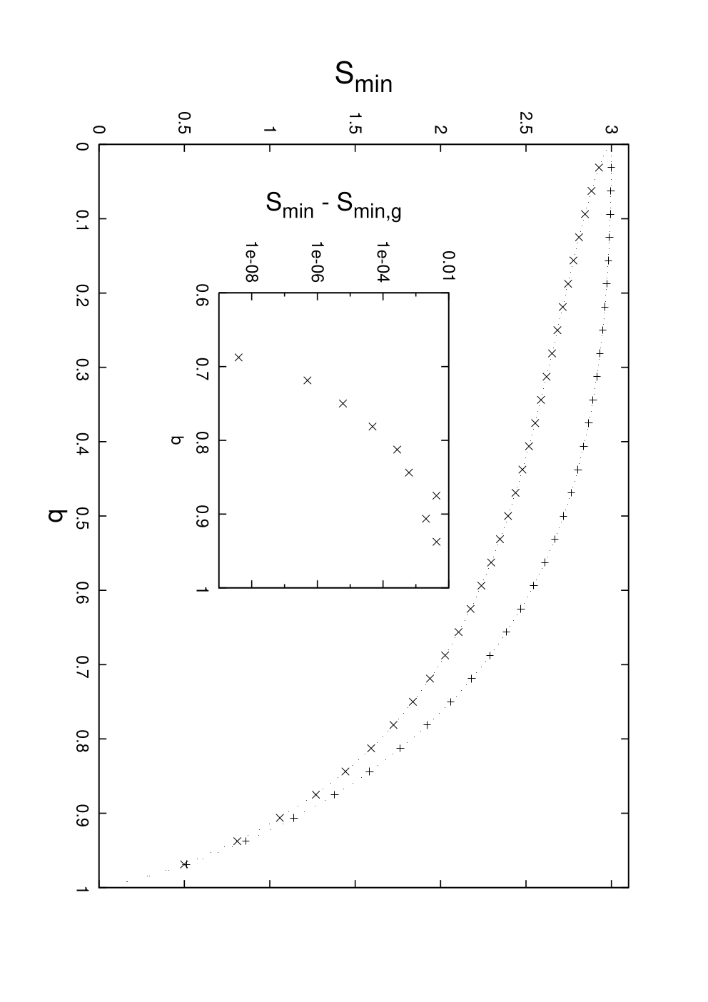
It turns out that the algorithm always converges to the same value of for the symmetric channel . A typical deviation for this channel is about which has the same order of magnitude as the numerical noise.
As for the non-symmetric channel , the algorithm always converges to the same value of unless is close to . A typical deviation is about in the region , so it is not shown on the plot. The deviation is always positive however. On the other hand, if is close to , the iterations sometimes converge to a local minimum with a value of exceeding by several percents.
Numerical simulations have been also carried out for analogous -qubit channels. A plot on Figure 2 shows the smallest output entropy found by the algorithm for a symmetric channel defined as
| (47) |
and for a channel with a non-trivial distribution of the coefficients , namely
| (48) |
Here is a parameter specifying the channel.
The algorithm always converges to the same value of for the symmetric channel . A typical deviation for this channel is about .
For the channel the algorithm always converges to the same value of in a region . The deviation drops down to in a region , so it is not shown on the plot.
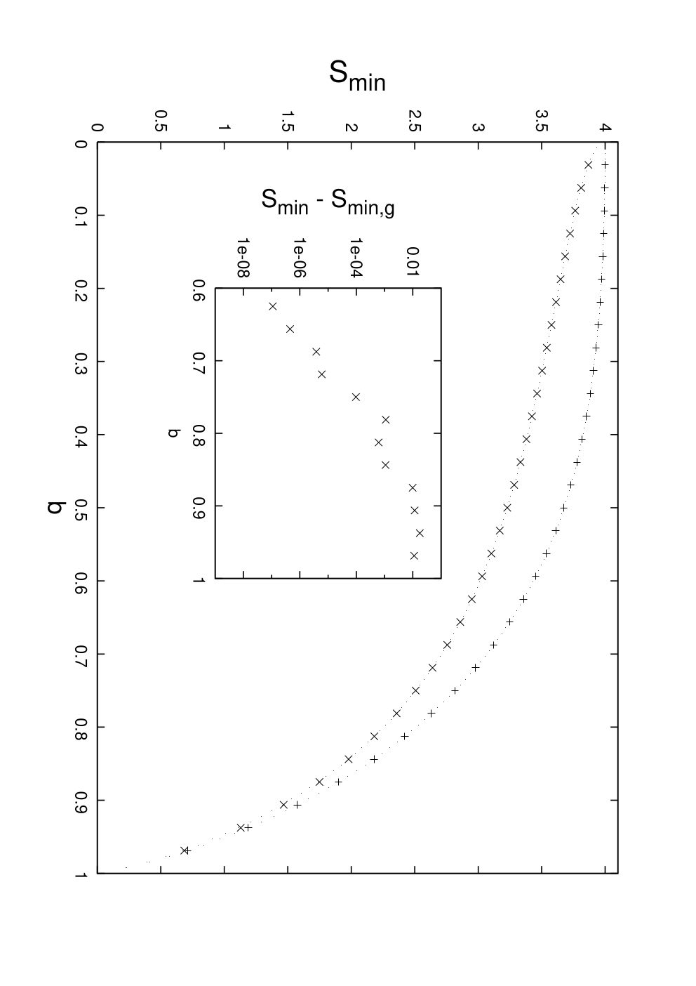
The numerical results seem to support the conjecture that the minimum output entropy is achieved on a Gaussian input state, i.e., that for all fermionic product channels. The fact that the algorithm always converges to the same value of for the symmetric channels suggests that a landscape of the corresponding objective function is particularly simple. It might be an indication that can be computed analytically for the symmetric channels.
VI Acknowledgments
Discussions with Christopher King and Frank Verstraete are gratefully acknowledged. This work was supported by the National Science Foundation under grant number EIA-0086038.
References
- (1) B. Schumacher and M. Westmoreland, Phys. Rev. A 56, no. 1, p. 131 (1997).
- (2) A. S. Holevo, IEEE Transactions on Information Theory 44(1), p. 269 (1998).
- (3) C. King, J. Math. Phys. 43, no 10, p. 4621 (2002).
- (4)
V. Giovannetti,
S. Guha,
S. Lloyd,
L. Maccone,
J.H. Shapiro, and H.P. Yuen, Phys. Rev. Lett. 92, 027902 (2004). - (5) A.S. Holevo and R.F. Werner, Phys. Rev. A 63, 032312 (2001).
- (6) B. Terhal and D. DiVincenzo, Phys. Rev. A 65, 032325 (2002).
- (7) S. Bravyi, Quantum Inf. and Comp. 5, no. 3, p. 216 (2005).
- (8) A.S. Holevo, quant-ph/0212025.
- (9) J. Cortese, quant-ph/0211093.
- (10) V. Giovannetti, S. Guha, S. Lloyd, L. Maccone, and J.H. Shapiro, Phys. Rev. A 70, 032315 (2004).
- (11) E. Knill, quant-ph/0108033.
- (12) A. Marshall and I. Olkin, “Inequalities: Theory of Majorization and Its Applications”, Academic Press (1979).