Quantification of Complementarity in Multi-Qubit Systems
Abstract
Complementarity was originally introduced as a qualitative concept for the discussion of properties of quantum mechanical objects that are classically incompatible. More recently, complementarity has become a quantitative relation between classically incompatible properties, such as visibility of interference fringes and ”which-way” information, but also between purely quantum mechanical properties, such as measures of entanglement. We discuss different complementarity relations for systems of 2-, 3-, or n qubits. Using nuclear magnetic resonance techniques, we have experimentally verified some of these complementarity relations in a two-qubit system.
pacs
03.65.Ta, 03.65.Ud, 76.60.-kI Introduction
Complementarity is one of the most characteristic properties of quantum mechanics, which distinguishes the quantum world from the classical one. In 1927, BohrBohr first reviewed this subject, observing that the wave- and particle-like behaviors of a quantum mechanical object are mutually exclusive in a single experiment, and referred to this as complementarity. Probably the most popular representation of Bohr complementarity is the ‘wave-particle duality’Feynman; Scully, which is closely related to the long-standing debate over the nature of light Simonyi. This type of complementarity is often illustrated by means of two-way interferometers: A classical particle can take only one path, while a classical wave can pass through both paths and therefore display interference fringes when the two partial waves are recombined. Depending on their state, quantum mechanical systems (quantons) can behave like particles (go along a single path), like waves (show interference), or remain in between these extreme cases by exhibiting particle- as well as wave-like behavior. This can be quantified by the predictability , which specifies the probability that the system will go along a specific path, and the visibility of the interference fringes after recombination of the two partial waves, which quantifies the wavelike behavior. A quantitative expression for the complementarity is the inequality Wootters; Bartell; Greenberger; Mandel; JaegerSV; Englert
| (1) |
which states that the more particle-like a system behaves, the less pronounced the wave-like behavior becomes.
In composite systems, consisting of two (or more) quantons, it is possible to optimize the “which-way” information of one particle: one first performs an ideal projective measurement on the second particle. By an appropriate choice of the measurement observable, one can then maximize the predictability for the first partial system. This optimized property, which is called distinguishability , obeys a similar inequality Wootters; Bartell; Greenberger; Mandel; JaegerSV; Englert:
| (2) |
For pure states, the limiting equality holds,
| (3) |
while the inequality holds for mixed states. This issue has been experimentally investigated in the context of interferometric experiments, using a wide range of physical objects including photonsTaylor, electronsMollenstedt, neutronsZeilinger, atomsCarnal and nuclear spins in a bulk ensemble with nuclear magnetic resonance (NMR) techniques Zhu; Peng.
In systems of strongly correlated pairs of particles, it is often useful to consider particle pairs as composite particles with an independent identity. Such composite particles that consist of identical particles include pairs of electrons (Cooper pairs) and photon pairsGhosh. Many interesting phenomena, such as superconductivity, are much easier to understand in terms of the composite particles than in terms of the individual particles. Suitable experiments, such as two-photon interference Ghosh; All can measure properties of the composite particles. These experiments made it possible to quantify the “compositeness” of a two-particle state. Extreme cases are product states, which show no signal in two-particle interference experiments, while maximally entangled states maximize the two-particle visibility but show vanishing visibility in experiments testing the interference of individual particles HorneZeil. Between these extremes lies a continuum of states for which the complementarity relation
| (4) |
holds, which is valid for bipartite pure statesJaegerSV; JaegerHS. Here, is the single-particle visibility for particle , while represents the two-particle visibility. This intermediate regime of the complementarity relation of one- and two-photon interference has only recently been experimentally demonstrated in a Young’s double-slit experiment by Abouraddy et al.Abouraddy.
From a quantum information theoretic point of view, composite quantum systems involve inevitably the concept of entanglement, which is a uniquely quantum resource with no classical counterpart. Does entanglement constitute a physical feature of quantum systems that can be incorporated into the principle of complementarity? Some authors have explored this question and obtained some important results, such as the complementarities between distinguishability and entanglementOHHHH, between coherence and entanglementSAST and between local and nonlocal informationBH etc. Additionally, some complementarity relations in n-qubit pure systems are also observed such as the relationships between multipartite entanglement and mixedness for special classes of n-qubit systemsJSST, and between the single particle properties and the n bipartite entanglements in an arbitrary pure state of n qubitsTessier.
More recently, Jakob and BergouJB derived a generalized duality relation between bipartite and single partite properties for an arbitrary pure state of two qubits, which in some sense accounts for many previous results. They showed that an arbitrary normalized pure state of a two-qubit system satisfies the expressionJB :
| (5) |
Here the concurrence Wootters1998; Wootters2001 is defined by
| (6) |
as a measure of entanglement. is the y component of the Pauli operator on qubit and is the complex conjugate of . The concurrence is a bipartite quantity, which quantifies quantum nonlocal correlations of the system and is taken as a measure of the bipartite character of the composite system. The complement
| (7) |
combines the single-particle fringe visibility and the predictability . This quantity is invariant under local unitary transformations (though and are not), and is therefore taken as a quantitative measure of the single-particle character of qubit .
Since the two-particle visibility is equal to the concurrence, JB, we can rewrite Eq. (5) as
| (8) |
This turns the inequality (4) into an equality and identifies the missing quantity as the predictability .
For pure bipartite systems, an equation similar to Eq. (3) holds, . Here, the index refers to the different particles as the interfering objects in the bipartite system. Combining this with Eq. (5), we obtain
| (9) |
Apparently, contains both the a priori WW information and the additional information encoded in the quantum correlation to an additional quantum system which serves as the possible information storage. This quantum correlation can be measured by the concurrence. This reveals explicitly that quantum correlation can help to optimize the information that can be obtained from a suitable measurement; without entanglement, the available WW information is limited to the a priori WW knowledge .
For mixed states, a weaker statement for the complementarity (5) is found in the form of an inequality . However, there is no corresponding inequality for the two-particle visibility in the mixed two-particle sources because it is very difficult to get a clear and definite expression for and the direct relation between concurrence and two-particle visibility ceases to exist for mixed statesJB.
In this paper, we give a proof-of-principle experimental demonstration of the complementarities (3), (5) and (8) in a two-qubit system. In addition, we extend the complementarity relation (5) to multi-qubit systems. The remainder of the paper is organized as follows: In Sec II, we introduce NMR interferometry as a tool for measuring visibilities and which-way information. Sec. III and Sec. IV discuss measurements of the visibilities and the ”which-way” information in pure bipartite systems. Sec. V is an experimental investigation of the complementarity relation for a pure bipartite system on the basis of liquid-state NMR. For this purpose, we express the entanglement (concurrence) in terms of directly measurable quantities: the two-particle visibility and the distinguishability . This allows us to test two interferometric complementarities (8) and (3) by specific numerical examples. In section VI we generalize the complementarity relation (5) to multi-qubit systems. A quantitative complementarity relation exists between the single-particle property and the bipartite entanglement between the particle and the remainder of the system in pure multi-qubit systems. This allows us to derive, for pure three-qubit system, a relation between the single-particle, bipartite and tripartite properties, which should generalize to arbitrary pure states of qubit systems. Finally, a brief summary with a discussion is given in Sec. VII.
II NMR interferometry
Complementarity relations are often discussed in terms of photons or other particles propagating along different paths. Another, very flexible approach is to simulate these systems in a quantum computer. In particular liquid-state NMR has proved very successful for such investigations. Optical interferometers can readily be simulated by NMR-interferometry Su88.

Figure 1 shows how such an interferometric experiment can be implemented by a sequence of radio-frequency pulses. Assuming an ideal spin particle, the Hilbert space associated with the particle is spanned by vectors and . A beam splitter, which puts the particle incoming from one port into a superposition of both paths is realized by a radio frequency pulse that puts the spin in a superposition of the two basis states. If the flip angle of the pulse is taken as , it corresponds to a symmetric beam splitter. A relative phase shift between the two paths, which corresponds to a path length difference, can be realized by a rotation of the spin around the z-axis. The second radio frequency pulse recombines the two paths.
For the discussion of the complementarity of interference vs. “which-way” information, we consider the superposition state behind the first beam splitter as the starting point. The action of the phase shifter and the second beam splitter can then be summarized into a transducer. Mathematically, this transducer maps the input state into an output state by the transformation
| (10) |
In the NMR interferometer, a number of different possibilities exist for implementing the action of the transducer. We chose the following pulse sequence, which provides high fidelity for a large range of experimental parameters:
| (11) |
Here, we have used the usual convention that refers to an rf pulse with flip-angle and phase .
The resulting populations of both states in the output space vary with the phase angle . As shown in Fig. 1, they can be read out by first deleting coherence with a field gradient pulse (FGP) and then converting the population difference into observable transverse magnetization by a read-out pulse. The amplitude of the resulting FID (= the integral of the spectrum) measures then the populations:
where we have taken into account that the sum of the populations is unity. The experimental signal can be normalized to the signal of the system in thermal equilibrium.
Figure 2 shows, as an example, the interference pattern for the single proton spin in H2O. The amplitude of the spectral line shows a sinusoidal variation with the phase angle , which implies the sinusoidal variation of the population or .
The visibility of the resulting interference pattern is defined as
| (12) |
where or , and and are the minimal and maximal populations (as a function of ).

Since an input state
| (13) |
with an initial Bloch vector and Pauli spin operators is transformed into
| (14) |
with by the transducer, we find for the visibility
| (15) |
and for the predictability
| (16) |
With the described experiment, it is thus straightforward to verify the inequality (1).
III Visibilities in bipartite systems
III.1 Theory
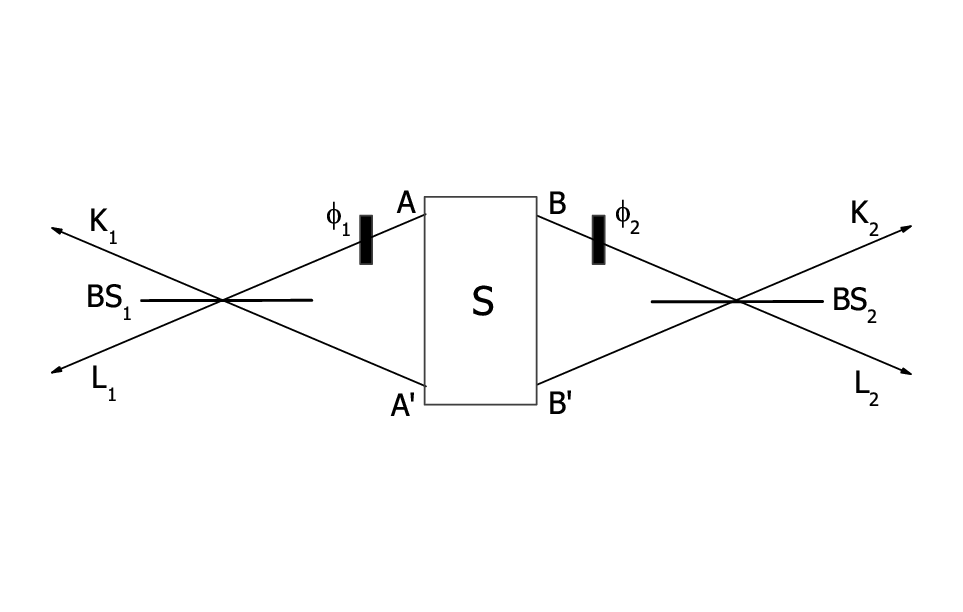
The NMR interferometry experiment can easily be expanded to multi-qubit systems. We start with a discussion of pure bipartite systems, where we explore the visibility in different types of interferometric experiments, geared towards single- and bipartite properties. Figure 3 shows the reference setup: The source S emits a pair of particles 1 and 2, one of which propagates along path and/or , through a variable phase shifter impinging on an ideal beam splitter BS1, and is then registered in either beam or . On the other side there is the analogous process for the other particle with paths and .
Without loss the generality, we first associate states and in Fig. 3 with the spin-up state and , , , and with the spin-down state . A particle pair emitted from the source S can be expressed as the general pure two-qubit state :
| (17) |
with complex coefficients that are normalized to 1.
Assuming that the transducers consist of variable phase shifters and symmetric beam splitters, they can be described by the unitary operation
| (18) |
where each transducer is defined according to Eq. (10). Here the subscripts label two different particles. Applying the transducer (18) to the initial state (17), we can calculate the detection probabilities in the output channels as
| (19) |
where or , and . The single particle count rates reach their maxima and minima when the phase shifters are set to . From Eqs. (12) and (19), the single particle visibilities can be obtained as
| (20) |
Two-particle properties can be measured by higher order correlations. Following reference JaegerSV; JaegerHS, we use the “corrected” two-particle fringe visibility
| (21) |
where or . The “corrected” joint probability are defined such that single-particle contributions are eliminated JaegerSV; JaegerHS. denotes the probabilities of joint detections. As the visibilities explicitly depend on the form of the transducers involved and the details of the measurement (e.g., the measurement basis , is chosen as , ), we use the symbols , here, to indicate the experimental visibilities under a specific experimental configuration, as opposed to the maximal visibilities , .
The “corrected” two-particle joint probabilities can be calculated as
| (22) |
where
| (23) |
The maximal and minimal values of are thus
| (24) |
These values are reached only when the phase shifters are set to , where the parameters can be . Hence, on substituting for the maximal and minimal values of these probabilities in Eq. (21), we find
| (25) |
With Eqs. (20), (23), and (25), the complementarity relation (4) is obtained, valid for arbitrary pure bipartite states.
III.2 Experiments on two extreme cases
For the experimental measurements, we used the nuclear spins of 13C-labeled chloroform as a representative 2-qubit quantum system. We identified the spin of the 1H nuclei with particle 1 and the carbon nuclei (13C) with particle 2. The spin-spin coupling constant between 13C and 1H is 214.95 Hz. The relaxation times were measured to be and for the proton, and and for the carbon nuclei. Experiments were performed on an Infinity+ NMR spectrometer equipped with a Doty probe at the frequencies 150.13MHz for 13C and at 599.77MHz for 1H, using conventional liquid-state NMR techniques.
For most of the experiments that we discuss in the following, the system was first prepared into a pseudo-pure state . Here, is the unity operator and a small constant of the order of determined by the thermal equilibrium. We used the spatial averaging technique PPS and applied the pulse sequence:
| (26) |
where is a field gradient pulse that destroys the transverse magnetizations. The upper indices of the pulses indicate to which qubit the rotation is applied.
Starting from this pseudo-pure state, we then prepared the two-particle source states . As an example, we consider a product state
| (27) |
and a maximally entangled state
| (28) |
They can be prepared from by the following pulse sequences :
| (29) |
where represents a free evolution for this time under the scalar coupling.
The actual interferometer was realized by applying the transducers of Eq. (18) to the prepared state , which describes the effect of the phase shifters and symmetric beam splitters. The transducer pulse sequence (11) is simultaneously applied to both qubits.
The probabilities that enter the complementarity relations can be expressed in terms of populations of the four spin states. To determine these spin states, we used a simplified quantum state tomography scheme to reconstruct only the diagonal elements of the density matrix. This was realized by
| (30) |
for . represents to recording the FID of qubit after a field gradient pulse and a read-out pulse . Fig. 4 shows the NMR signals after Fourier transformation of the corresponding FIDs for the proton and carbon spins in 13CHCl3 at when they are prepared in the product state or the maximally entangled state .

The signals measure the populations:
| (31) |
where for the high-frequency resonance line and for the low-frequency line.
To create an interferogram, we varied the phases from to , incrementing both simultaneously in steps of . The resulting interference pattern of the proton is shown in Fig. 5.

The carbon signals have a similar behavior as a function of for the states and , as Fig. 5 shows. From these experimental data points, we calculated the probabilities and and fitted those to a cosine function: . From the fitted values of the amplitude and the offset , we extracted the experimental visibilities as , for the product state and , for the entangled state by the definitions of Eqs.(12) and (21). As theoretically expected, the product state shows one-particle interference fringes, but almost no two-particle interference fringes, while the situation is reversed for the entangled state . It can also be seen that the discrepancies from the theory is larger for the entangled state than for the product state . This is easily understood by realizing that the state preparation is more complicated for the entangled state.
IV ”Which-way” information in bipartite systems
IV.1 Predictability
For the same system, we can calculate the predictabilities, i.e. the probabilities for correctly predicting which path the particle will take, from the expectation value of the observable on the state , i.e., :
| (32) |
where is the z component of the Pauli operator on qubit . is thus the magnitude of the difference between the probabilities that particle takes path or the other path .
For the experimental measurement of the predictability , we measure the observable by partial quantum state tomography: a field gradient pulse destroys coherences and a readout pulse converts into , which is recorded as the FID. Upon Fourier transformation, the integral of both lines yields , and its magnitude corresponds to the predictability .
Figure 6 shows the measurement of the predictability on 13CHCl3 for two specific examples: the product state and the entangled state .

IV.2 Distinguishability
In a bipartite system, the which-way information for particle can be optimized by first performing a projective measurement on particle . For this measurement, we first have to choose the optimal ancilla observable . According to Englert’s quantitative analysis of the distinguishabilityEnglert, we start by writing the quantum state as the sum of two components corresponding to two paths of qubit :
| (33) |
Each component is coupled to a different state of qubit :
| (34) |
The coefficients are
| (35) |
A suitable measurement is performed on qubit to make qubit acquire the maximal “which-way” information. To determine the most useful ancilla observable, we write it as . The probability that the ancilla observable finds eigenvalue differs for the two component states:
| (36) |
where is the corresponding eigenvector.
The distinguishability for qubit is obtained by maximizing the difference of the measurement probabilities for the two components,
| (37) |
Using the notation
| (38) |
where are vectors on the Bloch sphere, we write
| (39) |
Clearly the maximum is reached if the two vectors and are parallel. Since has unit length, the distinguishability becomes
| (40) | |||||
Combining Eqs. (20) and (40), we obtain the complementarity relation (3), i.e., for .
For the experimental measurement, we first have to perform a ”measurement” on the ancilla qubit , using the optimal observable . This is done by applying a unitary transformation to rotate the eigenbasis of the observable into the computational basis Brassard. The subsequent field gradient pulse destroys coherence of qubit Teklemariam, as well as qubit and joint coherences (=zero and double quantum coherences). After this ancilla measurement, the distinguishability can be measured by a readout pulse, detection of the FID, Fourier transformation, and taking the sum of the magnitudes of both resonance lines.
Figure 7 shows the observed distinguishability for the states and . From Eq. (39), we find the optimal observable is for , and with for . Therefore, the transformation was realized by the NMR pulses and . As there is no entanglement in the state , , while for the entangled state we find . The experimental data also satisfy the relation of Eq. (9).

V Complementarity relations for bipartite systems
With the same experimental scheme we now explore the complementarity relations for bipartite quantum systems. Between the single particle visibility (see Eq. (20)), the two-particle visibility (Eq. (25)), and the predictability (Eq. (32)), we can verify that the relation
| (41) |
holds in a pure bipartite system for any experimental setting and measurement basis.
If the initial state has only real coefficients , the inequality becomes an equality. In this case, the two-particle visibility becomes equal to the concurrence , . However, when the coefficients are arbitrary complex numbers, the two-particle visibility can be smaller than the concurrence, . As a specific example consider . Using symmetric beam splitters and the measurement basis ), we find and , i.e. .
By the Schmidt decompositionNielsbook, any pure state can be transformed into one with real coefficients by local unitary operations. Therefore, one can design a different experiment using beam splitters that implement the transformation instead of the symmetric one . In this case, the single-particle transducers implement the operation
| (42) |
instead of in Eq. (10). Note that the single-particle character (Eq. (7)) is invariant under local unitary transformations though its constituents and are not. By defining the maximal visibility , we obtain and
| (43) |
This shows that the complementarity relation (8) in the equality form is fulfilled for any pure bipartite system. An alternative way is to keep the symmetric beam splitters and change the measurement basis. One can always choose an optimal basis which consists of the eigenvectors of an observable that maximizes the visibility , i.e., . Being invariant under local unitary transformations, this maximal two-particle visibility (= concurrence ) is a good measure of the bipartite property encoded in the pure state.
In a pure bipartite system, the complementarity relation (43), together with the identity and the definition (7) of the single particle character offers a method for quantifying entanglement in terms of the directly measurable quantities, in this case visibilities, predictability and distinguishability. In this section, we experimentally explore these complementarity relations for the states
| (44) | |||||
by preparing the state in the nuclear spins of molecules, and measuring the visibilities, predictability and distinguishability by NMR according to the procedure outlined above.
| Particle | |||||||||
|---|---|---|---|---|---|---|---|---|---|
|
|
|
Table 1 lists the theoretical expectations for the various quantities involved in the complementarity relation for this state. The single particle character and the concurrence ( the maximal two-particle visibility ) satisfy the duality relation of Eq. (43). For the state (Eq. (44)), the maximal two-particle visibility is obtained from the experimental visibility by setting the measurement basis to the computational basis . The predictabilities for the two particles are qualitatively different, , which results in whereas . The special case with was discussed in detail in Ref.JaegerHS; in that case, both predictabilities vanish, . However, and are still satisfied for or .
To verify these relations, we used an experimental procedure similar to that discussed in Section IIIB. To prepare the state from the pseudo-pure state , we used the following NMR pulse sequence:
| (45) |
When is negative, we generate the required evolution by inserting two pulses on one of the two qubits before and after the evolution period of .
We measured the visibilities for the state by first scanning while fixing to , then repeated the experiment with fixed and variable . This provides the maximal probabilities of the “corrected” joint probabilities, which occur at for .
As a specific example, we present the experimental results for with . The resulting interference fringes were closely similar to those shown in Fig. 5. Using the procedure described in Section IIIB, we extracted the relevant visibilities and from the experimental data. The visibilities and the predictability were measured as a function of varying from to in steps of . The single-particle character and the two-particle visibility from these experiments are displayed in Fig. 8, together with plots of the theoretical complementarity relations (solid curves) indicating for the pure two-qubit states. A fit of these data to the equation resulted in an amplitude for the data of Fig. 8 (a) and for the data of Fig. 8(b).

For the quantitative measurement of the distinguishability , the optimal observable for is a spin operator parallel to with for , in agreement with Ref. Peng, and for , according to the analysis of section IV B. The transformation was realized by a pulse. Figure 9 compares the measured values of the single particle visibilities and the distinguishabilities to the theoretical complementarity relations (solid curves) . The fitted values of the amplitude are for the data in Fig. 9(a) and for Fig. 9(b).

In Fig. 10, we compare two independent ways for measuring the concurrence , either through the two-particle visibility , or through the single-particle quantities, as . Both data sets are plotted against , together with the theoretical concurrence . The figure shows clearly that the two procedure give the same results, within experimental errors. Apparently, both methods allow one to experimentally determine the entanglement of pure two-qubit states. At the same time, the data verify the complementarity relation (5).

In these experiments, the maximal absolute errors for the quantities , and were about . The error is primarily due to the inhomogeneity of the radio frequency field and the static magnetic field, imperfect calibration of radio frequency pulses, and signal decay during the experiments. A maximal experimental error about results for the verification of the complementarity relations. If we take into account these imperfections, the measured data in our NMR experiments agree well with the theory.
VI Multi-qubit systems
To generalize the complementarity relation (5) to multi-qubit systems, we consider a pure state with n qubits . According to the generalized concurrence for pairs of quantum systems of arbitrary dimension by Rungta et al. RBCHM01; RC2003, we calculate the bipartite concurrence between qubit and the system with the remaining qubits in terms of the marginal density operator
| (46) |
In terms of the single particle character (Eq. (7)), and using , we obtain the complementarity relation
| (47) |
This is a first generalization of the tradeoff between individual particle properties, quantified by , and the bipartite entanglement to many particle systems. It implies also the relation derived by TessierTessier.
To characterize the pairwise entanglements of qubit with the other qubits, we sum over the squares of the concurrences of all two-partite subsystems involving qubit ,
| (48) |
Here, the concurrence is defined in terms of the marginal density operator for the subsystem, using the definition of , where are the square roots of the eigenvalues of in decreasing orderWootters1998; Wootters2001.
We now specialize to pure three-qubit systems. Here, it is possible to specify three-partite entanglement by the 3-tangle CKW2000 as
| (49) |
Combining Eqs (47), (48), and (49), we find a complementarity between single-particle properties , pair-wise entanglement , and three-partite entanglement , which is valid for each individual qubit:
| (50) |
For specific examples, we have listed in Table 2 different three-qubit states and calculated the 1-, 2-, and 3-qubit quantifiers appearing in Eq. (50). As can be verified from the table, these states satisfy Eq. (50) in different ways. The product states of the first entry only have single particle character. As discussed by Dür et al. DVC2000, the states listed in the second entry represent bipartite entanglement between the second and third qubit, while the first qubit is in a product state with them. The GHZ states are pure three-particle entangled states, while the W states exhibit no genuine three-particle entanglement, but two- and one particle properties.
| Class | |||
|---|---|---|---|
| 0 | 0 | 1 | |
| 0 | |||
| 0 | |||
| 0 |
Since there is no generalization of the 3-tangle to larger systems, we can only speculate here if it is possible to extend the relation (50) to more than three qubits. On a heuristic basis, we consider two types of pure n-qubit systems. One is a generalization of the GHZ states to n qubits: . This is a state with pure n-way entanglement, i.e.,
| (51) |
where denotes the pure m-tangle regarding qubit . Here, the m-tangle denotes m-way or m-party entanglement that critically involves all m parties, which is different from the I-tangle in Ref. RBCHM01; RC2003 and a recently introduced measure of multi-partite entanglement defined by with a spin-flip operation by A. Wong and N. Christensen WC2001. Currently, there is no general way to measure this form of entanglement beyond three qubits.
The W states of Table 2 may also be generalized to n qubits as . These states exhibit the maximal bipartite entanglements and no other m-way entanglements, i.e.,
| (52) |
In these two cases the complementarity relation generalizes to .
VII Conclusions
Complementarity is a universal relationship between properties of quantum objects. However, it behaves in different ways for different quantum objects. The purpose of this paper was to analyze the different complementarity relations that exist in two- and multi-qubit systems and to illustrate some of them in a simple NMR system.
We experimentally verified the complementarity relation between the single-particle and bipartite properties: in a pure two-qubit system. To determine the entanglement, we used either the two-particle visibility or the distinguishability and the predictability . Accordingly, two complementarity relations: and were tested for different states including maximally entangled, separable, as well as partially entangled (intermediate) states.
Furthermore, the complementarity between one- and two-particle character was generalized to systems of n qubits. The complementarity relation holds for an arbitrary pure n-qubit state, which implies a tradeoff between the local single-particle property () and the nonlocal bipartite entanglement between the particle and the remainder of the system (). More interesting, in a pure three-qubit system, the single-particle character (), the two-particle property regarding this particle measured by the sum of all pair-wise entanglements involving the particle (), and the three-particle property measured by the genuine tripartite entanglement () are complementary, i.e., . However, the generalization of the similar relationship to a larger-qubit system requires the identification and quantification of multi-partite entanglement for pure and mixed states beyond three-qubit systems that still remains an open question currently. A similar relationship cannot be directly generalized to larger qubit systems. Some specific samples might be helpful to conjecture the relation : the single-particle property (local) of a particle might be complementary to all possible pure multi-particle properties (nonlocal) connected to this particle.
Complementarity and entanglement are two important phenomena that characterize quantum mechanics. From these observations, we conclude that entanglement in its various forms is an important parameter for the different forms of complementarity relations in multi-partite systems. Different forms of entanglement quantify the amount of information encoded in the different quantum correlations of the system, indicating the multi-partite quantum attributes. These results have also implications on the connection between entanglement sharing and complementarity and maybe in turn provide a possible way to study the entanglement in multi-partite quantum systems by complementarity. We hope that these findings will be useful for future research into the nature of complementarity and entanglement.
ACKNOWLEDGMENTS
We thank Reiner Küchler for help with the experiments. X. Peng acknowledges support by the Alexander von Humboldt Foundation. This work is supported by the National Natural Science Foundation of China (Grant NO. 10274093 and 10425524) and by the National Fundamental Research Program (2001CB309300).
References
- (1) N. Bohr, 1928 Naturwissenschaften 16 245; Nature (London) 121 580 (1928).
- (2) R. P. Feynman, R. B. Leifhton, and M. Sands, the Feynamn Lectures of Physics, Vol. III. Quantum Mechanics, Addison -Wesley, Reading (1965).
- (3) M. O. Scully, B. -G. Englert and H. Walther, 1991 Nature 351 111.
- (4) K. Simonyi, ”Kulturgeschichte der Physik” Verlag Harri Deutsch, Thun, (1990).
- (5) W. K. Wootters and W. H. Zurek, Phys. Rev. D 19 473 (1979); L. S. Bartell, ibid. 21 1698 (1980); D. M. Greenberger and A. Yasin, Phys. Lett. A 128 391 (1988); L. Mandel, Opt. Lett. 16 1882 (1991).
- (6) L. S. Bartell, Phys. Rev. D 21 1698 (1980).
- (7) D. M. Greenberger and A. Yasin, Phys. Lett. A 128 391 (1988).
- (8) L. Mandel, Opt. Lett. 16 1882 (1991).
- (9) G. Jaeger, A. Shimony and L. Vaidman, Phys. Rev. A 51 54 (1995).
- (10) B. -G. Englert, Phys. Rev. Lett. 77, 2154 (1996); B. -G. Englert, and J. A. Bergou, Opt. Comm. 179, 337 (2000).
- (11) G. I. Taylor, Proc. Camb. Phil. Soc. 15, 114 (1909); P. Mittelstaedt, A. Prieur and R. Schieder, Found. Phys. 17, 891 (1987); P. D. D. Schwindt, P. G. Kwiat and B. -G. Englert, Phys. Rev. A 60, 4285 (1999).
- (12) G. Mllenstedt and C. Jnsson, Z. Phys. 155, 472 (1959); A. Tonomura, J. Endo, T. Matsuda, and T. Kawasaki, Am. J. Phys. 57, 117 (1989).
- (13) A. Zeilinger, R. Ghler, C. G. Shull, W. Treimer, and W. Mampe, Rev. Mod. Phys. 60, 1067 (1988); H. Rauch and J. Summhammer, Phys. Lett. A 104, 44 (1984); J. Summhammer, H. Rauch and D. Tuppinger, Phys. Rev. A 36, 4447 (1987).
- (14) O. Carnal and J. Mlynek, Phys. Rev. Lett. 66, 2689 (1991); S. Drr, T. Nonn and G. Rempe, Phys. Rev. Lett. 81, 5705 (1998); P. Bertet, S. Osnaghl, A. Rauschenbeutel, G. Nogues, A. Auffeves, M. Brune, J. M. Ralmond and S. Haroche, Nature 411, 166 (2001).
- (15) X. Zhu, X. Fang, X. Peng, M. Feng, K. Gao and F. Du, J. Phys. B 34, 4349 (2001).
- (16) X. Peng, X. Zhu, X. Fang, M. Feng, M. Liu, and K. Gao, J. Phys. A 36, 2555 (2003).
- (17) R. Ghosh and L. Mandel, Phys. Rev. Lett. 59, 1903 (1987).
- (18) C. O. Alley and Y. H. Shih, in Proceedings of the Second International Symposium on Foundations of Quantum Mechanics in Light of New Technology, edited by M. Namiki et al. (Physical Society of Japan, Tokyo, 1986), p. 47; Y. H. Shih and C. O. Alley, Phys. Rev. Lett. 61, 2921 (1988); C. K. Hong, Z. Y. Ou, and L. Mandel, Phys. Rev. Lett. 59, 2044 (1987); J. G. Rarity and P. R. Tapster, ibid. 64, 2495 (1990); P. G. Kwiat, W. A. Vereka, C. K. Hong, H. Nathel, and R. Y. Chiao, Phys. Rev. A 41, R2910 (1990); M. Horne, A. Shimony, and A. Zeilinger, in Quantum Coherence, edited by J. Anandan (World Scientific, Singapore, 1990), p. 356.
- (19) M. A. Horne and A. Zeilinger in Proceedings of the Symposium on the Foundations of Modern Physics, edited by P. Lahti and P. Mittelstaedt (World Scientific, Singapore, 1985), p435.
- (20) G. Jaeger, M. A. Horne and A. Shimony, Phys. Rev. A 48, 1023 (1993).
- (21) A. F. Abouraddy, M. B. Nasr, B. E. A. Saleh, A. V. Sergienko and M. C. Teich, Phys. Rev. A 63, 063803 (2001).
- (22) J. Oppenheim, K. Horodecki, M. Horodecki, P. Horodecki, and R. Horodecki, Phys. Rev. A 68, 022307 (2003)
- (23) B. E. A. Saleh, A. F. Abouraddy, A. V. Sergienko, and M. C. Teich, Phys. Rev. A 62, 043816 (2000).
- (24) S. Bose and D. Home, Phys. Rev. Lett. 88, 050401 (2002).
- (25) G. Jaeger, A. V. Sergienko, B. E. A. Saleh, and M. C. Teich, Phys. Rev. A 68, 022318 (2003).
- (26) T. E. Tessier, Found. Phys. Lett. 18, 107 (2005), also see arXiv: quant-ph/0302075.
- (27) M. Jakob and J. A. Bergou, arXiv: quant-ph/0302075.
- (28) W. K. Wootters, Phys. Rev. Lett. 80, 2245 (1998).
- (29) W. K. Wootters, Quantum. Inf. Comput. 1, 27 (2001).
- (30) D. Suter, K. T. Mueller, and A. Pines, Phys. Rev. Lett., 60, 1218 (1988).
- (31) D. G. Cory, A. F. Fahmy and T. F. Havel, Proc. Natl. Acad, Sci. USA, 94, 1634 (1997); N. A. Gershenfeld and I. L. Chuang, Science, 275, 350 (1997) .
- (32) G. Brassard, S. Braunstein and R. Cleve, Phys. D 120, 43 (1998).
- (33) G. Teklemariam, E. M. Fortunato, M. A. Pravia, T. F. Havel, and D. G. Cory, Phys. Rev. Lett. 86, 5845 (2001).
- (34) M. A. Nielsen and I. L. Chuang, Quantum Computation and Quantum Information (Cambridge Univ. Press, Cambridge, 2000).
- (35) P. Rungta and C. M. Caves, Phys. Rev. A 67, 012307 (2003).
- (36) P. Rungta, V. Buzek, C.M. Caves, M. Hillery, and G.J. Milburn, Phys. Rev. A 64, 042315 (2001).
- (37) V. Coffman, J. Kundu and W. K. Wootters, Phys. Rev. A 61, 052306 (2000).
- (38) W. Dr, G. Vidal and J. I. Cirac, Phys. Rev. A 62, 062314 (2000).
- (39) A. Wong and N. Christensen, Phys. Rev. A 63, 044301 (2001).