Dense coding with multipartite quantum states

Entanglement among quantum systems can be used to perform tasks that are not possible with classical states. Phenomena where entanglement plays a crucial role include e.g. teleportation [1] and dense coding [2]. In the dense coding protocol, entangled quantum states are used to send classical information from a sender (say, Alice) to a receiver (say, Bob). Suppose that Alice wants to send two bits of classical information to Bob. Then the Holevo bound, to be discussed later, shows that Alice must send two qubits (two-dimensional quantum states) to Bob, if only a noiseless quantum channel is available. However, if Alice and Bob have previously shared entanglement, then Alice may have to send less than two qubits to Bob. It was shown by Bennett and Wiesner [2], that by using a previously shared singlet, Alice will be able to send two bits to Bob, by transmitting just a single qubit.

To consider a realistic scenario, two avenues are usually taken. One approach is to consider a noisy quantum channel, where the additional resource is an arbitrary amount of shared bipartite pure state entanglement (see e.g. [3, 4, 5, 6]). This is the scenario of the so-called entanglement assisted capacity, which refers to a property of the channel. The other approach is to consider a noiseless quantum channel, while the assistance is by a given bipartite mixed entangled state (see e.g. [5, 6, 7, 8, 9, 10]). In this second case the capacity refers to a feature of the state. In this paper, we consider the second approach, in the general situation of several senders and one or two receivers. Therefore the senders and the receiver(s) share a given multiparty state. The senders (called Alices, and named as $A_{1},A_{2},\cdots,A_{N}$) want to send classical information to the receivers (Bobs, $B_{1}$ and $B_{2}$), where the information of one Alice can be different from that of another. All the parties that take part in the protocol are at distant locations. Consequently, both the encoding of the information by the Alices, and the decoding of it by the Bobs, must be by local operations. Additionally, the Alices can communicate between themselves over a classical channel, and likewise the Bobs can do so between themselves. Classical communication is of course not allowed between the senders and the receivers.

We considered this scenario in Ref. [11], and named it “distributed quantum dense coding”. In this paper, we further discuss the bounds on the capacity of dense coding in this scenario, for a given state, where the capacity is defined as the number of classical bits that can be accessed by the receivers, per use of the noiseless channel. Also, we give a classification of multipartite states according to their degree of ability to assist in distributed dense coding.

The paper is organized as follows. In Section 2 we discuss the Holevo bound, which is a crucial element in finding the capacity of dense coding for the case of a single receiver. In Section 3, we consider the case of dense coding with a single sender and a single receiver. In Section 4, we take up the case of many senders but a single receiver, and find the capacity in this scenario. We show that the capacity is not enhanced by allowing the senders to perform joint operations. To consider the case of many receivers, we must obtain a Holevo-like upper bound on classical information that can be decoded from multiparty quantum ensembles. Such a bound, derived in Ref. [13] for bipartite ensembles, is discussed in Section 5. In Sec. 6 we obtain an upper bound of dense coding schemes for an arbitrary number of senders and two receivers (a bound for multiparty ensembles is currently absent [14]). In Sec. 7, we will discuss a classification of multiparty states according to their degree of usefulness in dense coding protocols and give some examples. In Sec. 8 we will summarize our results and discuss some related open problems.

The Holevo bound is an upper bound on the amount of classical information that can be accessed from a quantum ensemble in which the information is encoded. Suppose that Alice ($A$) has the classical message $i$ that occurs with probability $p_{i}$. Alice encodes this information $i$ in a quantum state $\rho_{i}$, and sends it to Bob. Bob receives the ensemble $\{p_{i},\rho_{i}\}$, and wants to obtain as much information as possible about $i$. To do so, he performs a measurement, that gives the result $m$ with probability $q_{m}$. Let the corresponding post-measurement ensemble be $\{p_{i|m},\rho_{i|m}\}$. The information gathered can be quantified by the mutual information between the message index $i$ and the measurement outcome [15]:

Here $H(\{r_{x}\})=-\sum_{x}r_{x}\log_{2}r_{x}$ is the Shannon entropy of the probability distribution $\{r_{x}\}$. Bob will be interested to obtain the maximal information, which is maximum of $I(i:m)$ for all measurement strategies. This quantity is called the accessible information:

where the maximization is performed over all measurement strategies.

The maximization involved in the definition of accessible information is usually hard to compute, and hence the importance of bounds [12, 16]. In particular, in Ref. [12], a universal upper bound on $I_{acc}$, the Holevo bound, is given (see also [17, 13, 18])

Here $\overline{\rho}=\sum_{i}p_{i}\rho_{i}$ is the average ensemble state, and $S(\varsigma)=-\mbox{tr}(\varsigma\log_{2}\varsigma)$ is the von Neumann entropy of $\varsigma$. The Holevo bound is asymptotically achievable in the sense that if the sender is able to send long strings of the input quantum states $\rho_{i}$, then there exists a particular encoding and a decoding scheme that asymptotically attains the bound [19].

Suppose that Alice and Bob share a quantum state $\rho^{AB}$. Alice performs the unitary operation $U_{i}$ with probability $p_{i}$, on her part of the state $\rho^{AB}$ to encode the classical information $i$. Subsequent to her unitary rotation, she sends her part of the state $\rho^{AB}$ to Bob. Bob then has the ensemble $\{p_{i},\rho_{i}\}$, where

The information that Bob is able to gather is $I_{acc}(\{p_{i},\rho_{i}\})$. This quantity is bounded from above by $\chi(\{p_{i},\rho_{i}\})$. The “one-capacity” $C^{(1)}$ of dense coding for the state $\rho^{AB}$ is the Holevo bound for the best encoding by Alice:

The superscript $(1)$ reflects the fact that Alice is using the shared state once at a time, during the asymptotic process. She is not using entangled unitaries on more than one copy of her parts of the shared states $\rho^{AB}$. As we will see below, encoding with entangled unitaries does not help her to send more information to Bob.

In performing the maximization in Eq. (5), first note that the second term in the right hand side (rhs) is equal to $-S(\rho)$, for all choices of the unitaries and probabilities, as unitary operations do not change the spectrum, and hence the entropy, of a state. Secondly, we have

where $d_{A}$ is the dimension of Alice’s part of the Hilbert space of $\rho^{AB}$, and $\overline{\rho}^{A}=\mbox{tr}_{B}\overline{\rho}$, $\overline{\rho}^{B}=\mbox{tr}_{A}\overline{\rho}$. Moreover, $S(\overline{\rho}^{B})=S(\rho^{B})$, as nothing was done at Bob’s end during the encoding procedure. Therefore, we have

This bound is reached by any complete set of orthogonal unitary operators $\{W_{j}\}$, to be chosen with equal probabilities, which satisfy the trace rule $\frac{1}{d_{A}}\sum_{j=1}^{d_{A}}W_{j}^{\dagger}\Xi W_{j}=\Tr[\Xi]I$, for any operator $\Xi$. Therefore, we have

The optimization procedure above essentially follows that in Ref. [9]. Several other lines of argument are possible for the maximization. One approach is given in Ref. [8] (see also [11]). Another way to proceed is to guess where the maximum is reached, and then perturb the guessed result. If the first order perturbations vanish, the guessed result is correct, as the von Neumann entropy is a concave function and the maximization is carried out over the continuous set of all $\{p_{i},U_{i}\}$ [11]. Note here that without using the additional resource of entangled states, Alice will be able to reach a capacity of just $\log_{2}d_{A}$ bits. Therefore, entanglement in a state $\rho^{AB}$ is useful for dense coding if $S(\rho^{B})-S(\rho)>0$. Such states exist, an example being the singlet state.

Suppose now that there are $N$ Alices, viz. $A_{1}$, $A_{2}$, $\cdots$, $A_{N}$, who want to send information to a single receiver, Bob ($B$). They share the quantum state $\rho^{A_{1}A_{2}\cdots A_{N}B}$. Depending on the classical information $i_{k}$ that $A_{k}$ wants to send to Bob, she applies the unitary operation $U_{i_{k}}$ with probability $p_{i_{k}}$ ($k=1,2,\cdots,N$). After applying the unitary operations, they send their parts of the quantum state to Bob, who has now the ensemble $\{p_{\{i\}},\rho_{\{i\}}\}$, where $\{i\}$ denotes the string $\{i_{1},i_{2},\cdots,i_{N}\}$. Moreover

where $U_{\{i\}}=U_{i_{1}}\otimes U_{i_{2}}\otimes\cdots\otimes U_{i_{N}}$. The task of Bob is to obtain as much information as possible about the message string $\{i\}$. Since the Holevo bound is asymptotically attainable by product encoding (Section 2), the “one-capacity” of the state $\rho^{A_{1}A_{2}\cdots A_{N}B}$ in this case is defined as

To avoid multiple indices, we use the same notation as in the case of a single sender. As we will see, the capacities in the case of a single sender and multiple senders are the same (at least in the case when there is only a single receiver). Analogous considerations as for the maximization of Eq. (5) lead to

where $d_{A_{k}}$ is the dimension of the Hilbert space in possession of the $k$th Alice $A_{k}$. Moreover by similar arguments as in Section 3.1, also in this case, the one-capacity can be shown to be the asymptotic capacity, so that

Again, we use the same notation as in the case of a single sender. The capacity is reached by any complete set of orthogonal unitaries that satisfies the trace rule. However such a complete orthogonal set of unitaries of the $A_{1}A_{2}\cdots A_{N}$ space can be formed by product unitaries of the individual spaces of the $A_{k}$. This leads us to the conclusion that even if the Alices are allowed to perform entangled unitaries, this will not enhance the dense coding capacity of the state $\rho^{A_{1}A_{2}\cdots A_{N}B}$. We will illustrate the case of many Alices in detail for clarity. However, as long as one considers unitary encodings, it is clear that the Holevo bound is the same for factorised unitaries, and many Alices are equivalent to a single one with the according dimension.

The Holevo bound is an upper bound on the accessible information encoded in a quantum ensemble that is sent to a single receiver. This is also an upper bound on the accessible information encoded in a quantum ensemble that is sent to two receivers, where the receivers are allowed to perform only local operations and classical communication (LOCC). However, in Ref. [13], we have obtained an independent upper bound for this situtation. (For a lower bound, see Ref. [24].) Suppose that a sender encodes the classical message $i$ in the bipartite quantum state $\rho^{B_{1}B_{2}}_{i}$ with probability $p_{i}$, and sends it to two Bobs (Bob1 ($B_{1}$) and Bob2 ($B_{2}$)). The tasks of the Bobs is to gather as much information as posssible about $i$. Let the accessible information in this situation be called “locally accessible information”, denoted by $I_{acc}^{LOCC}$. It was shown in Ref. [13] that

where $\rho_{i}^{B_{1}}=\Tr_{B_{2}}\rho_{i}^{B_{1}B_{2}}$, $\rho_{i}^{B_{2}}=\Tr_{B_{1}}\rho_{i}^{B_{1}B_{2}}$, $\overline{\rho}^{Z}=\sum p_{i}\rho_{i}^{Z}$, $Z=B_{1},B_{2}$.

This bound is not necessarily better than the Holevo bound for all ensembles. For example, for the ensemble formed by the states $|00\rangle$, $|11\rangle$, taken with probability $\frac{1}{2}$ each, the Holevo bound equals $1$, while our local bound $\chi^{LOCC}$ is $2$. This, of course, implies that the bound $\chi^{LOCC}$ on $I_{acc}^{LOCC}$ is asymptotically not attainable in general. However, there are important examples for which the local bound ($\chi^{LOCC}$) is drastically smaller than the global one ($\chi$). For example, for the four Bell states $|\psi^{\pm}\rangle,|\phi^{\pm}\rangle$, chosen with probabilities $p_{i}$ ($i=1,2,3,4$), $\chi=H(\{p_{i}\})$, while $\chi^{LOCC}=1$. In particular, for equal apriori probabilities, the global bound is 2, while the local one is still unity.

We will now consider the case of dense coding with two receivers. Suppose therefore that $N$ Alices ($A_{1},A_{2},\cdots,A_{N}$) and two Bobs ($B_{1}$ and $B_{2}$) share a quantum state $\rho^{A_{1},A_{2},\cdots,A_{N}B_{1}B_{2}}$. To send the classical information $i_{k}$, $A_{k}$ performs the unitary operation $U_{i_{k}}$, with probability $p_{i_{k}}$. Then the Alices send their part of the resulting state to the Bobs. For definiteness, let us assume that $A_{1},A_{2},\cdots,A_{M}$ send their parts of the resulting state to $B_{1}$, while the rest of the Alices send to $B_{2}$. Hence the Bobs receive the ensemble $\{p_{\{i\}},\rho_{\{i\}}\}$, where $p_{\{i\}}=p_{i_{1}}p_{i_{2}}\cdots p_{i_{N}}$, $\rho_{\{i\}}=U_{\{i\}}\otimes\Id\otimes\Id\rho^{A_{1}A_{2}\cdots A_{N}B_{1}B_{2}}U_{\{i\}}^{\dagger}\otimes\Id\otimes\Id$, with $U_{\{i\}}=U_{i_{1}}\otimes U_{i_{2}}\otimes\cdots\otimes U_{i_{N}}$. Let us warn here that the same notation $\rho_{\{i\}}$ was used in the case of a single receiver in Section 4, although the situation there is different than this one. The aim of the Bobs is to gather maximal information from the ensemble $\{p_{\{i\}},\rho_{\{i\}}\}$ about the message string $\{i\}=\{i_{1},i_{2},\cdots,i_{N}\}$, but they are restricted to perform only LOCC between themselves. The “one-capacity” in this case is

so that

where the ensemble states $\rho_{\{i\}}$ in the two above equations is to be considered in the $A_{1}A_{2}\cdots A_{M}B_{1}:A_{M+1}A_{M+2}\cdots A_{N}B_{2}$ bipartite split, for calculating the locally accessible information and its local bound. We have

where $\rho_{\{i\}}^{\textbf{1}}=\Tr_{A_{M+1}\cdots A_{N}B_{2}}\rho_{\{i\}}^{A_{1}\cdots A_{N}B_{1}B_{2}}$, $\rho_{\{i\}}^{\textbf{2}}=\Tr_{A_{1}\cdots A_{M}B_{1}}\rho_{\{i\}}^{A_{1}\cdots A_{N}B_{1}B_{2}}$, and $\overline{\rho}^{\textbf{Z}}=\sum p_{\{i\}}\rho_{\{i\}}^{\textbf{Z}},\textbf{Z}=\textbf{1},\textbf{2}$.

The last term on the rhs of Eq. (18) equals $-\max_{\textbf{Z}=\textbf{1},\textbf{2}}S(\rho^{\textbf{Z}})$, for any choice of unitaries and probabilities in the maximization of Eq. (17), where

Next, note that the maximization in Eq. (17) of the first two terms on the rhs of Eq. (18) can be independently performed. For example, the maximization of $S(\overline{\rho}^{\textbf{1}})$ can be performed solely on the probabilities $p_{1},p_{2},\cdots,p_{M}$, and the unitaries $U_{1},U_{2},\cdots,U_{M}$ and can be done as in Section 4. Similar considerations hold for the maximization of $S(\overline{\rho}^{\textbf{2}})$ over the probabilities $p_{M+1},p_{M+2},\cdots,p_{N}$, and the unitaries $U_{M+1},U_{M+2},\cdots,U_{N}$. So finally, we have

For unitary encoding, the rhs of Eq. (18) is additive, and so the asymptotic capacity of distributed dense coding is also bounded by the same quantity:

The partition in Eq. (19) corresponds to the partition in two Bobs’ states after they received the states $\rho_{\{i\}}$. In general, the local capacities of the state depend on this partition.

A simple lower bound on $C_{LOCC}$ can be obtained by considering the case when the two Bobs do not use communication, whereby the two channels (one from the first $M$ Alices to $B_{1}$ and the other from the next $N-M$ Alices to $B_{2}$) are independent, and so the capacities add. Let us denote the capacity without communication as $C_{LO}$, and thus have

where $C(\rho)$ is given by Eq. (14), and $\rho^{\textbf{1}}$ and $\rho^{\textbf{2}}$ are defined in Eq. (19). If the Bobs are together, and are allowed to perform global measurements, then the capacity is given by using Eq. (14). This capacity is also an upper bound of $C_{LOCC}$. Therefore,

The rhs of the above inequality (23) is precisely the dense coding capacity of the state $\rho$, when the two receivers are together, and hence are allowed to perform global measurements. We have denoted this quantity by $C_{G}(\rho)$. With the help of the quantities $C_{G}$, $C_{LOCC}$, $C_{LO}$, and the relations between them, multipartite states can be classified according to their usefulness for dense-coding. Consider therefore the $N+2$-partite state $\rho^{A_{1}A_{2}\cdots A_{N}B_{1}B_{2}}$, and consider first the bipartite split $A_{1}A_{2}\cdots A_{N}:B_{1}B_{2}$. This is the senders to receivers bipartite split in the distributed dense coding scenario. In this bipartite split, the usual classification is into four classes: Separable states (S), bound entangled states with positive partial transpose (PBE) [20], bound entangled states with nonpositive partial transpose (NBE) (if existing) [25], and distillable states. As shown in Sec. 3.2, bound entangled states (both PBE and NBE), as well as separable states are not useful for dense coding. Thus only distillable states can be useful. However, not all distillable states can be used. For example, even for $2\otimes 2$ states, the Werner state [26]

is distillable when $p\geq\frac{1}{3}$. But using Eq. (10), one can see that the state $\rho_{p}$ is good for dense coding only for $p\geq 0.7476$. Going back to our multiparty state $\rho^{A_{1}A_{2}\cdots A_{N}B_{1}B_{2}}$ in the bipartite split $A_{1}A_{2}\cdots A_{N}:B_{1}B_{2}$, the distillable states are divided into two categories: Ones which are globally dense-codeable, and ones which are not. The globally dense-codeable (G-DC) states are those which can be useful for dense coding when the two Bobs are at the same location. Therefore they are precisely those for which $C_{G}>\log_{2}d_{A_{1}}+\log_{2}d_{A_{2}}+\cdots+\log_{2}d_{A_{N}}$, i.e. for which $S(\rho^{B_{1}B_{2}})>S(\rho)$. The states which are distillable in the $A_{1}A_{2}\cdots A_{N}:B_{1}B_{2}$ split, and yet are not useful for dense coding are denoted by D.

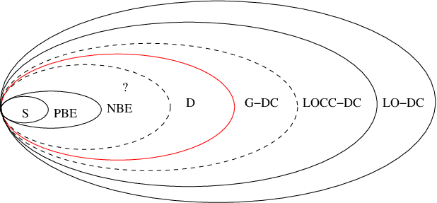
Although the classification above into S, PBE, NBE, D, and G-DC was considered for a multiparty state, this is essentially the classification for bipartite states. This classification is summarized in Fig. 1, where for the bipartite case, only the classes S, PBE, NBE, D, and G-DC are meaningful. The multiparty case offers a much richer classification: the states $\rho^{A_{1}\cdots A_{N}B_{1}B_{2}}$ that are distillable in the $A_{1}\cdots A_{N}:B_{1}B_{2}$ split, can in this case be divided into the following four classes:

1. 1.

   LO-DC class: This class contains states that can be used for dense coding even when the Bobs are separated and they do not even communicate classically. Precisely, they are those for which

   $$C_{LO}>\log_{2}d_{A_{1}}+\log_{2}d_{A_{2}}+\cdots+\log_{2}d_{A_{N}},$$

   (25)

   i.e. for which $S(\rho^{B_{1}})+S(\rho^{B_{2}})>S(\rho^{A_{1}A_{2}\cdots A_{M}B_{1}})+S(\rho^{A_{M+1}A_{M+2}\cdots A_{N}B_{2}})$.

2. 2.

   LOCC-DC class: This class contains states that are useful for dense coding when the two Bobs are separated, but they are allowed to communicate classically. So, these are states for which

   $$C_{LOCC}>\log_{2}d_{A_{1}}+\log_{2}d_{A_{2}}+\cdots+\log_{2}d_{A_{N}}.$$

   (26)

   Moreover, we require that the states in the LOCC-DC class to be not LO-DC.

3. 3.

   G-DC class: This class contains states that are useful for dense coding when the two Bobs are at the same location. Therefore, for these states

   $$C_{G}>\log_{2}d_{A_{1}}+\log_{2}d_{A_{2}}+\cdots+\log_{2}d_{A_{N}}.$$

   (27)

   Again we also require that the states in the G-DC class are not LOCC-DC.

4. 4.

   D class: The final class contains the states that are distillable in the $A_{1}A_{2}\cdots A_{N}:B_{1}B_{2}$ split, but not G-DC:

   $$C_{G}\leq\log_{2}d_{A_{1}}+\log_{2}d_{A_{2}}+\cdots+\log_{2}d_{A_{N}}.$$

   (28)

In this paper, we have introduced dense coding protocols for multipartite states where all the parties are far apart. We have considered two types of schemes: one with several senders and a single receiver, and another with several senders and two receivers who are allowed to perform only local operations. In the first case, we found the exact capacity of the channel while in the latter case, we provide a useful upper bound. In the latter case, we have also shown that the GHZ state achieves the upper bound. These two protocols help us to classify multipartite states from the point of view of usefulness for dense coding. In the bipartite case, this classification is complete. We know that separable states as well as bound entangled states are not useful for dense coding, while highly distillable states are good for it. There exist some distillable states which are not useful for dense coding. However in the multipartite situation, several questions remain open, both for one and two receiver(s). For example, we do not know whether multipartite bound entangled states are useful in such schemes. Let us consider the “unlockable” bound entangled state

of Ref. [32], where the $|\psi_{i}\rangle$s are the Bell states. Let $\rho_{S}$ be shared between $A_{1}$, $A_{2}$, $B_{1}$, $B_{2}$. $\rho_{S}$ is separable in all two party by two party splittings, although it has one bit of entanglement in all one party by three party splittings. One can check by using Eq. (23) that the $C_{G}$ of $\rho_{S}$ is not greater than 3 bits, but exactly equal to 3 bits, when $A_{1}$, $A_{2}$, $B_{1}$ are senders and $B_{2}$ is the receiver. Since all its two party by two party splittings are separable, it is clear that it will never be useful for dense coding with two receivers. We have also checked our formulas for other bound entangled states, e.g. the bound entangled states formed from the unextendible product bases [33], and they are not useful for dense coding either.

In this paper, we have considered distributed communication protocols, where the senders are only allowed to perform unitary operations. This case is more interesting from the perspective of a real implementation. However the Holevo-like upper bound [13] on accessible information holds for any encoding (as well as decoding) operation. So, it is also interesting to consider general encoding protocols, and obtain upper bounds on distributed communication rates in this case. For the latest development of this general case in a situation, where there is only a single sender and a single receiver, see e.g. [5, 6]. In this paper, it is always assumed that the transmission channel is noiseless, even if the shared states that we use as our resource may be noisy. Even in the case of such noiseless channels, we show that the states that we require in such communication are highly entangled. It would be interesting to study the dense coding capacity of noisy states in the realistic case of noisy channels.

We thank Alexander Holevo and Mario Ziman for valuable comments. We acknowledge support from the Deutsche Forschungsgemeinschaft (SFB 407, SPP 1078, SPP 1116, 436POL), the Alexander von Humboldt Foundation, the EC Program QUPRODIS, the ESF Program QUDEDIS, and EU IP SCALA.

References

- [1] C.H. Bennett et al., Phys. Rev. Lett. 70, 1895 (1993).
- [2] C.H. Bennett and S.J. Wiesner, Phys. Rev. Lett. 69, 2881 (1992).
- [3] C.H. Bennett et al., Phys. Rev. Lett. 83, 3081 (1999).
- [4] C.H. Bennett et al., Entanglement-assisted capacity of a quantum channel and the reverse Shannon theorem, quant-ph/0106052.
- [5] M. Horodecki et al., Q. Inf. and Comput. 1, 70 (2001).
- [6] A. Winter, J. Math. Phys. 43, 4341 (2002).
- [7] S. Bose, M.B. Plenio, and V. Vedral, Mixed state dense coding and its relation to entanglement measures, quant-ph/9810025.
- [8] T. Hiroshima, J. Phys. A: Math. Gen. 34, 6907 (2001).
- [9] M. Ziman and V. Bužek, Phys. Rev. A 67, 042321 (2003).
- [10] X.S. Liu et al., Phys. Rev. A 65, 022304 (2002).
- [11] D. Bruß et al., Phys. Rev. Lett. 93, 210501 (2004).
- [12] J.P. Gordon, in Proc. Int. School Phys. “Enrico Fermi, Course XXXI”, ed. P.A. Miles, pp. 156 (Academic Press, NY 1964); L.B. Levitin, in Proc. VI National Conf. Inf. Theory, Tashkent, pp. 111 (1969); A.S. Holevo, Probl. Pereda. Inf. 9, 3 1973 [Probl. Inf. Transm. 9, 110 (1973)].
- [13] P. Badzia̧g et al., Phys. Rev. Lett. 91, 117901 (2003).
- [14] M. Horodecki, A. Sen(De), and U. Sen, Quantification of quantum correlation of ensemble of states, quant-ph/0310100.
- [15] T. M. Cover and J. A. Thomas, Elements of Information Theory (Wiley, 1991).
- [16] R. Josza, D. Robb, and W.K. Wotters, Phys. Rev. A, 49, 668 (1994).
- [17] B. Schumacher et al., Phys. Rev. Lett. 76, 3452 (1996).
- [18] M Horodecki et al., Phys. Rev. Lett. 93, 170503 (2004) .
- [19] B. Schumacher and M.D. Westmoreland, Phys. Rev. A 56, 131 (1997); A.S. Holevo, IEEE Trans. Inf. Theory 44, 269 (1998).
- [20] M. Horodecki, P. Horodecki, and R. Horodecki, Phys. Rev. Lett. 80, 5239 (1998).
- [21] M. Horodecki and P. Horodecki, Phys. Rev. A 59, 4206 (1999); N.J. Cerf, C. Adami, and R.M. Gingrich, ibid. 60, 898 (1999).
- [22] K.G.H. Vollbrecht and M.M. Wolf, Conditional entropies and their relation to entanglement criteria, quant-ph/0202058.
- [23] T. Hiroshima, Phys. Rev. Lett. 91, 057902 (2003).
- [24] A. Sen(De), U. Sen, and M. Lewenstein, Lower Bound on Locally Accessible Information: Local Subentropy, quant-ph/0505137.
- [25] D. P. DiVincenzo et al., Phys. Rev. A 61, 062312 (2000); W. Dür et al., Phys. Rev. A 61, 062313 (2000).
- [26] R.F. Werner, Phys. Rev. A 40, 4277 (1989).
- [27] D.M. Greenberger, M.A. Horne, and A. Zeilinger, in Bell’s Theorem, Quantum Theory, and Conceptions of the Universe, ed. M. Kafatos, (Kluwer, Dordrecht, 1989).
- [28] F. Verstraete et al., Phys. Rev. A 65, 052112 (2002).
- [29] P.W. Shor, J.A. Smolin, and B.M. Terhal, Phys. Rev. Lett. 86, 2681 (2001).
- [30] T. Eggeling et al., Phys. Rev. Lett. 87, 257902 (2001).
- [31] A. Wehrl, Rev. Mod. Phys. 50, 221 (1978).
- [32] J.A. Smolin, Phys. Rev. A 63, 032306 (2001).
- [33] C.H. Bennett et al., Phys. Rev. Lett. 82, 5385 (1999); D.P. DiVincenzo et al., Comm. Math. Phys. 238, 379 (2003).