Generation of generalized coherent states with two coupled Bose-Einstein condensates.

Combined advances in evaporative cooling techniques and magneto-optical trapping made it possible to create an atomic Bose-Einstein Condensate (BEC) experimentally, an important achievement of the last decade. Initially predicted by Einstein in 1925 Einstein 1925, it was produced in 1995 from a dilute gas of rubidium atoms Anderson et al. 1995. Other research groups produced condensates using sodium Davis et al. 1995, lithium Bradley et al. 1997 and hydrogen Fried et al. 1998. In a second generation of experiments, it was shown to be possible to create double condensates. Such a system can be constructed by trapping atoms in two different hyperfine sublevels of ⁸⁷Rb Myatt et al. 1997; Matthews et al. 1998.

Measurements of scattering lengths Hall et al. 1998a and research on the dynamics of the relative phase of the condensates Hall et al. 1998b and Rabi oscillations of the two BEC populations Matthews et al. 1999, can be carried out by using a laser-induced Raman transition in the ⁸⁷Rb experimental setup. The experimental production of the first BEC and the analogy between the behavior of the coherent matter waves and the electromagnetic ones, encouraged the development of Atom Optics Anderson and Meystre 2003. Nowadays, quantum optics tools are commonly used in the study of the BEC properties. Another consequence of this analogy is the study of problems already explored in quantum optics but mapped into the context of atomic systems. One example is the generation of “Schrödinger cat”-like states (SCS) whose creation in quantum optics via dynamical procedures involving nonlinear interaction, was proposed by Yurke and Stoler Yurke and Stoler 1986 and discussed by several authors Gerry et al. 2002; Gerry 1999; Agarwal et al. 1997; Agarwal and Banerji 1998. These schemes involve Kerr-like couplings and, in general, coherent states are used as initial states.

When two coupled BECs are analyzed by using a many-body Hamiltonian within the two-mode approximation (TMA), the terms that describe atomic collisions are analogous to a Kerr-like interaction Milburn et al. 1997. An additional Raman transition could be switched on so there is a Josephson-like coupling between the two modes. In this case, each mode corresponds to one of the BEC species and it is necessary to take into account inter- and intraspecies scattering processes. TMA was used by several authors to explore the possibility of creating quantum superposition states in BECs Cirac et al. 1998; Gordon and Savage 1999. Cirac et al. Cirac et al. 1998 calculated the ground state of the TMA Hamiltonian for various choices of coupling parameters. For certain sets of parameter values, the ground state is a SCS. Gordon and Savage Gordon and Savage 1999, among others, proposed the generation of SCS by exploiting the dynamical evolution of the system, in a similar fashion as has been done in the electromagnetic waves Yurke and Stoler 1986. Other aspects of BECs recently studied are the entanglement dynamics and the generation of entangled states Sørensen et al. 2001; You 2003; Micheli et al. 2003; Hines et al. 2003. A dynamical scheme was proposed by Micheli et al. Micheli et al. 2003 in order to generate a many-particle entangled state. In their approach, the entangled subsystems correspond to the individual atoms in BECs.

In the present contribution, we propose the generation of the Generalized Coherent State (GCS) in a system with two coupled BECs. The GCS was introduced by Titulaer and Glauber Titulaer and Glauber 1966 as a generalization of Glauber’s coherent state, defined as

Here, the phases $\upsilon_{m}$ are functions of index $m$ which ensures Poisson excitation statistics. For the periodic case, when $\upsilon_{m+l}=\upsilon_{m}$, GCS can be written as a superposition of $l$ coherent states with equal mean value of excitation $\left|\gamma\right|^{2}$ Bialynicka-Birula 1968:

Within the TMA we determine the conditions at wich two BECs, starting as a product of coherent states, first become entangled and, later, at certain specific times evolve to a product of the vacuum state and a GCS. We also show that the phases $\upsilon_{m}$ of the created GCS are periodic, and hence it can be rewritten as a superposition of $l$ coherent states. The period $l$ is fixed by both, the Josephson-like and nonlinear coupling strengths. We also explore numerically the dynamics of the system with the same initial state, in which the interspecies collision process is gradually inhibited. In these situations an exact GCS in no longer attained, but the evolved state has interesting properties such as sub-Poisson statistics, at the time GCS would have formed.

The paper is structured as follows. In Sec. II, we review the two-mode approximation, defining the parameters of interest in our calculation. Section III is reserved for the analysis of the necessary conditions to obtain a pure GCS. Also, we analyze the possibility of controlling the number of coherent states in the created superposition, by changing the coupling strengths. We estimate the evolution time necessary for the formation of the GCS. Section IV is devoted to the discussion of feasibility and sources of decoherence. Section V contains a numerical calculation of the dynamics of the system when the collisions between atoms of different species of BECs are inhibited. In Section VI, we summarize our results.

Our system consists of two atomic BECs of different atomic species labeled with suffixes $a$ and $b$, in a harmonic trap characterized by potentials $V_{a,b}\left(r\right)$. Interaction between atoms $a$ and $b$ are well described if we assume only two-body collisions. This can be done by considering three different scattering processes: $a-a$, $b-b$ and $a-b$ atomic collisions. We are interested in the dynamics of this system when Josephson-like coupling between species $a$ and $b$ of BECs is switched on. The second quantized Hamiltonian which describes our system is given by Milburn et al. 1997; Cirac et al. 1998; Steel and Collett 1998; Villain and Lewenstein 1999

where

and $j=a,b$. Here, we have omitted spatial dependence in quantum field operators, $\hat{\Psi}_{a,b}$ ($\hat{\Psi}^{\dagger}_{a,b}$), which annihilate (create) atoms at position r. $m$ is the atomic mass and $\hat{V}_{a,b}\left(\textbf{r}\right)$ are the harmonic trap potentials and $A_{a,b}$ are the scattering lengths associated with collisions between atoms of the same condensate (intraspecies collisions). Hamiltonian $\hat{H}_{ab}$ describes the interaction between atoms of different species due to two-body collisions (interspecies collisions). $H_{\mbox{c}}$ is the Josephson-like coupling between the modes, $\delta$ being the detuning from Raman resonance and $\Omega$ is the Rabi frequency.

Following a procedure similar to that described in Ref. Cirac et al. 1998, we obtain the TMA Hamiltonian. The field operators are written as $\hat{\Psi}_{a}=\phi_{a}\left(\textbf{r}\right)\hat{a}$ and $\hat{\Psi}_{b}=\phi_{b}\left(\textbf{r}\right)\hat{b}$, $\phi_{a,b}\left(\textbf{r}\right)$ being the real spatial functions associated with each mode and $\hat{a}$ and $\hat{b}$ the standard bosonic operators. Additionally, we consider here $\delta=0$, to obtain the total Hamiltonian given by

with

The TMA Hamiltonian (6) can be used in the description of two different experimental situations. The first one is the condensation of sodium, where atoms condense in hyperfine states localized in two different minima of the harmonic trap Andrews et al. 1997; Stenger et al. 1998. In this case, Josephson-like coupling describes tunneling. In some cases, a good approximation is obtained by neglecting the interspecies collisions. However, it is more general to assume that $U_{ab}<U_{aa}=U_{bb}$.

The second situation is connected with the experiments of the JILA group with condensation of atoms on two different hyperfine ⁸⁷Rb levels. In this context, the Josephson-like coupling is associated with a laser-induced Raman transition between the hyperfine levels. Reported scattering length values follow the relation $A_{a}:A_{ab}:A_{b}\equiv 1.03:1:0.97$ Hall et al. 1998a; Hall et al. 1998b. From Eqs.(7b) and (7c) it is clear that parameters $U_{ij}$ obey the same relations, for a fixed spatial mode function $\phi_{a,b}\left(\textbf{r}\right)$. The latter is an important condition if we want to use the TMA: as we can see from Eqs.(7), the values of the strengths of the Hamiltonian depend on the spatial mode functions $\phi_{a,b}\left(\textbf{r}\right)$. The approximation is valid only if these functions remain unaltered and the parameters in each term of Hamiltonian (6) can be considered as constants ¹¹ 1 An estimative of validity of two-mode model can be found in Ref. Milburn et al. 1997. Also, in Section V of Ref. Gordon and Savage 1999, the authors discuss the different regimes in which this approximation is valid.. Several authors use $A_{a}=A_{b}=A_{ab}$ to simplify theoretical calculations with the Hamiltonian (2) Park and Eberly 2000; Villain and Lewenstein 1999. In the TMA Hamiltonian (6), this situation corresponds to $U_{ab}=U_{aa}=U_{bb}$.

In this article, we assume that $U_{aa}+U_{bb}=2U_{ab}$ in order to extend the analytical solution of the Schrödinger equation in L. Sanz et al. 2003 and show how the GCS is exactly generated. Notice that this assumption applies for both cases: equal scattering lengths approximation ($U_{aa}=U_{ab}=U_{bb}$) and for the relation between experimental measured scattering lengths ($U_{aa}:U_{ab}:U_{bb}\equiv 1.03:1:0.97$). Then, using numerical calculations, we explore the situation when $U_{ab}<U=U_{aa}=U_{bb}$. In this way, we are able to study the effect of the interspecies collision term on the dynamics and the transition between two different situations which can be related to the experimental contexts of rubidium and sodium ($U_{ab}\approx 0$) condensates.

In this section, we show how the dynamical evolution associated with the TMA Hamiltonian can be exploited to produce a product of the vacuum state and the GCS. We first assume, reasoning by analogy with BECs in optical lattices Greiner et al. 2002a, that the system could be prepared as a product of coherent states $\left|\Psi(0)\right>=\left|\alpha_{a}\right>\otimes\left|\alpha_{b}\right>$ where $\alpha_{j}$ are the amplitude of the state thus $\left|\alpha_{j}\right|^{2}$ is the atomic population on mode-$j$. It is demonstrated Greiner et al. 2002a that the manipulation of the Josephson-like coupling, by changing the potential depth between the $\ell$ local minima of the lattice, produces the state $\prod_{\ell}\left|\alpha_{\ell}\right>$. Another reason is that the coherent state satisfies the conditions for full coherence. In experiments, interference patterns between two BECs were observed Andrews et al. 1997 and collision-rate measurements Burt et al. 1997 probed the existence of third-order correlations. Although similar patterns could be obtained if BEC state is described either as Fock or coherent states You 2003; Castin and Dalibard 1999; Javanainen and Yoo 1996, studies about decoherence process due to three-body losses Jack 2002 supports the assumption that the state of a BEC is a coherent state with a well-defined phase. Also, phase and spatial dynamics were explored including the effect of fluctuations by Sinatra and Castin Sinatra and Castin 2000 and Ref. Villain and Lewenstein 1999. Results which are in agreement with the measure of relative phase between coupled condensate Hall et al. 1998b were obtained by Li et al. Li et al. 2001 considering the initial state $\left|\alpha_{a}\right>\otimes\left|\alpha_{b}\right>$.

In this work we shall focus on the macroscopic superposition state resulting from the evolution of the system itself. Solving the Schrödinger equation associated with Hamiltonian (6), as shown in the Appendix A, the evolved state ($\hbar=1$) is given by

with

and

being $N$ the total excitation number of the system, which is a constant of motion and $\lambda_{1}$ the effective Rabi frequency.

We see that the state represented by Eq.(8) is an entangled state and there are only two situations where $\left|{\psi\left(t\right)}\right>$ can be written as a direct product: The first is when the interaction parameter $U_{ab}t$ is a multiple of $\pi$ and the function $\exp{\left(-2inmU_{ab}t\right)}$ in Eq.(8) is equal to unity. Thus, the disentanglement times associated with this first condition depend only on the value of the nonlinear coupling strength $U_{ab}$. At these times, $\left|\psi\left(t\right)\right>$ can be rewritten as a direct product of new coherent states. The second case arises at those times such that either $\alpha\left(t\right)$ or $\beta\left(t\right)$ is zero, and the evolved state can be written as a product of the vacuum state and a superposition of Fock states.

The creation of the GCS given by Eq.(11) is restricted to the times associated with the second situation: if, for example, at certain evolution time $t_{e}$ the quantity $\alpha(t_{e})=0$, the evolved state can be written as

Therefore, the GCS is a special superposition of Fock states and obeys Poisson statistics. From Eqs.(9a) and (9b) we conclude that the condition when either $\alpha\left(t\right)$ or $\beta\left(t\right)$ is zero can be written as

with $i\neq j=a$ or $b$, depending on which quantity, $\alpha(t)$ or $\beta(t)$ goes to zero. Next, we analyze two particular choices of the interaction parameter, $\lambda_{1}t_{e}$, leading to the GCS:

1. 1.

   At times given by

   $$\lambda_{1}t_{p}=\frac{2p+1}{4}\pi$$

   (13)

   where $p$ is a positive or zero integer, the initial states satisfy the relation

   $$\alpha_{i}=\frac{1}{\lambda}\left(\pm\omega_{1}+i\lambda_{1}\right)\alpha_{j}.$$

   (14)

   Note that in the particular case $\omega_{a}=\omega_{b}$ and $U_{aa}=U_{ab}=U_{bb}$ Park and Eberly 2000; Villain and Lewenstein 1999, we obtain, from Eqs.(10b) and (10c), that $\omega_{1}=0$ and $\lambda_{1}=\lambda$, and Eq.(14) is reduced to $\alpha_{j}=i\alpha_{i}$. Therefore, the initial mean number of atoms in each mode, $\langle\hat{n}_{a}\rangle$ and $\langle\hat{n}_{b}\rangle$, must be equal ($\left|\alpha_{a}\right|^{2}=\left|\alpha_{b}\right|^{2}$) with the relative phase $\Delta\phi=\phi_{a}-\phi_{b}$ corresponding to $\frac{\pi}{2}$.

2. 2.

   At times $\lambda_{1}t_{k}=k\pi$, we obtain the condition $\alpha_{j}=0$. Therefore, it is possible to generate the GCS if, for instance, initially all the $N$ atoms are condensed in the mode-$a$ and the second hyperfine level (mode-$b$) is used as an auxiliary mode. Thus, the atomic population leaves mode-$a$ and returns, not as a coherent state but as the GCS. For the initial state, $\left|\Psi(0)\right>=\left|\sqrt{N}\right>\otimes\left|0\right>$, we find that $\left|\Psi(t_{k})\right>=\left|\mbox{GCS}\right>_{N,0}\otimes\left|0\right>$ with

   	$\displaystyle\left|\mbox{GCS}\right>_{N,0}$	$\displaystyle=$	$\displaystyle e^{-\frac{N}{2}}\sum\limits_{n}\frac{\left[\sqrt{N}e^{-i\pi\frac{\omega_{0}}{\lambda_{1}}}\right]^{n}}{\sqrt{n!}}$		(15)
   			$\displaystyle\times e^{-ik\frac{U_{ab}}{\lambda_{1}}\pi n^{2}}\left|n\right>.$

   This particular case is interesting because it is possible to create the GCS without the necessity to “imprint” any initial phase relation between the coupled BECs.

It is possible to rewrite the GCS as a superposition of coherent states Bialynicka-Birula 1968 if the phases given by $\upsilon_{n}=U_{ab}t_{e}n^{2}$ on Eq.(11) are periodic. In our context, the necessary condition to obtain this kind of “Schrödinger cat”-like state is $U_{ab}t_{e}=r/s$, with $r$ and $s$ integers. This implies that the interspecies collision strength and effective Rabi frequency could also be written as a rational fraction. When this applies, we can use the discrete Fourier transform J. Banerji 2001 on Eq.(11). It is straightforward to rewrite $\left|\mbox{GCS}\right>$ as the superposition

where $l$ is the number of coherent states present in the superposition. This value is defined by the condition below

The coefficients $a_{m}^{\left(r,s\right)}$ have the form

We see that the GCS corresponds to a superposition of coherent states with the same mean excitation number ($|\beta|^{2}$) and relative phases equal to $e^{-2\pi i\frac{m}{l}}$. Note that the number of coherent states in the $\left|\mbox{GCS}\right>$ depends on the ratio of nonlinear $U_{ab}$ to effective Rabi frequency $\lambda_{1}$.

In Figure 1 we plot the Husimi quasi-distribution function at time $t_{e}=\frac{\pi}{4\lambda_{1}}$ for $\omega_{a}=\omega_{b}$ and $U_{aa}-U_{bb}\sim 10^{-2}U_{ab}$. When $U_{ab}$ and $\lambda_{1}$ are chosen such that $r/s=2/3$, we obtain three distinguishable packets as shown in Fig. 1(a). Modifying the $U_{ab}/\lambda_{1}$ ratio it is possible to achieve a superposition of any number of coherent states. For instance, if $U_{ab}/\lambda_{1}=8/5$ we obtain superpositions of five coherent states as shown in Fig. 1(b). If $U_{ab}/\lambda_{1}=1/2$, we obtain eight packages, Fig. 1(c). Superposition of nine coherent states, shown in Fig. 1(d), is obtained when coupling strengths are set such that $\frac{U_{ab}}{\lambda_{1}}=\frac{8}{9}$. The last plot shows that the different gaussian packets, associated with different coherent states in $\left|\mbox{GCS}\right>$, start to merge in phase space at high values of $l$. We also note that in Figs. 1(c-d) the deviation from a circular pattern of each gaussian packet in the superposition arises from interference between the packets, due to their proximity.

Because the effective Rabi frequency depends on the values of traps frequencies $\omega_{j}$ and collision parameters, all the examples above show that the formation of superpositions of coherent states in this scenario is highly sensitive to changes in these quantities and Josephson-like coupling. This means that, by controlling the values of scattering lengths, the effective harmonic potential, and the coupling between two species of condensates, it is possible to “build” a superposition of any desired number of coherent states, with a defined number of elements, mean excitation values and relative phases.

Next, we estimate the shortest time interval $t_{e}$ required to obtain the product state $\left|0\right>\otimes\left|\mbox{GCS}\right>$. The value of $t_{e}$ depends inversely on the effective Rabi frequency $\lambda_{1}$ ($t_{e}\varpropto\frac{\pi}{\lambda_{1}}$). First, we assume Gaussian spatial mode functions $\phi_{i}\left(\textbf{r}\right)$:

where $r_{0}=\sqrt{\hbar/2m\omega}$, being $\omega=\omega_{a}=\omega_{b}$. Then, using the typical physical parameters of Rubidium experiments, $\omega=50$ s^-1, $m=1.4\times 10^{-25}$ Kg and the Rabi frequency $\Omega\sim 2\pi\cdot 600$ s^-1 Hall et al. 1998a, we calculate the value of $\lambda_{1}$ from Eq.(10c). Thus, we obtain $t_{e}\approx 10^{-3}$ s. It is important to note that $t_{e}$ can be set as short as possible by varying the Rabi frequency, $\Omega$, of Raman transition.

There are several questions about the feasiblity of the CGS arising from the results above. The first one is how to set the system in a convenient initial state. From all the possibilities suggested by Eq.(12), we conclude that the most reasonable initial condition is $\left|\alpha_{a}\right>\otimes\left|0\right>$. This state describes a condensate (in $a$-mode) and an empty auxiliary level ($b$-mode) described as a vacuum state. In this situation, the imprint of a relative phase between a pair of coupled BECs is not necessary.

Second question is the necessity of an efficient atomic population transference. If decoherence affects the process, we cannot guarantee the formation of the state $\left|\mbox{GCS}\right>\otimes\left|0\right>$. Following Ruostekoski and Walls Ruostekoski and Walls 1998 the effects of decoherence due to noncondensed atoms on BECs shows that purity decays fast, being lower than $0.2$ at $U_{aa}t\approx 0.1$. Hence, one must have the interaction parameter $\lambda_{1}t$ much smaller than the decoherence time scale associated with $U_{aa}\sim U_{ab}$.

Once the GCS is created and Raman transition is switched off, it is necessary to check the effects of both, nonlinear interactions and decoherence. Because the fraction of noncondensed atoms is small, we can perform a simple calculation assuming that the interaction between those atoms and BEC induce phase-damping rather than atomic losses. Thus, we shall consider small the effect of decoherence due to condensate feeding and depleting. The following master equation for the density operator of $a$-mode, $\hat{\rho}_{a}$, applies Anglin 1997; Louis et al. 2001

with $H_{a}=\hbar\omega_{a}\hat{a}^{\dagger}\hat{a}+\hbar U_{aa}\hat{a}^{\dagger}\hat{a}^{\dagger}\hat{a}\hat{a}$. It is straightforward to calculate the solution of Eq.(19). They resemble the solutions for the phase-damped oscillator Gardiner and Zoller 2000:

If $\kappa=0$, we are able to study the dynamics associated with atomic intraspecies collisions (nonlinear interaction term in $\hat{H}_{a}$), assuming that we create successfully the GCS described by Eq.(15). From Eq.(20), the density matrix is given by

with

Nonlinear collisions do not affect the character of the state and BEC is still in a GCS, with time-dependent amplitude $\Upsilon(t)$ and phase $U(t)$. From the analysis of Sec. III, we note that superpositions shown in Fig.1 can be destroyed as time progresses due to the changes on function $U(t)$ defined in Eq.(22). The effect of nonlinear interaction after the creation of the GCS could be reduced by manipulation of scattering length $A_{a}$ through a Feshbach resonance Vogels et al. 1997: controlling the scattering length, it is possible to change the value of $U_{aa}t$ so $U(t)$ varies smoothly with time.

For $\kappa\neq 0$, we calculate $\mbox{Tr}\left[\hat{\rho}_{a}^{2}(t)\right]$ in order to quantify the effects of the reservoir of noncondensed atoms on the BEC. We plot this quantity in Fig. 2 for different choices of $\kappa$ and number of atoms. From this results it is clear that, for large values of $\kappa$ the state is no longer a GCS neither a pure state. Additionally, the decay rate is sensitive to changes on $\kappa$ and $N$, decaying faster when both quantities increase. Hence, the phase damping is a serious limitation for manipulation of the GCS. Another source of decoherence is the three-body losses. Measurements of density-dependent losses demonstrate that three-body recombination is the dominant decoherence mechanism, which limits the lifetime and size of BECs Burt et al. 1997. In order to study the decoherence process due the three-body losses, a master equation is derived by M. Jack Jack 2002, where it is shown that a coherent state is a robust state in the limit of large-number of atoms. However, it is also shown that the superpositions defined in Eq.(16) are sensitive to the three-body losses.

Last concern is the effect of temperature and the ratio between Josephson and nonlinear couplings. A careful study of this effects on dephasing process was performed by Pitaevskii and Stringari Pittaevskii and Stringari 2001. They shown that coherence is strongly dependent on the ratio between Josephson coupling and collisions strength, $U_{jj}/\lambda$ and also with temperature, $T/\lambda$. One must have control over both ratios to keep them small in order to keep the phase coherence.

In this section, we analyze the effect of the interspecies collisions on the dynamical evolution ($U_{ab}<U=U_{aa}=U_{bb}$). This is done by solving the Schrödinger equation numerically by direct diagonalization of the Hamiltonian (6) in a truncated Fock basis $\left\{|n_{a},n_{b}\rangle\right\}$. In order to compare the results for $U_{ab}<U$ with those obtained when the condition $U_{aa}+U_{bb}=2U_{ab}$ is considered, we set the initial states as $\left|\alpha_{a}\right|^{2}=\left|\alpha_{b}\right|^{2}$ with relative phase $\Delta\phi=\pi/2$. We calculate the fraction of the total atom population in mode $b$, $\langle\hat{n}_{b}\rangle/N=\langle\hat{b}^{\dagger}\hat{b}\rangle/N$, and its variance $\langle|\Delta\hat{n}_{b}|^{2}\rangle=\langle\hat{n}_{b}^{2}\rangle-\langle\hat{n}_{b}\rangle^{2}$. The “distance” between different states in the Fock basis can be analyzed using both $\langle|\Delta\hat{n}_{b}|^{2}\rangle$ and the variance of operator $\hat{b}$, defined as $\langle|\Delta\hat{b}|^{2}\rangle=\langle\hat{b}^{{\dagger}}\hat{b}\rangle-\langle\hat{b}^{{\dagger}}\rangle\langle\hat{b}\rangle$ Kist et al. 1999. This last relation is useful to determine whether a given state can be considered as an eigenvalue of $\hat{n}_{b}$ or $\hat{b}$. The Mandel parameter

and the linear entropy $S_{b}=1-\mbox{Tr}_{b}\left[\hat{\rho}^{2}_{b}\left(t\right)\right]$ are used, the first to characterize the statistics and the second to quantify the purity of the evolved state of mode $b$, respectively.

It is convenient to recall some well-known values for the definitions written above. For a coherent state ($\left|\alpha\right>$), associated with $\hat{b}$ and $\hat{b}^{\dagger}$ operators, we obtain

indicating a Poisson statistics and that $\left|\alpha\right>$ is an eigenstate of $\hat{b}$. For a Fock state, $\left|n\right>$, we obtain

indicating a sub-Poisson statistics and that $\left|n\right>$ is an eigenstate of the $\hat{n}_{b}$ operator. In order to compare these values with the numerical results, let us calculate the expressions above in the case of equal scattering lengths. Using the reduced density operator for mode $b$ extracted from Eq.(8), it is straightforward to obtain

Except for the Mandel parameter, which is time independent, all the functions depend on $\left|\beta\left(t\right)\right|^{2}$, which is the mean atom population in mode $b$, written as

where $\left|\alpha\left(t\right)\right|^{2}+\left|\beta\left(t\right)\right|^{2}=N$. From Eqs.(26), we can recover the result obtained from the analysis in Sec. III of the evolved state. The dynamics depends strongly on the relative phase and the initial population of both condensates. From the behavior of the partial population, $\langle\hat{n}_{b}\rangle$, assuming $\Delta\phi=0$ and $\left|\alpha_{a}\right|=\left|\alpha_{b}\right|$, we obtain $\left|\beta\left(t\right)\right|^{2}=\left|\alpha_{b}\right|^{2}$ and there is no transfer of population between the condensates. However, if $\Delta\phi=\pi/2$ we can see that $\langle\hat{n}_{b}\rangle=\left|\alpha_{b}\right|^{2}\left[1-\sin{\left(2\lambda t\right)}\right]$ and the system undergoes Rabi oscillations with period equals to $\pi/\lambda$.

We also observe that the variance $\langle|\Delta\hat{b}|^{2}\rangle$ is zero at times corresponding either to $\pi/U$ or when $\left|\beta\left(t\right)\right|^{2}$ goes to zero. Since the reduced linear entropy is also zero at these times, as we discussed in Sec.III, the variance $\langle|\Delta\hat{b}|^{2}\rangle$ indicates that mode $b$ is in a coherent state. The Poisson statistics remains as time passes, independently of the entanglement dynamics of both modes.

In Fig. 3, we analyze the evolution of the atomic fraction in mode $b$, $\langle\hat{n}_{b}\rangle/N$, the Mandel parameter $Q$ and the linear entropy, $\delta_{b}$, for decreasing values of interspecies collision strength. We also plot the dynamics of each variable associated with the condition of equal scattering lengths, shown by a solid gray line. The vertical thick gray line indicates the time scale for formation of a GCS, $t_{e}$. The first aspect to be noticed in Fig.3(a) is a shift in the effective Rabi frequency of $\langle\hat{n}_{b}\rangle/N$ oscillations with decreasing $U_{ab}$. Also, there is an attenuation of Rabi oscillations if we compare both cases $U_{ab}=U$ and $U_{ab}=0$, shown in the inset. In particular, there are times at which the transfer of population is suppressed and atoms in each condensate are trapped. This “self-trapping” phenomenon was discussed elsewhere Milburn et al. 1997. We want to point out that the self-trapping can be associated with inhibition of interspecies collision and it is found even at slight differences between $U$ and $U_{ab}$.

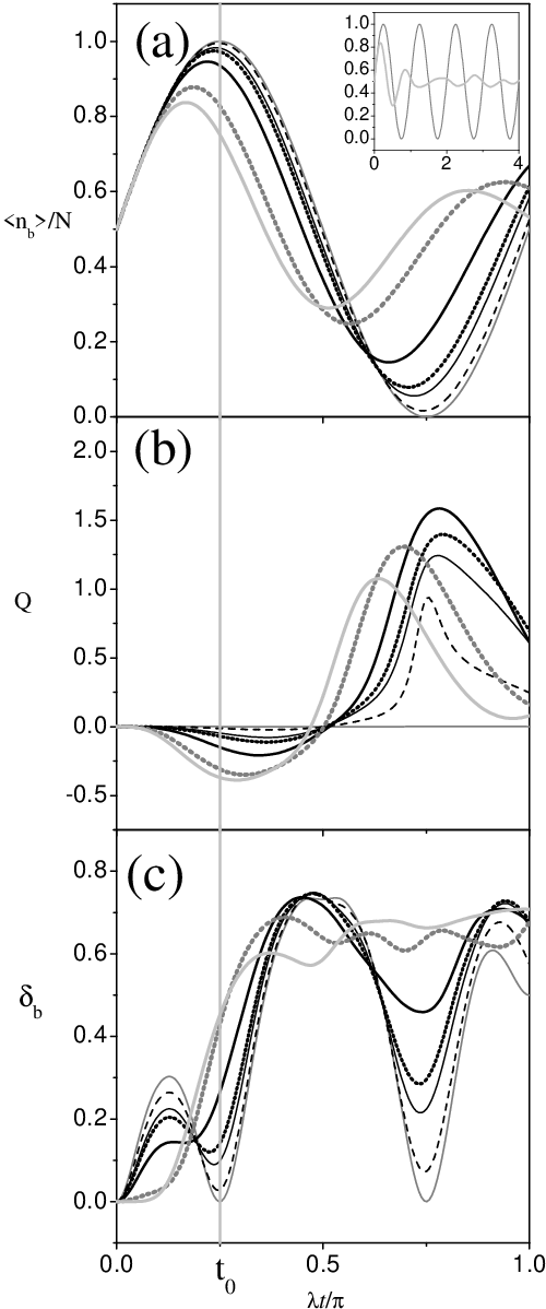
The dynamics of the Mandel parameter, Fig.3(b), shows that the subsystem state presents sub-Poisson statistics at short times, with $Q$ becoming more negative as $U_{ab}$ decreases. Super-Poisson statistics are obtained at later times. Our results show that an appropriate manipulation of $U_{ab}$ leads the initial coherent state to a new one, with sub or super-Poisson statistics depending on the evolution time. It is interesting to note that, for $U_{ab}=0$, the time necessary to reach the minimum of Mandel parameter $Q$ is almost the same as that of the formation of GCS.

From our results for $S_{b}$, Fig. 3(c), we see that the entanglement process is now irreversible. A small change of $U_{ab}$ produces an increase in the linear entropy and the subsystems are unable to recover purity. In view of this result, we conclude that slight changes in our conditions for generation of the GCS destroys such a state. The variance of $\hat{b}$ operator is shown in Fig. 4, for the same values of $U_{ab}$ as in Fig. 3. In all cases, there are no times at which $\langle|\Delta\hat{b}|^{2}\rangle=0$, as in the case of equal scattering lengths, and mode $b$ never returns to a coherent state.

At this point, it is worth recalling that in the sodium condensate, $\lambda$ is associated with the tunnelling frequency between the two minima of potential, which depends on the width of the barrier. We can assume the values used by Milburn et al. in order to check the time scales in this case. With $U$ approximately $53$ s^-1 and $\lambda\sim 0.37\times 10^{3}$ s^-1, we estimate $T_{U}\sim 6\times 10^{-2}$ s and $t_{e}\sim 2\times 10^{-3}$. Again, the time scales for the formation of states with sub-Poisson statistics is of the order of milliseconds and shorter than the time scale associated with the internal collisions.

Using the TMA Hamiltonian for the description of two coupled Bose-Einstein condensates, we demonstrate the possibility of creating a generalized coherent state in one of the condensate modes. The procedure presented here implies only dynamical evolution and requires the preparation of BECs in coherent states, which must follow the condition given by Eq.(12). The time necessary to obtain such a state depends only on the effective Rabi frequency $\lambda_{1}$, which is a function of Hamiltonian parameters. Also, it is shown that the ratio between the collision parameter $U_{ab}$ and $\lambda_{1}$ defines the number of coherent states contributing to the GCS. For $U_{ab}<U_{aa}=U_{bb}$, a new kind of non-classical statistics state is created. The analysis of fractional population, Mandel parameter and variance of the annihilation operator $\hat{b}$ shows some interesting dynamical effects associated to this state. Such effects are, for instance, a shift of the effective Rabi frequency, some temporal regimes with sub-Poisson and super-Poisson statistics and irreversible entanglement.

References

- Einstein (1925) A. Einstein, Siltzungsber. K. Preuss. Akad. Wiss., Phys. Math. Kl. 261 (1925).
- Anderson et al. (1995) M. H. Anderson, J. R. Ensher, M. R. Matthews, C. E. Wiemann, and E. A. Cornell, Science 269, 198 (1995).
- Davis et al. (1995) K. B. Davis, M. O. Mewes, M. R. Andrews, N. J. V. Druten, D. S. Durfee, D. M. Kurn, and W. Ketterle, Phys. Rev. Lett. 75, 3969 (1995).
- Bradley et al. (1997) C. C. Bradley, C. A. Sackett, and R. G. Hulet, Phys. Rev. Lett. 78, 985 (1997).
- Fried et al. (1998) D. G. Fried, T. C. Killian, L. Willmann, D. Landhuis, S. C. Moss, D. Kleppner, and T. J. Greytak, Phys. Rev. Lett. 81, 3811 (1998).
- Myatt et al. (1997) C. J. Myatt, E. A. Burt, R. W. Ghrist, E. A. Cornell, and C. E. Wieman, Phys. Rev. Lett. 78, 586 (1997).
- Matthews et al. (1998) M. R. Matthews, D. S. Hall, D. S. Jin, J. R. Ensher, C. E. Wieman, E. A. Cornell, F. Dalfovo, C. Minniti, and S. Stringari, Phys. Rev. Lett. 81, 243 (1998).
- Hall et al. (1998a) D. S. Hall, M. R. Matthews, J. R. Ensher, C. E. Wieman, and E. A. Cornell, Phys. Rev. Lett. 81, 1539 (1998a).
- Hall et al. (1998b) D. S. Hall, M. R. Matthews, C. E. Wieman, and E. A. Cornell, Phys. Rev. Lett. 81, 1543 (1998b).
- Matthews et al. (1999) M. R. Matthews, B. P. Anderson, P. C. Haljan, D. S. Hall, M. J. Holland, J. E. Williams, C. E. Wieman, and E. A. Cornell, Phys. Rev. Lett. 83, 3358 (1999).
- Anderson and Meystre (2003) B. Anderson and P. Meystre, Contemporary physics 44, 473 (2003).
- Yurke and Stoler (1986) B. Yurke and D. Stoler, Phys. Rev. Lett. 57, 13 (1986).
- Gerry et al. (2002) C. C. Gerry, A. Benmoussa, and R. Campos, Phys. Rev. A 66, 13804 (2002).
- Gerry (1999) C. C. Gerry, Phys. Rev. A 59, 4095 (1999).
- Agarwal et al. (1997) G. S. Agarwal, R. R. Puri, and R. P. Singh, Phys. Rev. A 56, 2249 (1997).
- Agarwal and Banerji (1998) G. S. Agarwal and J. Banerji, Phys. Rev. A 57, 3880 (1998).
- Milburn et al. (1997) G. J. Milburn, J. Corney, E. M. Wright, and D. F. Walls, Phys. Rev. A 55 (1997).
- Cirac et al. (1998) J. Cirac, M. Lewenstein, K. Mølner, and P. Zoller, Phys. Rev. A 57, 1208 (1998).
- Gordon and Savage (1999) D. Gordon and C. Savage, Phys. Rev. A 59, 4623 (1999).
- Sørensen et al. (2001) A. Sørensen, L. M. Duan, J. I. Cirac, and P. Zoller, Nature 409, 63 (2001).
- You (2003) L. You, Phys. Rev. Lett. 90, 030402 (2003).
- Micheli et al. (2003) A. Micheli, D. Jaksch, J. Cirac, and P. Zoller, Phys. Rev. A 67, 013607 (2003).
- Hines et al. (2003) A. P. Hines, R. H. McKensie, and G. J. Milburn, Phys. Rev. A 67, 013609 (2003).
- Titulaer and Glauber (1966) U. M. Titulaer and R. J. Glauber, Phys. Rev. 145, 1041 (1966).
- Bialynicka-Birula (1968) Z. Bialynicka-Birula, Phys. Rev. 173, 1207 (1968).
- Steel and Collett (1998) M. J. Steel and M. J. Collett, Phys. Rev. A 57 (1998).
- Villain and Lewenstein (1999) P. Villain and M. Lewenstein, Phys. Rev. A 59, 2250 (1999).
- Andrews et al. (1997) M. R. Andrews, C. G. Townsend, H. Miesner, D. S. Durfee, D. M. Kurn, and W. Ketterle, Science 275, 637 (1997).
- Stenger et al. (1998) J. Stenger, S. Inouye, D. M. Stamper-Kurn, H.-J. Miesner, A. P. Chikkatur, and W. Ketterle, Nature 396, 345 (1998).
- Park and Eberly (2000) Q.-H. Park and J. H. Eberly, Phys. Rev. Lett. 85 (2000).
- L. Sanz et al. (2003) L. Sanz, R.M. Angelo, and K.Furuya, J. Phys. A: Math. Gen. 36, 9737 (2003).
- Greiner et al. (2002a) M. Greiner, O. Mandel, T. Esslinger, T. Esslinger, T. W. Hänsch, and I. Bloch, Nature 415, 39 (2002a); M. Greiner, O. Mandel, T. W. Hänsch, and I. Bloch, Nature 419, 51 (2002b).
- Burt et al. (1997) E. A. Burt, R. W. Ghrist, C. J. Myatt, M. J. Holland, E. A. Cornell, and C. E. Wieman, Phys. Rev. Lett. 79, 337 (1997).
- Javanainen and Yoo (1996) J. Javanainen and S. M. Yoo, Phys. Rev. Lett. 76, 161 (1996).
- Castin and Dalibard (1999) Y. Castin and J. Dalibard, Phys. Rev. A 55, 4330 (1999).
- Jack (2002) M. W. Jack, Phys. Rev. Lett. 89, 140402 (2002); Phys. Rev. A 67, 043612 (2003).
- Sinatra and Castin (2000) A. Sinatra and Y. Castin, Eur. Phys. J. D 8, 319 (2000).
- Li et al. (2001) W.-D. Li, X. Zhou, Y. Wang, and W.-M. Liu, Phys. Rev. A 64, 015602 (2001).
- J. Banerji (2001) J. Banerji, PRAMANA- J. Phys. 56, 267 (2001).
- Ruostekoski and Walls (1998) J. Ruostekoski and D. F. Walls, Phys. Rev. A 58, R50 (1998).
- Anglin (1997) J. Anglin, Phys. Rev. Lett. 79, 6 (1997).
- Louis et al. (2001) P. J. Y. Louis, P. M. R. Brydon, and C. M. Savage, Phys. Rev. A 64, 053613 (2001).
- Gardiner and Zoller (2000) C. Gardiner and P. Zoller, Quantum Noise (Springer-Verlag,, Berlin, 2000), 2nd ed.
- Vogels et al. (1997) J. M. Vogels, C. C. Tsai, R. S. Freeland, S. J. J. M. F. Kokkelmans, B. J. Verhaar, and D. J. Heinzen, Phys. Rev. A 56, R1067 (1997).
- Pittaevskii and Stringari (2001) L. Pittaevskii and S. Stringari, Phys. Rev. Lett. 87, 180402 (2001).
- Kist et al. (1999) T. B. L. Kist, M. Orszag, T. A. Brun, and L. Davidovich, J. Opt. B:Quantum Semiclass. Opt. 1, 251 (1999).