Relaxation of Pseudo pure states : The Role of Cross-Correlations
Abstract
In Quantum Information Processing by NMR one of the major challenges is relaxation or decoherence. Often it is found
that the equilibrium mixed state of a spin system is not suitable as an initial state for computation and a definite initial
state is required to be prepared prior to the computation.
As these preferred initial states are non-equilibrium states, they are not stationary and are destroyed with time as the spin
system relaxes toward
its equilibrium, introducing error in computation. Since it is not possible to cut off the relaxation processes completely,
attempts are going on to develop alternate
strategies like Quantum Error Correction Codes or Noiseless Subsystems. Here we study
the relaxation behavior of various Pseudo Pure States and analyze the role of Cross terms between different relaxation
processes, known as Cross-correlation. It is found that while cross-correlations accelerate
the relaxation of certain pseudo pure states, they retard that of others.
I I. Introduction
Quantum information processing (QIP) often requires pure state as the initial state preskill; chuangbook. Shor’s prime
factorizing algorithm shor, Grover search algorithm grover are few examples. Creation of pure state in NMR is
not easy due to small gaps between nuclear magnetic energy levels and demands unrealistic experimental conditions like near absolute
zero temperature or extremely high magnetic field. This problem has been circumvented by creating a Pseudo Pure State (PPS).
While in a pure state all energy levels except one have zero populations, in a PPS all levels except one have equal
populations. Since the uniform background populations do not
contribute to the NMR signal, such a state then mimics a pure state. Several methods of
creating PPS have been developed like spatial averaging
cory97; cory98, logical labeling chuang97; chuang98; kavita00; kavita1, temporal averaging chuangtemp, spatially
averaged logical labeling
technique (SALLT) maheshpra01. However pseudo pure state, as well as pure states are not stationary and are destroyed with
time as the spin system relaxes toward equilibrium.
In QIP there are also cases where
one or more qubits are initialized to a suitable state at the beginning of the computation and are used as storage or memory qubits
at the end of the computation performed on some other qubitschuangdelay. In these cases it is important for memory qubits to be in the
initialized state till the time
they are in use since deviation from the initial state adds error to the output result. Since it is not possible to stop
decay of
a state which is away from equilibrium, alternate strategies like Quantum Error Correction qec, Noiseless
subspace ns1; ns2 are being tried. Recently Sarthour et al.quadrel has reported a detailed study of relaxation of pseudo
pure states and few other states in a quadrupolar system. Here we experimentally examine the lifetime of various pseudo pure states in
a weakly J-coupled two qubit system. We find that cross
terms (known as cross-correlation) between different pathways of relaxation of a spin can retard the relaxation of certain
PPS and accelerate that of others.
In 1946 Bloch formulated the behavior of populations or longitudinal magnetizations when they are perturbed from the
equilibrium bloch.
The recovery toward equilibrium is exponential for a two level system and for a complex system the recovery involves
several time constants redfield. For complex systems the von Neumann-Liouville equation von; abragam
describes mathematically the time evolution of the density matrix in the magnetic resonance phenomena.
For system having more than one spin
the relaxation is described by a matrix called the relaxation matrix whose elements are linear combinations of spectral densities, which
in turn are Fourier transforms of time correlation function anilreview of the fluctuations of the various interactions responsible
for relaxation. There exist several different mechanisms for relaxation, such as,
time dependent dipole-dipole(DD) interaction, chemical shift anisotropy(CSA), quadrupolar interaction and spin rotation interaction anilreview.
The correlation
function gives the time correlations between different values of the interactions. The final correlation function has two major parts,
namely the ‘Auto-correlation’
part which gives at two different times the correlation between the same relaxation interaction and the
‘Cross-correlation’ part which gives the time correlation between two different relaxation interactions. The mathematics of cross
correlation can be found in detail, in works of Schneider sch1; sch2, Blicharski blicharski and Hubbard hubbard.
Recently a few models have been suggested to study the decoherence of the quantum coherence, the off-diagonal elements in density matrix
zurek; cory03. It can be shown that in absence of r.f. pulses and under secular approximation
the relaxation of
the diagonal and the off-diagonal elements of the density matrix are independent redfield. Here we study the
longitudinal relaxation that is the
relaxation of the diagonal elements of the density matrix and the role of cross-correlations in it.
II II. Theory
II.1 A. The Pseudo Pure State (PPS) : In terms of magnetization modes
In terms of magnetization modes the equilibrium density matrix of a two spin system is given by cory98; abragam; ernstbook; jonesgate[Fig.1],
| (1) |
where and are gyro-magnetic ratios of the two spins and respectively. The density matrix of a general state can be written as,
| (2) |
which for the condition ===K, corresponds to the density matrix of a PPS given by cory98,
| (3) |
where, K is a constant, the value of which depends on the method of creation of PPS.
The first two terms in the right hand side in Eq.2 and Eq.3 are the single spin order modes for the first and second spin respectively while the last term is
the two spin order mode of the two spins cory98. Choosing properly the signs of the modes, the various PPS of a
two-qubit system are,
| (4) |
The relative populations of the states for different PPS are shown in Fig. 2. As seen in Eq.2, in PPS the coefficients of the all three modes are equal. On the other hand equilibrium density matrix does not contain any two spin order mode. To reach Eq.3 starting from Eq.1, the two spin order mode has to be created and at the same time the coefficients of all the modes have to be made equal.
II.2 B. Relaxation of Magnetization Modes
The equation of motion of modes M is given by anilreview,
| (5) |
where is the relaxation matrix and is the equilibrium values of a mode. For a weakly coupled two-spin system relaxing via mutual dipolar interaction and the CSA relaxation, the two dominant mechanism of relaxation of spin half nuclei in liquid state, the above equation takes the form,
where is the self relaxation rate of the single spin order mode of spin , is the self
relaxation rate of the two spin order mode of spin and , is the cross-relaxation (Nuclear Overhouser Effect,
NOE) rate between spins and and
is the cross-correlation term between CSA relaxation of spin and the dipolar relaxation between the spins and .
and involve only the
auto-correlation terms
and involves only the cross-correlation termsanilreview. Magnetization
modes of one order relaxes to other orders through
cross-correlation and in absence of it the relaxation matrix becomes block diagonal within each order. The relaxation of modes are
in general dominated by their self relaxation , but in case of samples having long , the cross-correlation terms become
comparable with self-relaxation and play an important role in relaxation of the spins.
The formal solution of Eq. 5 is given by,
| (16) |
As time evolution of various modes are coupled, a general solution of the above equation requires diagonalization of the relaxation matrix. However, in the initial rate approximation Eq.7 can be written (for small values of t=) as,
| (17) | |||||
| (18) |
This equation asserts that in the initial rate approximation (for low ), the decay or growth of a mode is linear with time and the initial slope is proportional to the corresponding relaxation matrix element. If the modes are allowed to relax for a longer time, their decay or growth deviates from the linear nature and adopts a multi-exponential behavior to finally reach the equilibriumanilreview.
II.3 C. Relaxation of Pseudo pure state
Let a two qubit system be in PPS at t=0.
| (19) |
After time t it will relax to,
| (20) |
where , and are the time dependent deviations of respective modes from their initial values. The deviation of the two spin order can be measured from spectrum of either spin. Eq.20 can also be written as,
| (21) |
The first term is the pseudo pure state with the coefficient decreasing in time while the other two terms are the excesses of the single spin order modes with coefficients increasing in time. For other pseudo pure states Eq.21 becomes,
| (22) | |||||
| (23) | |||||
| (24) |
In the initial rate approximation (using Eq.18) we obtain for the pps,
| (25) | |||||
| (26) | |||||
| (27) |
Let the coefficients of the PPS term and the two single spin order modes and in Eq.21 be called as , and respectively. Fig.3 schematically shows the time evolution of the coefficients , and for PPS. Any coefficient for any PPS at any instant, is simply the initial value plus the total deviation due to the auto and the cross-correlations. For example, for PPS at time , is ), where K is the initial value, and and are the deviations at due to auto-correlation and cross-correlation parts respectively.
II.3.1 (a) Contribution of auto-correlation terms to the deviation
Putting the values of the deviations of different modes obtained from Eq.(25-27) in Eq.(21-24), we obtain the contribution only of auto-correlation terms to the deviation from initial value of the coefficients , and under initial rate approximation (at t=) as,
| ; | |||||
| ; | |||||
| ; | |||||
| ; | (28) |
It is evident that in absence of cross-correlations the and PPS relax at the same initial rate since , and . However the same is not true for and PPS.
II.3.2 (b) Contribution of cross-correlation terms to the deviation
The contribution by the cross-correlation terms is given by,
| ; | |||||
| ; | |||||
| ; | |||||
| ; | (29) |
The important
thing is that the presence of cross-correlation can lead to differential relaxation of all PPS.
Positive cross-correlation rates and , slow down the relaxation of all the
three coefficients for
PPS since (),
while make the relaxation of
all three coefficients faster for
PPS since ().
For and PPS cross-correlations give a mixed effect since
()
and ().
As the contributions of the
auto-correlation part for and PPS are equal, we have monitored the relaxation behavior only of and
PPS to study the effect of cross-correlations.
For samples having long , where the cross-correlations becomes comparable with auto-correlation rates, the four PPS relax with four different rates and the difference increases with the increased value of the cross-correlation terms. The three coefficients , and (normalized to the equilibrium line intensities) in terms of proton and fluorine line intensities for PPS are,
| (30) |
and for PPS are,
| (31) |
where, and are intensities of the two proton transitions, when the fluorine spin is respectively in state and . Similarly and are intensities of two fluorine transitions corresponding to the proton spin being respectively in the state and , as shown in Fig.1 and Fig.6. and give the line intensity respectively at time t and at equilibrium. Thus by monitoring the intensities of the two proton and two fluorine transitions as a function of time, one can calculate the coefficient which is a measure of decay of PPS.
III III. Simulation
Relaxation of the coefficients , and have been simulated using MATLAB, for a weakly coupled - system. The relaxation matrix used for the simulation is,
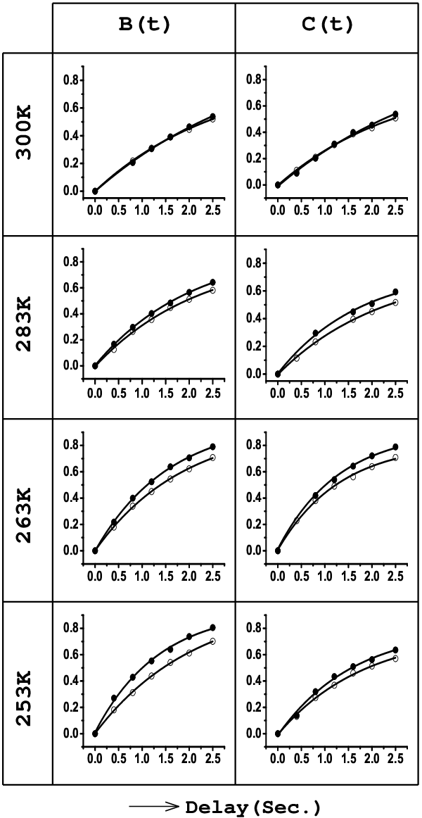
Fig.4 shows the decay of coefficient with time. and show no difference in decay rate in absence of cross-correlation rates. As and are increased more and more difference in decay rate is observed. Fig.5 shows growth of coefficients and . As is taken smaller than , difference in decay rate between and is found to be less than between and .
IV IV. Experimental
All the relaxation measurement were performed on a two qubit sample formed by one fluorine and one proton of 5-fluro 1,3-dimethyl uracil
yielding an AX spin system with a J-coupling of 5.8 Hz.
Longitudinal relaxation time constants for and are 6 and 7.2 Sec respectively at room temperature (300K). All the experiments were performed in a Bruker DRX 500 MHz spectrometer where the resonance frequencies for
and are 470.59 MHz and 500.13 MHz respectively. The Pseudo-pure
state was prepared by spatial averaging method
using J-evolution cory98.
Relaxation of all the three
coefficients for and PPS has been calculated. Since auto-correlations contribute equally to the
relaxation of
these two PPS, any difference in relaxation rate can be attributed to cross-correlation rates.
Sample temperature was
varied to change the correlation time and hence the cross-correlation rate . Four different sample
temperatures, 300K, 283K, 263K and 253K were used. Fig.6 shows the proton and fluorine spectra obtained using recovery
measurement at four different temperatures. The spectra correspond to the initial PPS state and that after an interval of
2.5 sec. Fig.7 shows the longitudinal relaxation times () of fluorine and
proton as function of temperature obtained from initial part of inversion-recovery experiment. A steady decrease in with decreasing temperature
indicates that the dynamics of the
sample molecule is in the short correlation time limit abragam. In this limit auto as well as cross-correlations increase
linearly with decreasing temperature.
All the spectra were fitted to bi-Lorentzian lines in MATLAB and various parameters were extracted using the Origin software. Fig.8 shows the decay of the coefficient calculated independently from proton and fluorine spectra. At 300K, and showed almost same rate of decay. As the temperature was gradually lowered, a steady increase in difference in decay rate was observed. This is due to the steady increase in cross-correlation rates with decreasing temperature, which is expected in the short correlation time limit. In Fig.9 the growths of the coefficients and are shown. Similar to the coefficient , coefficients and also show differences in decay rate between and PPS at lower temperatures. The difference between and at any temperature was found to be larger compared to between and . This is expected since, according to Eq.29 the dominant cross-correlation factor in and is which is the cross-correlation between CSA of fluorine with fluorine-proton dipolar interaction whereas in and the dominant factor is which is cross-correlation between CSA of proton, which is much less than fluorine, with fluorine-proton dipolar interaction. Thus it is found that at lower temperatures the PPS decays slower than the PPS. The dominant difference in the decay rates arises from the cross-correlations between the CSA of the fluorine and the dipolar interaction between the fluorine and the proton spin. To the best of our knowledge this is the first study of its kind where the differential decay of the PPS has been attributed to cross-correlations.
V V. Conclusion
We have demonstrated here that in samples having long cross-correlations plays an important role in determining the rate of relaxation of pseudo pure state. In QIP sometimes one or more qubits having comparatively longer longitudinal relaxation are used as storage or memory qubits. Recently Levitt et al. have demonstrated a long living antisymmetric state arrived by shifting the sample from high to very low magnetic field, suggesting that this long living state could be used as memory qubit levitthigh; levittlow. In such cases fidelity of computation depends on how much the memory qubits have been deviated from the initialized state at the beginning of the computation till the time they are actually used. Theoretically it is shown here that in presence of cross-correlations, all the four PPS relax with different initial rates. For positive cross-correlations the PPS relaxes significantly slower than PPS. It is therefore important to choose a proper initial pseudo pure state according to the sample.
Acknowledgments
We gratefully acknowledge Prof. K. V. Ramanathan for discussions and Mr. Rangeet Bhattacharyya for his help in data processing. The use of DRX-500 high resolution liquid state spectrometer of the Sophisticated Instrument Facility, Indian Institute of Science, Bangalore, funded by Department of Science and Technology (DST), New Delhi, is gratefully acknowledged. AK acknowledges ”DAE-BRNS” for ”Senior Scientist scheme”, and DST for a research grant.
FIGURE CAPTIONS
Figure 1. (a) Chemical structure of 5-fluro 1,3-dimethyl uracil. The fluorine and the proton spins (shown by circles) are
used as the two qubits and respectively. (b) The energy level diagram of a two qubit system identifying the four states 00,01,10 and 11. Under high temperature and high
field approximation abragam the relative equilibrium deviation populations are indicated in the bracket for each level. Assuming
this to be a weakly coupled two spin system the deviation populations become proportional to the gyromagnetic ratios and
. refers to the transition of the spin when the other spin is in state
. Thus means the proton transition when the
fluorine is in state .
Figure 2. Population distribution of different energy levels of a two spin system in different pseudo-pure states. K is a constant whose
value depends on the protocol used for the preparation of PPS. (a),(b),(c) and (d) show respectively the ,, and
PPS.
Figure 3. Schematic representation of decay of the coefficient and growth of the coefficients and . The magnetization modes
are normalized to their respective equilibrium values. In each sub-figure the three bars correspond to the modes , and
2 from left to right. The amount of any mode present at any time is directly proportional to the height of the corresponding
bar. The numbers provided in the rightmost column represent typical values of the modes. (a) Thermal equilibrium. At thermal equilibrium
only and exist. (b) pseudo-pure state
just after creation, where
all the three modes are equal in magnitude. For PPS all modes are of same sign but this is not the case for other PPS
[Eq.3]. Coefficient is the common equal amount of all the modes and it is maximum at t=0.
(c) The amount of magnetization modes (schematic) at time , after preparation of the PPS at t=0. The two single spin order modes
increase and the two spin order mode decreases
from their initial values. (d) The state of various modes at time , (same as fig.c) redrawn with filled bar to indicate the residual
value of . All the three coefficients , and are shown.
(shown by the filled bar), which is the measure of the PPS, has come down
by the same amount as the two spin order. (shown by the empty bar) and (shown by the striped bar) are the
residual part of the
single spin order modes and
respectively.(e) The values of various modes and coefficients after a delay .
Figure 4. Simulation of decay of coefficient . The boxes () and circles ()
correspond to the and PPS respectively. In each plot deviation from initial value
()has been
plotted.
Figure 5. Simulation of growth of coefficient and . The boxes () and circles ()
correspond to the and PPS respectively.
Figure 6. Relaxation of Pseudo pure state as monitored on (a) fluorine spin and (b) proton spin of the 5-fluro 1,3-dimethyl uracil at four
different temperatures. The top row in (a) and (b) show the equilibrium spectrum at each temperature. With decrease in temperatures the
lines broaden due to decreased . The second row in (a) and (b) show the spectra corresponding to the PPS, prepared by spatial
averaging method using J-evolution. The state of PPS was measured by pulse at each spin. The third row in (a) and (b) show the
spectra after an interval of 2.5 seconds after creation of the PPS. The fourth row shows the spectra immediately after
creation of PPS and the fifth row, the spectra after 2.5 seconds.
Figure 7. Longitudinal relaxation time of fluorine (a) and proton (b) as function of temperature, measured from the
initial part of
inversion recovery experiment for each spin.
Figure 8. The deviation from initial value (at t=0) of the coefficient of the PPS term calculated from Proton
(left column) and Fluorine (right column) at four different sample temperature. The empty () and filled ()
circles correspond to the and PPS respectively.
Figure 9. The growth of the coefficients and at different sample temperatures.
was calculated from
Fluorine spectrum while was calculated from the Proton spectrum. The empty () and filled ()
circles correspond to the and PPS respectively.
References
- (1) J. Preskill, Lecture notes for Physics 229: Quantum information and Computation,http://theory.caltech.edu/people/preskill/.
- (2) M.A. Nielsen and I.L. Chuang, Quantum Computation and Quantum Information, Cambridge University Press 2000.
- (3) P.W.Shor, Polynomial-time algorithms for prime factorization and discrete algorithms on quantum computer, SIAM Rev. 41 (1999) 303-332.
- (4) L.K. Grover, Quantum Mechanics helps in searching for a needle in a haystack, Phys. Rev. Lett. 79 (1997) 325.
- (5) D.G. Cory, A.F. Fahmy and T.F. Havel, Ensemble quantum computing by NMR spectroscopy, Proc.Natl.Acad.Sci. USA, 94 (1997) 1634.
- (6) D.G. Cory, M. D. Price and T.F. Havel, Nuclear magnetic resonance spectroscopy: An experimentally accessible paradigm for quantum computing,Physica D, 120 (1998) 82.
- (7) N. Gershenfeld and I.L. Chuang, Bulk spin-resonance quantum computation, Science, 275 (1997) 350.
- (8) I.L. Chuang, N. Gershenfeld, M.G. Kubines and D.W. Leung, Bulk quantum computation with nuclear magnetic resonance, Proc.Roy.Soc.Lond. A, 454 (1998) 447-467.
- (9) Kavita Dorai, Arvind and Anil Kumar, Implementing quantum-logic operations, pseudopure states, and the Deutsch-Jozsa algorithm using noncommuting selective pulses in NMR,Phys. Rev. A. 61 (2000) 042306.
- (10) Kavita Dorai, T.S.Mahesh, Arvind and Anil Kumar, Quantum Computations by NMR, Current Science. 79 (2000) 1447-1458.
- (11) E. Knill, I. L. Chuang and R. Laflamme, Effective pure states for bulk quantum computation, Phys. Rev. A. 57 (2000) 3348.
- (12) T.S. Mahesh and Anil Kumar, Ensemble quantum-information processing by NMR: Spatially averaged logical labeling technique for creating pseudopure states, Phys. Rev. A. 64 (2001) 012307.
- (13) D. Gottesman and I.L.Chuang, Demonstrating the viability of universal quantum computation using teleportation and single-qubit operations, Nature (London). 402 (1999) 390.
- (14) E.Knill and R. Laflamme, Theory of quantum error correcting codes, Phys. Rev. A. 55 (1997) 900-911.
- (15) E.Knill, R. Laflamme and L. Viola, Theory of Quantum Error Correction for General Noise, Phys. Rev. Lett. 84 (2000) 2525.
- (16) L. Viola, E. M. Fortunato, M. A. Pravia, E.Knill, R. Laflamme and D. G. Cory, Experimental realization of Noiseless Subsystems for Quantum Information Processing, Science. 293 (2001) 2059-2063.
- (17) R. S. Sarthour, E. R. deAzevedo, F. A. Bonk, E. L. G. Vidoto, T. J. Bonagamba, A. P. Guimares, J. C. C. Freitas and I. S. Oliveira, Relaxation of coherent states in a two-qubit NMR quadrupolar system, Phys. Rev. A. 68 (2003) 022311.
- (18) F. Bloch, Nuclear Induction, Phys. Rev. 70 (1946) 460.
- (19) A. G. Redfield, The theory of relaxation processes, Adv. Mag. Res. 1 (1966) 1.
- (20) J. von Neumann, Measurement and reversibility and The measuring process, chapter V and VI in Mathematische Grund Lagen der Quantenmechanik, Springer, Berlin (1932). English translation by R. T. Beyer, Mathematical Foundations of Quantum Mechanics, Princeton Unv. Press, Princeton.
- (21) A. Abragam, Principles of Nuclear Magnetic Resonance, Claredon Press, Oxford,1961.
- (22) Anil Kumar, R. C. R. Grace, P. K. Madhu, Cross Correlation in NMR, Prog. in Nucl. Mag. Res. Spec. 37 (2000) 191-319.
- (23) H. Schneider, Kernmagnetische Relaxation von Drei-Spin-MoleKlen im flssign oder adsorbierten Zustand.I, Ann. Phys. 13 (1964) 313.
- (24) H. Schneider, Kernmagnetische Relaxation von Drei-Spin-MoleKlen im flssign oder adsorbierten Zustand.II, Ann. Phys. 16 (1965) 135.
- (25) J. S. Blicharski, Interference effect in nuclear magnetic relaxation, Phys. Lett. 24 (1967) 608.
- (26) P. S. Hubbard, Some properties of Correlation functions of Irreducible Tensor Operators, Phys. Rev. 180 (1969) 319.
- (27) W. H. Zurek, Environment-induced superselection rules, Phys. Rev. D. 26 (1982) 1862.
- (28) G. Teklemariam, E. M. Fortunato, C. C. Lopez, J. Emerson, J. P. Paz, T. F. Havel and D. G. Cory, A Method for Modeling Decoherence on a Quantum Information Processor, Phys. Rev. A. 67 (2003) 062316.
- (29) R.R. Ersnt, G. Bodenhausen, and A. Wokaun, Principles of Nuclear Magnetic Resonance in One and Two Dimensions, Clarendon press, Oxford,1987.
- (30) J. A. Jones, R. H. Hansen and M. Mosca, Quantum Logic Gates and Nuclear Magnetic Resonance Pulse Sequences, Jl. of Mag. Res. 135 (1998) 353.
- (31) M. Carravetta and M. H. Levitt, Long-lived nuclear spin states in high-field solution NMR, J. Am. Chem. Soc. 126 (2004) 6228.
- (32) M. Carravetta, O. G. Johannessen and Malcolm H. Levitt, Beyond the Limit: Singlet Nuclear Spin States in Low Magnetic Fields, Phys. Rev. Lett. 92 (2004) 153003.