Detection and characterization of multipartite entanglement in optical lattices
Abstract
We investigate the detection and characterization of entanglement based on the quantum network introduced in [Phys. Rev. Lett. 93, 110501 (2004)] for different experimental scenarios. We first give a detailed discussion of the ideal scheme where no errors are present and full spatial resolution is available. Then we analyze the implementation of the network in an optical lattice. We find that even without any spatial resolution entanglement can be detected and characterized in various kinds of states including cluster states and macroscopic superposition states. We also study the effects of detection errors and imperfect dynamics on the detection network. For our scheme to be practical these errors have to be on the order of one over the number of investigated lattice sites. Finally, we consider the case of limited spatial resolution and conclude that significant improvement in entanglement detection and characterization compared to having no spatial resolution is only possible if single lattice sites can be resolved.
pacs
03.75.Gg, 03.67.MnI Introduction
Multipartite entanglement is an essential ingredient for complex quantum information processing (QIP) tasks, such as quantum error-correction QEC, multi-party quantum communication GHZ and universal quantum computation in the one-way model Cluster. It has been generated between photons 4photon and in a controlled way both in ion traps IonTraps and in experiments with Mott insulating states of neutral bosonic atoms in optical lattices BlochEnt; BECinOL. For photon and ion trap experiments full state tomography 4photon; MLEtomography impressively proved the existence of multipartite entanglement with few particles. However, its unambiguous detection in optical lattice setups has so far not been possible. The measurements implemented in the actual experiments only provided information on the average density operator of each individual atom (representing a qubit), but not on the density operator of the composite system BlochEnt. Full state tomography in optical lattices seems to be infeasible due to the large number of involved atoms and thus other methods are required to prove the existence of entanglement. Recently, a quantum network that can detect multipartite entanglement in bosons, and can be realized in optical lattices, was proposed Carolina2004.
This quantum network is made up of pairwise beam-splitters (BS) acting on two identical copies of a multipartite entangled state of atoms, and allows the determination of the purity of and of all its reduced subsystems. The purities provide us with a separability criterion based on entropic inequalities Carolina2004 that, if violated, indicate that the state is entangled. This nonlinear entanglement test can be implemented experimentally with a number of copies of independent of , rather than the exponentially large number of copies needed for a full state tomography, and is more powerful than the other common experimental methods, such as Bell inequalities Bell64 and entanglement witnesses Witness. In fact, the nonlinear inequalities are known to be strictly stronger than the Bell-CHSH inequalities Entropies. Furthermore, if it may be assumed that the entangled state is characterized by a few parameters only it is often possible to determine them from the results obtained from the entanglement detection network.
The main aim of this paper is to analyze the operation of the entanglement detection network under realistic experimental conditions. After introducing the ideal scheme we consider the particular realization of the network in an optical lattice. We discuss three main sources of imperfections: limited or no spatial resolution, errors in the BS operations occurring with a probability , and failure to detect an atom with probability . In current experiments none of these errors can be suppressed completely and thus it is important to find out whether their presence still allows the unambiguous detection and characterization of multipartite entangled states. Our main results will be that (i) even without spatial resolution it is possible to unambiguously detect and characterize entanglement in multipartite states like cluster states and macroscopic superposition states, (ii) the effects of BS and detection errors can be made arbitrarily small by increasing the number of runs of the entanglement detection network, and (iii) the required number of experimental runs for achieving this is reasonably small if and , where is the number of particles in the subsystem whose reduced purity is being measured. Finally we will find that (iv) single site resolution is necessary to achieve significant improvement compared to having no spatial resolution at all.
The paper is organized as follows: in Sec. II we introduce the entropic inequalities and discuss how multipartite entanglement can be detected and characterized by them. Then we describe the entanglement detection network and show how it can be realized in optical lattices and how the main sources of imperfections arise. In Sec. III we investigate the detection and characterization of multipartite entangled states if no spatial resolution is available, and in Sec. IV we analyze the effect of the dominant experimental errors. We also discuss the case of limited spatial resolution in the measurements. Finally we summarize our results in Sec. V.
II Entanglement Detection and Characterization in Optical Lattices
In this section we first present the entropic inequalities which are used to detect multipartite entanglement. We show how they can be utilized to characterize multipartite entanglement if the entangled state is described by few parameters only. Then we introduce our entanglement detection network and discuss its implementation in optical lattices. Finally we study the main types of imperfections and resulting errors that we expect to be present in this experimental realization.
II.1 Entropic inequalities
Our network uses the entropic inequalities introduced in Carolina2004 for multipartite entanglement detection. These inequalities provide a set of necessary conditions for separability in multipartite states. Consider a state of subsystems. If is separable, then
| (1) |
where is a state of subsystem , and . The purity of the reduced density operator with is less than or equal to the purity of any of its reduced density operators:
| (2) |
We can use these inequalities to give a relation between the average purities of all reduced density operators of a given number of subsystems defined by
| (3) |
where is summed over all combinations of subsystems. For completeness we define . From Eq. (2) we find that for any separable state
| (4) |
We will now consider how Eqs. (2, 4) can be used to detect entanglement and to characterize entangled states.
II.1.1 Entanglement detection
Any state that violates any of the inequalities Eqs. (2, 4) is entangled. If is separable and pure, and all the above inequalities become equalities; since a state with all is necessarily a product state, all pure entangled states violate Eqs. (2, 4). All pure entangled states can hence be detected by comparing with any other or unlike entanglement witnesses or Bell inequalities where different states often require different witnesses. From the Schmidt decomposition of any pure state into two disjunct subsystems and with we find and hence for all pure .
Mixed entangled states do not always violate Eqs. (2, 4), but since is continuous in a sufficiently small amount of noise added to a pure entangled state will leave it still violating the inequalities. In the examples studied in this paper the noise level at which the inequalities no longer detect entanglement is a large fraction of the level at which entanglement ceases to be present. The permissible range values for the purities of any state is
| (5) |
where . The minimum is attained by the maximally mixed state (with the identity operator) and the maximum by any pure product state.
Our test can often verify that a state is truly -particle entangled and not just a collection of small entangled subsystems, because always indicates that is entangled with the rest of the system and cannot be caused by entanglement within itself. Furthermore our test is insensitive to local unitary operations, which cannot alter the entanglement structure, since they do not change the purities. It is, however, in most cases sensitive to local measurements destroying entanglement as these generally do change the purities. If the tested state is of a known form and characterized by few parameters only the kind and degree of violation of Eqs. (2, 4) can be used to determine these parameters and thus characterize the state.
II.1.2 Characterization of entanglement: Macroscopic superposition states
Macroscopic superposition states defined by
| (6) |
with a single complex parameter satisfying arise naturally in several systems such as BECs cat-bec and superconductors cat-squid. The quantity has been suggested as a measure of the effective size of the state, as in some respects is equivalent to a maximally entangled state of particles Cat. The purities of are given by
| (7) | |||||
where . These purities violate Eq. (2), showing that is entangled, for all and measuring the purities allows determining . For the state is a maximally entangled state which is pure () while all its subsets have purity . Up to local unitaries it is the only state with these purities, so can be unequivocally identified by our test.
We demonstrate the effect of noise on our method by studying individual dephasing of each qubit. Such dephasing noise maps a state according to
| (8) |
where is a phase flip applied to qubit , is the set of qubits which undergo a phase flip and is the decoherence parameter. Applying the map Eq. (8) to we find for the resulting density operator
| (9) | |||||
and thus while for all subsets . Therefore entanglement is detected whenever it is present. This is not generally the case as can easily be seen by looking at a Werner state for which entanglement is detected if . However, e.g. in the case this state is entangled iff Werner, while our test works only for .
II.1.3 Characterization of entanglement: Cluster states
Cluster and graph states are multipartite entangled states which form the basic building blocks of the one-way quantum computer Cluster. We consider cluster-like states defined by
| (10) |
where is the number of occurrences of the sequence in the -bit binary number . These states have already been created in optical lattices BlochEnt and represent a cluster state for . Current methods for detecting them essentially perform a tomographic measurement of the average single particle density matrix, which goes from pure at to maximally mixed at and back again at . This method thus yields one measurement relating to entanglement and two measurements relating to local unitaries.
Our network permits the measurement of further correlations and it does not need the assumption that all atoms have the same single particle density matrix. It therefore allows a better characterization of . For any which is not an integer multiple of , is a pure state with no separable subsystems, and hence for any subset we have as can be seen from Fig. 1. For creating the states each qubit only needs to interact with their two nearest neighbors except for the two extremal atoms 1 and which will interact with only their one neighbor. Because of this the reduced purity of a subset is determined by the boundary between it and the rest of the system. Subsets of different sizes but with the same boundary structure have the same purity. Several examples of these purities are shown in Fig. 1 as a function of . For example, all sets of two or more adjacent atoms, located anywhere in the row that do not include either extremal atom have the same purity (dash dotted curve in Fig. 1) which is independent of . The degree of violation of Eq. (2) varies smoothly with and measuring the various different purities allows to determine (up to its sign). We will now introduce a quantum network which detects violations of Eq. (2) and later, in Sec. III, show how violations of Eq. (4) can be detected even without achieving spatial resolution of the different subsystems.

II.2 Multipartite Entanglement Detection Network
A family of quantum interferometric networks that directly estimates , for any from copies of was introduced in Carolina2002-3. These networks rely on the controlled-shift operation between the different copies, where for any with . For the particular case of the value of is directly related to the probability of projecting into its symmetric and antisymmetric subspaces. The values of the different purities associated with can hence be determined from the expectation value of the symmetric and antisymmetric projectors, on each different pair of reduced states , where . These expectation values can be measured without resorting to the implementation of the three-qubit C-Swap gate if two identically prepared 1D rows of qubits which are represented by bosonic particles are coupled via pairwise BS, as shown in Fig. 2 Carolina2004.
The BS in the -th column projects the symmetric (antisymmetric) part of the density operator onto doubly (singly) occupied sites Bellstateanalyzer (for details see Appendix A). Two qubits in column and in state will thus end up in the same site (+) or in different sites (-) with probabilities
| (11) |
Here is the symmetric / antisymmetric projector. By distinguishing doubly occupied sites from singly occupied ones we can thus determine the purity of .
Extending this two-qubit scenario to the general case of two copies of a state of qubits undergoing pairwise BS (see Fig. 2) we obtain Carolina2004
| (12) |
Inverting the linear equation Eq. (12) the impurity of any subset of atoms is given by twice the probability of having an odd number of antisymmetric projections in subset
| (13) |
For example, for :
| (14) | |||||
| (15) | |||||
| (16) | |||||

II.3 Realization in Optical lattices
We consider one sheet in the plane of an ultracold two-species bosonic gas confined in a 3D optical lattice sufficiently deep so that the system is in a Mott insulating state with exactly one atom per lattice site Jaksch98. Two long lived internal states of each atom and represent a qubit, i.e. for a site with row index and column index we define two basis states and . Here is the vacuum state and () is the bosonic destruction operator for an atom in internal state (). We assume that starting from this Mott state identical multipartite entangled states are created in each row while different rows remain uncorrelated. This can e.g. be achieved by state selective cold controlled collisions between atoms in neighboring columns BlochEnt; lattice-review. The above entanglement detection network can be realized in this setup to study the entanglement properties of . We will first discuss the implementation of the BS by coupling pairs of rows along the -direction and then investigate methods to distinguish doubly from singly occupied sites. Note that the intrinsic parallelism of the 3D optical lattice will allow to run many copies of these networks in the lattice at once. By exploiting this parallelism one can obtain an estimate of the desired projection probabilities and test the violation of Eqs. (2, 4) in a single or few experimental runs only.
II.3.1 The pairwise Beam Splitters
The dynamics of the atoms in the optical lattice is governed by the Bose-Hubbard Hamiltonian (BHM) Jaksch98; lattice-review. We assume that any hopping along the and directions is suppressed by a sufficient depth of the lattice in these directions. The hopping in -direction is controlled by dynamically varying the corresponding lattice depth . Since is proportional to the laser intensity it can easily be changed in the experiment. The pairwise BS requires that rows be coupled pairwise (this can be achieved by using a superlattice of twice the period) and thus we only need to consider one such pair labelling the two rows by and , respectively, as shown in Fig. 2.
The Hamiltonian describing the dynamics of the atoms in these two rows can be written as a sum where is due to hopping along the direction and is due to the repulsion between two atoms occupying the same lattice site Jaksch98; lattice-review. The two contributions are given by
| (17) | |||||
where is the hopping matrix element and is the onsite interaction energy. The parameters and depend on the parameters of the trapping lasers, and their ratio can be varied over a wide range, on time scales much smaller than the decoherence time of the system, by dynamically changing the depth of the optical lattice Jaksch98; lattice-review.
The BS dynamics is perfectly realized in the noninteracting limit by applying for a time (for details see Appendix A). However, in practice it is impossible either to control perfectly accurately or to completely turn off the interaction , and these imperfections cause the symmetric component to have a non-zero probability of failing to bunch which is given by
| (18) |
Here describe the fluctuations in (for details see Appendix A). If the fluctuations occur from run to run rather than from site to site can be interpreted as a statistical random variable. We will discuss how to correct this error in Sec. IV.
II.3.2 Measuring the lattice site occupation
Recently, a method that uses atom-atom interactions to distinguish between singly and doubly occupied sites was demonstrated experimentally Measure. However, a simplified alternative method where rapid same-site two-atom loss is induced via a Feshbach resonance and the remaining singly-occupied sites are detected suffices for our purpose. The detection of the remaining singly-occupied sites is achieved by measuring the atomic density profile after the atoms are released from the lattice. A single Feshbach resonance will cause the loss of either , , or . Hence, in order to empty doubly-occupied sites in all three states we can either turn on consecutively three separate Feshbach resonances or change the internal state of the pairs of atoms during the loss process using an appropriate sequence of laser pulses. Even if three resonances are experimentally accessible the latter might yield better results as the resonance with the best ratio of two-atom to single-atom loss can be exploited. One suitable sequence Foot1 which does not require precise control is to apply a large number of pulses of random relative phase and approximate area each at equal intervals. Each initial state then spends of the time in the resonant state, and hence has probability of failing to lose a pair of atoms occupying the same site where is the total duration of the sequence and the two-atom loss time constant. This method will not be perfect since single particles are also lost from the system with some time constant and hence cannot be chosen arbitrarily large. The probability of losing a single particle is where . Both and are error probabilities, and their sum is minimized by choosing . An experiment recently performed by Widera et. al Measure measured and no detectable loss of single atoms for resonance times up to . If we take the above gives and error probabilities of and .
In summary, the optical lattice realization of our entanglement detection network contains the following stages at which experimental errors are likely to occur: (i) from the implementation of ; (ii) and occurring during the loss stage; (iii) detector errors in counting the number of singly occupied lattice sites. In addition (iv) the setup might lack spatial resolution in atom counting. We consider how to correct errors (i) - (iii) in Sec. IV and next study the case (iv) of no spatial resolution in an otherwise perfect experimental setup.
III Entanglement detection and characterization without spatial resolution
We assume that the measurement of the total number of singly/doubly occupied sites is accurate but that we cannot know their locations. We first show that this information is sufficient to detect a violation of Eq. (4). Then we study how various different experimentally realizable multipartite entangled states might be characterized using such measurements.
III.1 Entanglement detection
The probabilities of measuring singly occupied sites in one row ( single atoms in total) are given by
| (19) | |||||
where the summation indices are , , , and is the set of singly occupied (antisymmetric) sites. We form the generating function
and let , to obtain
| (21) |
from which we find
| (22) |
Therefore, although we cannot determine the purity of a given subset of the row of atoms we can still determine average purities associated with subsets of atoms of a given size by measuring . We will prove later (see Eq. (30)) that the accuracy in finding required for obtaining a given accuracy of has an upper bound independent of and if no errors are present. The network is thus efficient in detecting the presence of entanglement in all pure (and some mixed) entangled states via the violation of Eq. (4).
In Fig. 3 we show the probabilities and the resulting average purities for a variety of different states. For a classically correlated state shown in Fig. 3a the values of are monotonically decreasing with showing that Eq. (4) is not violated. The maximally entangled state shown in Fig. 3b has the characteristic that for while and thus the inequalities are violated in this case. The cluster state shown in Fig. 3c violates the inequalities for all and therefore its entanglement is detected. Finally, in Fig. 3d we show a noisy cluster state which was affected by phase noise acting independently on each atom. It can clearly be seen that decoherence reduces the violation of the inequalities but that entanglement is detectable for small amounts of noise.

III.2 Characterization of entanglement
The measurable quantities , do not provide us with enough information to determine an arbitrary state . However, if it may be assumed that the state is of a known form with less than unknown parameters, it is often possible to determine these parameters from . We demonstrate this by considering macroscopic superposition states and cluster-like states introduced in Sec. II.1.3. Finally, we will also look at product states of states of subsystems containing several atoms.
III.2.1 Macroscopic superposition states
Because the state is totally symmetric the individual purities given in Eq. (7) only depend on the size of the subsystem and thus . Hence, from the knowledge of we can determine the value of which in principle only requires two of the purities. The remaining equations allow a partial check of the assumption that the measured state indeed has the form .
III.2.2 Cluster states
The states are parameterized by the entangling phase . The average purities as a function of are depicted in Fig. 4. For any value of the states violate the inequalities Eq. (4). The degree of violation increases with until where the state is a cluster state and the degree of violation is a maximum. If is increased further the state again approaches a product state and the degree of violation of the inequalities correspondingly decreases. Hence, from experimentally measured one can determine the phase up to its sign. Again the over determined system ( equations for one unknown ) provides a check on how well the state fits the assumed form .
The effect of dephasing according to the map Eq. (8) on a cluster state is shown in Fig. 5. The average purities decrease with increasing noise level . Entanglement is certainly present and in principle detectable by our method as long as the are not in descending order, in the case shown in Fig. 5 up to . Again, the parameter can in principle be determined from measuring the average purities.


III.2.3 Products of entangled subsystem states
Finally we give an example of a class of states where even though is characterized by more than parameters, the associated average purities only depend on parameters. Consider the case where is a product state of subsystems, , with each subsystem composed of a known number of atoms. In this case we have
| (23) |
Since there are different in total, provides us with enough information to determine the average purities of every subsystem. In particular, and all is the case of only pairwise entanglement. Since Eq. (5) holds for all taking provides a test for multi-particle as opposed to two-particle correlations in a given state. We note that unless is pure classical multipartite correlations will also be detected by our network.
We will now study how the working of the network is affected by experimental errors. In particular we will estimate how many runs are necessary to obtain the probabilities with sufficient accuracy in the presence of errors.
IV Effects of experimental error
The errors introduced in Sec. II.3 affect the ability to find the purities as well as the average purities associated with . All of these errors are of one of two mathematical kinds: extra pairs of atoms and missing single atoms. We call these two errors “beam-splitter” and “detector” error respectively. Their respective probabilities and are understood to include also errors occurring while particles are lost from doubly occupied sites. The relationship Eq. (13) between the purities of and the probabilities of an even/odd number of singly occupied sites in indicates that an experimental error, occurring with probability per site, changes the result by if we do not attempt to correct for it. This renders the measured results totally meaningless as soon as , because the purity of any given state is smaller or equal to one. However certain types of error, including the BS and detector errors, can be corrected by a suitable modification of the formulas Eqs. (13, 22) yielding and . This correction eliminates systematic errors, making and correct on average, but tends to amplify the random errors that are inevitable in measuring probabilities using a finite number of experimental runs. These random errors can in principle be made arbitrarily small for any by increasing the number of runs, but in practice there is a limit because, as we will show, the number of runs required scales approximately exponentially in . We will now investigate the effects of these errors on the performance of the entanglement detection network both without and with spatial resolution.
IV.1 Without spatial resolution
We assume the probabilities and to be the same for all lattice sites and in the case of for all symmetric atom pair states , and . Errors at different lattice sites are assumed to be uncorrelated.
IV.1.1 Beam splitter error
Let be the probability of detecting atoms in an experimental run. If only BS errors are present this probability is given by
| (24) |
where the factor two in accounts for being the probability of having antisymmetric pairs. We can use generating functions to invert Eq. (24)
| (25) |
leading to
| (26) |
We now apply Eq. (26) to a subsystem and substitute this into Eq. (13), giving
| (27) |
where refers to the number of atoms detected in . This expression is then averaged over all of size to give
| (28) |
with
| (29) |
Hence, using Eq. (29) instead of Eq. (22) corrects all the systematic error caused by an imperfect BS. We are still left with the inherent random error associated with the measurement of the probabilities , which is reduced by increasing the number of experimental runs.
Because of this random error the estimate of obtained from experimental runs (each using one pair ) has the correct mean but a nonzero standard deviation , where this defines ; hence runs are necessary for meaningful results. Note that in general even when , as it includes the inherent quantum uncertainty as well as that added by experimental error. In the case of BS error
| (30) | |||||
where the approximation is valid for , . The bound Eq. (30) proves that the number of runs required to obtain meaningful estimates of is reasonable for , however large is.
We numerically computed the worst case by maximizing with respect to subject only to Eq. (5) and compare it to cluster states in Fig. 6. The results confirm the analytically found exponential increase of with in the worst case. For the cluster state increases only slowly with for small while for we find approximately exponential growth of with . We also computed the variances for maximally entangled states and found that they are quite close to the worst case shown in Fig. 7a. Therefore one may in an experiment generally not expect the variances to be much smaller than our worst case results. Thus only BS errors up to are acceptable and yield reliable results in a reasonable number of runs for all . However, as shown in Fig. 7 for , the average purities with will be determined much more accurately than those with and should thus be preferentially used for determining parameters characterizing the measured state.
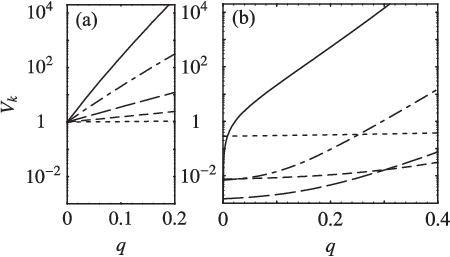

We finally note that if is fluctuating from run to run and hence becomes a random variable error correction is still possible. In this case we have to replace Eq. (24) by
| (31) | |||||
where is the probability density function of and denotes the BS error as a function of . The resulting system of linear equations Eq. (31) can be treated using the methods introduced above.
IV.1.2 Detector error
We now assume that only detector errors are present and each atom has a probability of failing to be detected. In this case is related to via
| (32) |
We can again solve this equation by methods similar to those used in Sec. IV.1.1 (though this time it is not a true inverse because the system is over-determined Foot2) to obtain
| (33) |
where non-integer values of are discarded. By combining Eqs. (22, 33) we obtain in terms of . For the remaining random error measured by we obtain the upper bound
| (34) |
Numerical calculations for confirm this exponential growth of with at . The results are shown in Fig. 8. This time, however, is typically much smaller than the analytic bound, e.g. for the cluster state, fitting gives . However, the exponential growth with implies a practical limit of for any contrary to the case of BS errors. This scaling can be improved by using the least squares method to handle the over-determined linear system of equations Eq. (32). We do not have an analytic bound analogous to Eq. (34) for the least squares method but numerical calculations for the cluster state and the worst case result in significantly lower values for than those obtained from Eq. (33). Most importantly as shown in Fig. 9 it appears that the scaling of becomes exponential in rather than similarly to the case of BS errors. This implies that an error of is acceptable for obtaining meaningful estimates of in a reasonable number of experimental runs.
In an actual experiment both BS and detector errors will be present and first correcting for the detector error using Eq. (33), then substituting the resulting for in Eq. (29) to correct for the BS error yields a combined analytical error bound of
| (35) |
According to our numerical results using the least squares method this bound can be improved requiring only for obtaining sufficiently small errors.
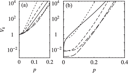

IV.2 With spatial resolution
If spatial resolution is available then , not just its average over all subsets of size , becomes accessible to measurement. This allows us to do some state characterizations which would otherwise be impossible and also introduces extra redundancy. As we will show below this does not affect the tolerance to BS errors but we will find that the detector error tolerance improves to . Imperfections in the spatial resolution, however, will lead to additional errors in determining .
IV.2.1 Beam splitter error
The variance of due to BS errors can be directly inferred from Eq. (27), where only the atoms in are counted. Using the same methods as in Sec. IV.1.1 we find an upper bound for (defined analogously to ) given by . The BS error tolerance (for fixed ) is thus independent of whether spatial resolution is available or not.
IV.2.2 Detector error
The situation is different for the detector error. Each antisymmetric pair contains two atoms only one of which needs to be detected to know that it was antisymmetric. Therefore the effective error probability becomes . The resulting formula is
| (36) |
where is the probability of measuring antisymmetric sites in subset . The variance bound is given by .
IV.2.3 Imperfect spatial resolution
There is a new type of error to consider as the spatial resolution itself will not in practice be perfect. If we let be the probability of finding at position a particle which is actually at position , then
| (37) |
where is the “set” (its elements are not necessarily distinct) of observed atom positions, and is the experimental probability of observing atoms exactly at these positions . The set denotes the antisymmetric sites and the probability of having antisymmetric sites at positions is , , and runs over all permutations of the atoms in . The -th element of and are written as and , respectively. The symmetry factor stands for the number of permutations which leave the ordered lists of atoms invariant (e.g., , ), and is needed because our summation runs over different ordered lists of the same set . This is an over-determined linear system, and just as in the case of detector error, we can either explicitly solve it by discarding some of the equations or apply the least squares method. As an explicit solution we can e.g. use
| (38) |
where we define . The sum runs over all ordered lists and is the matrix inverse of , that is .
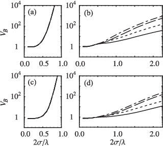
As before by performing numerical calculations using the least squares method we find much lower variances than with Eq. (38). An example is shown in Fig. 10 where we plot the variance of due to a Gaussian position error of the form
| (39) |
where is the standard deviation and is the wave length of the laser creating the optical lattice. The corresponding lattice spacing is . The results obtained from Eq. (38) shown in Fig. 10a, c require a resolution of whereas the least squares method shown in Fig. 10b, d yields reasonable variances for spatial resolutions up to . However, due to the exponentially large number of possibilities for the least squares calculation becomes intractable for large .
V Conclusion
We discussed the detection and characterization of multipartite entanglement in optical lattices with the quantum network introduced in Carolina2004 under different experimental conditions. We first described how the network can be implemented in ideal experimental conditions and showed that it allows to characterize a number of important classes of states like cluster-like states and macroscopic superposition states. We investigated the experimental realization of the network in an optical lattice and identified lack of spatial resolution, errors in the BS operation and imperfect atom detection as the main sources of error. We showed that even in the absence of spatial resolution entanglement can be detected. In cases where the entangled state is characterized by a few parameters only we found that these can often be determined from the measurement results. We also studied the influence of BS errors occurring with probability and detection errors with probability and concluded that with small numbers of experimental runs entanglement can be detected between atoms as long as and . Finally we showed that for obtaining purities of subsets rather than average purities with reasonable experimental effort a spatial resolution of is necessary.
The results obtained in this work show that unambiguous multipartite entanglement detection in optical lattices is possible with current technology. This has not yet been achieved experimentally BlochEnt. Furthermore it will even be possible to determine some of the characteristics of entangled states created in these experiments without the requirement of performing spatially resolved measurements. Our network is thus a viable alternative to detecting entanglement via witnesses or full quantum state tomography.
Acknowledgements.
This work was supported by EPSRC through the QIP IRC (www.qipirc.org) GR/S82176/01 and project EP/C51933/1, and by the EU network OLAQUI. C.M.A. thanks Artur Ekert for useful discussions and is supported by the Fundação para a Ciência e Tecnologia (Portugal).Appendix A The beam splitter operation
Since the BS only couples two lattice sites in rows I and II of each column (see Fig. 2) we consider a single such pair and omit the column superscript in this section. For , we obtain from the Heisenberg equations for the operators
| (40) |
Hence, applying for a time implements a perfect pairwise BS.
Initially the atom pair is in a state of the form , where is a single qubit state and hence has a spectral decomposition of the form , with , , and . Here , are linear superpositions of , with coefficients depending on . Therefore we can write
| (41) | |||||
which is a classical mixture of a symmetric state with probability and an antisymmetric state with probability . After the BS the resulting state is given by
| (42) | |||||
where , , are states with double occupancy in one row and an empty site in the other row while is a state with a singly occupied site in each row. Hence, after the BS we will find a doubly occupied site with probability while two singly occupied sites result with probability .
However, in practice it is impossible to completely turn off the interaction which may result in a symmetric state failing to bunch. We consider any symmetric state and because acts only on the row indices, not the internal states, and is symmetric between the two rows the probability of failure to bunch is given by
| (43) | |||||
The optimal choice for the BS time is for which . If the hopping term is not controlled perfectly accurately but fluctuates by around a mean we set and obtain Eq. (18).
References
- (1) D. Gottesman, Ph.D thesis (CalTech, Pasadena, 1997); A.M. Steane Phys. Rev. Lett. 77, 793 (1996); A.R. Calderbank, P.W. Shor, Phys. Rev. A 54, 1098 (1996).
- (2) R. Cleve, D. Gottesman, H.-K. Lo, Phys. Rev. Lett. 83, 648 (1999); D. Gottesman, Phys. Rev. A 61, 042311 (2000); A. Cabello, Phys. Rev. Lett. 89 100402 (2002).
- (3) R. Raussendorf, H.-J Briegel, Phys. Rev. Lett. 86, 910 (2001); R. Raussendorf, H.-J Briegel, Phys. Rev. Lett. 86, 5188 (2001).
- (4) P. Walther, K. J. Resch, T. Rudolph, E. Schenck, H. Weinfurter, V. Vedral, M. Aspelmeyer, A. Zeilinger, Nature 434, 169 (2005).
- (5) C. A. Sackett et al., Nature 404, 256 (2000); J. Chiaverini et al., Nature 432, 602 (2004).
- (6) O. Mandel et al., Nature 425, 937 (2003); D. Jaksch, H.-J. Briegel, J.I. Cirac, C.W. Gardiner, P. Zoller, Phys. Rev. Lett. 82, 1975 (1999).
- (7) S.E. Sklarz, I. Friedler, D.J. Tannor, Y.B. Band, C.J. Williams, Phys. Rev. A 66, 053620 (2002); S. Peil et al., Phys. Rev. A 67, 051603(R) (2003); W.K. Hensinger et al., Nature 412, 52 (2001).
- (8) Daniel F. V. James, Paul G. Kwiat, William J. Munro, Andrew G. White, Phys. Rev. A, 64, 052312 (2001).
- (9) C. Moura Alves and D. Jaksch, Phys. Rev. Lett. 93, 110501 (2004).
- (10) J. S. Bell, Physics 1 195, 1964; A. Aspect, P. Grangier, G. Roger, Phys. Rev. Lett. 49, 91 (1982).
- (11) B. Terhal, Phys. Lett. A 271, 319 (2000); M. Lewenstein, B. Kraus, J.I. Cirac, P. Horodecki, Phys. Rev. A 62, 052310 (2000).
- (12) M. Horodecki, P. Horodecki, R. Horodecki, Physics Letters A, 210, 377 (1996).
- (13) J. I. Cirac, M. Lewenstein, K. Molmer, and P. Zoller, Phys. Rev. A 57, 1208 (1998).
- (14) C. H. van der Wal et al., Science 290, 773 (2000); J. R. Friedman, V. Patel, W. Chen, S. K. Tolpygo, and J. E. Lukens, Nature 406, 43 (2000).
- (15) W. Dür, C. Simon, J.I. Cirac, Phys. Rev. Lett., 89, 210402 (2002).
- (16) R.F. Werner, Phys. Rev. A 40, 4277 (1989).
- (17) A.K. Ekert et al., Phys. Rev. Lett. 88, 217901 (2002); C. Moura Alves, D.K.L. Oi, P. Horodecki, A.K. Ekert, L.C. Kwek, Phys. Rev. A 68, 032306 (2003).
- (18) In the case of photon pairs this effect is known as Hong-Ou-Mandel interference and used in Bell state analysers: C. K. Hong, Z. Y. Ou, L. Mandel, Phys. Rev. Lett. 59, 2044 (1987); Klaus Mattle, Harald Weinfurter, Paul G. Kwiat, Anton Zeilinger, Phys. Rev. Lett. 76, 4656 (1996).
- (19) D. Jaksch, C. Bruder, J.I. Cirac, C.W. Gardiner, P. Zoller, Phys. Rev. Lett. 81, 3108 (1998); M. Greiner, O. Mandel, T. Esslinger, T.W. Haensch, I. Bloch, Nature 415, 39 (2002).
- (20) For a review of optical lattices, see D. Jaksch and P. Zoller, Annals of Physics 315, 52 (2005); D. Jaksch, Contemporary Physics 45, 367 (2004); I. Bloch, Physics World, 17, 25 (2004).
- (21) A. Widera et al., cond-mat/0310719.
- (22) If the resonant state is either or then there is also a suitable sequence of few pulses, which does not require phase locking, interleaved with suitable loss intervals: (i) a pulse that swaps and (ii) a pulse that takes to , followed by (iii) a second pulse.
- (23) In a perfect experiment an even number of atoms (two per antisymmetric pair) is always detected but in the presence of detector errord an odd number of atoms might arise.