Optimal squeezing and entanglement from noisy Gaussian operations

Squeezed states are a valuable resource for different fields of physics. They can increase the resolution of precision measurements, as exploited in gravitational wave detectors Caves, improve spectroscopic sensitivity spectroscopy, and enhance signal-to-noise ratios signal2noise, e.g., in optical communication. Moreover, squeezing acts as a basic building block for the generation of continuous variable entanglement EPR, which in turn is a cornerstone for quantum information purposes. Unfortunately, squeezing is an expensive resource as well: squeezed states are hard to create and the involved operations are subject to losses and noise inevitably restricting the attainable amount of squeezing. On the other hand passive operations, in quantum optical setups implemented by beam-splitters and phase shifters, can often be performed at low cost and they are—compared to the squeezers—relatively noiseless.

This work is devoted to the question, how can we exploit a given noisy squeezing device in an optimal way when supplemented by arbitrary noiseless passive operations. We derive the optimal strategy for single and repeated use of the squeezing device, calculate the achievable squeezing and relate it to the maximal attainable amount of entanglement. To this end we will use a black box model for the physical squeezing device. This will give us the possibility to derive optimality results which are equally applicable to a wide range of physical implementations.

The argumentation will make use of the covariance matrix formalism, which was mainly developed in the context of continuous variable states having a Gaussian Wigner distribution—so called Gaussian states HolevoBook. The latter naturally appear in quantum optical settings (the field of a light mode) as well as in atomic ensembles (collective spin degrees) and ion traps (vibrational modes). We restrict ourselves to the natural class of Gaussian operations, i.e., operations preserving the Gaussian character of a state CCR; Geza. This includes all time evolutions governed by operators quadratic in bosonic creation and annihilation operators. All the presented results hold for an arbitrary number of modes and although it might be reasonable to think in terms of Gaussian states, we do not have to restrict the input states to be Gaussian.

Preliminaries.—We will begin with introducing the notation and recalling some basic results HolevoBook; CCR; Geza; Jens. Consider a system of $N$ bosonic modes with respective canonical operators $(Q_{1},P_{1},\dots,Q_{N},P_{N})=\vec{R}$. These are related to the annihilation operators via $a_{j}=(Q_{j}+iP_{j})/\sqrt{2}$ and satisfy the canonical commutation relations $[R_{k},R_{l}]=i\sigma_{kl}\openone$ governed by the symplectic matrix $\sigma=\bigoplus_{i=1}^{N}\mbox{\footnotesize${\left(\begin{array}[]{cc}0&1\\ -1&0\end{array}\right)}$}\;.$ The displacement $\vec{d}$ in phase space and the covariance matrix (CM) $\gamma$ corresponding to a state $\rho$ are then given by

where $\{\cdot,\cdot\}_{+}$ denotes the anti-commutator.

While for coherent states $\gamma=\openone$, a state is called squeezed if its uncertainty in some direction in phase space is below the uncertainty of the coherent state, i.e., if $s(\gamma)\equiv\lambda_{\min}(\gamma)<1$, where $s(\gamma)$ is the squeezing of $\gamma$ measured by its smallest eigenvalue mukS. Note that by this definition, more squeezing means a smaller $s$. As the squeezing is independent of the displacement $\vec{d}$, we omit it for the remaining part of the paper.

Let us now focus on Gaussian operations. Unitary Gaussian operations are precisely those realizable by quadratic Hamiltonians, so that they naturally appear in many physical systems. In phase space they act as symplectic operations $S\in\mathrm{Sp}(2N)$ on the covariance matrix $\gamma\mapsto S^{T}\gamma S$. Symplectic operations preserve the canonical commutation relations and are thus given by the group $\mathrm{Sp}(2N)=\{S\in\mathbb{R}^{2N\times 2N}\,:\,S^{T}\sigma S=\sigma\}$. An important subgroup is given by the group of orthogonal symplectic transformations $\mathrm{K}(2N)=\mathrm{O}(2N)\cap\mathrm{Sp}(2N)$ mukS. Physically, these correspond to passive operations, which can, in quantum optical setups, be implemented by beam-splitters and phase shifters zeilinger. Obviously, passive transformations cannot change the squeezing, since elements from $\mathrm{K}(2N)$ preserve the spectrum and in particular the smallest eigenvalue of the CM.

We will now introduce the model we use to describe the squeezing device. In general, a noisy operation $\mathcal{E}$ can be regarded as a noiseless map on a larger system including the environment, which is discarded afterwards. If the overall time-evolution is governed by a quadratic Hamiltonian and the environment is in a Gaussian state (e.g., a thermal reservoir), it can be shown that these operations are exactly the ones which act as

with $X,Y\in\mathbb{R}^{2N\times 2N}$ CCR. Here, the equation on the right hand side ensures complete positivity, i.e., guarantees that the operation is physically reasonable. While the $X^{T}\gamma X$ part of $\mathcal{E}$ represents a joint rotation and distortion of the input $\gamma$, the $Y$ contribution is a noise term which may consist of quantum as well as classical noise. In the following, we will consider squeezing devices of the type in Eq. (1), as these are the ones which naturally appear in many experiments. We will, however, show at the end of the paper that the results even hold for arbitrary Gaussian operations (which may include measurements and conditional operations).

The question we are going to investigate is the following: given some noisy device $\mathcal{E}$ and the set of passive operations $\mathrm{K}(2N)$, how can we generate squeeezing as efficiently as possible from a given input state? Naturally, this general question can be asked in several specific ways. First of all, one might ask how much squeezing can be generated by a single application of the device given a certain initial state, as in Fig. 1a.

The much more interesting question, of course, relates to an iterative scenario, i.e., how can we generate squeezing as efficiently as possible by repeated application of $\mathcal{E}$ with passive operations $K_{i}$ inbetween (Fig. 1b)? In this scenario we may either allow for different $K_{i}$ or choose them identically as it is for instance the case in a ring cavity setup (Fig. 1c).

Single iteration.—In order to prepare for the more complicated scenarios, let us first have a look at the case of a single iteration (Fig. 1a), starting from a given input CM $\gamma$. This is the basic building block for all the iterative protocols. We now use a formal trick in order to facilitate the derivation: we split the CM into two parts (Fig. 2a),

where $s=s(\gamma)$ is the squeezing of $\gamma$. The first part can be regarded as a “coherent kernel” of $\gamma$. It may have sub-Heisenberg variance (if $s<1$) and it is invariant under passive operations. The second part is a “noise term” $N$ which ensures that $\gamma$ is a physical state. As $s$ is the smallest eigenvalue of $\gamma$, $N\geq 0$ has a null space.

Let us now see what happens if we rotate $\gamma=s\openone+N$ by some passive operation $K$ and then send it through $\mathcal{E}$: the coherent kernel is invariant under $K$, and thus

i.e., the action of the squeezing device on the “coherent kernel” plus the “noise” part which has been rotated and squeezed by $X$. Note that the first part no more depends on the choice of the passive operation; furthermore, as $N\geq 0$ and thus $X^{T}K^{T}NKX\geq 0$, the smallest eigenvalue of $\mathcal{E}(s\openone)$ gives a bound to the squeezing of the output. In the following, we show that this bound can be achieved. Therefore, let $s_{0}=s(\mathcal{E}(s\openone))=\lambda_{\min}[sX^{T}X+Y]$ be the squeezing obtained from the input $s\openone$ with corresponding eigenvector $|\phi\rangle$ footnote:bra-ket. On the one hand, $s^{\prime}\equiv s(\gamma^{\prime})\geq s_{0}$, and on the other hand,

Recall that by definition (2), $N$ has a null eigenvector which we denote by $|\nu\rangle$, $N|\nu\rangle=0$. By choosing $K$ such that $K(X|\phi\rangle)\propto|\nu\rangle$ (which can be always done with passive $K$, cf. mukS), the second term vanishes, and we indeed find that $s^{\prime}=s_{0}=s(\mathcal{E}(s\openone))$.

The proof is also illustrated in Fig. 2: Choosing $K$ appropriately ensures that the noise $N$ does not contribute in the most squeezed direction. Note that for a given $\mathcal{E}$ it is now straight forward to derive an optimal $K$ and by exploiting the results of zeilinger to decompose it into an array of beam-splitters and phase shifters.

For a single iteration of $\mathcal{E}$ this shows that the optimally achievable squeezing $s^{\prime}$ at the output is given by the squeezing obtained from the non-physical input $s\openone$:

It is highly interesting to note that, therefore, the optimal value of the final squeezing does only depend on the initial squeezing (and on the properties of $\mathcal{E}$), but on no other property of the initial state, irrespective of the number of modes considered. It can be easily checked that the respective function $f_{\mathcal{E}}$ in Eq. (3) is concave, monotonously increasing, and $f_{\mathcal{E}}(0)\geq 0$ (Fig. 3).

Multiple iterations.—The fact that the optimal output squeezing does only depend on the input squeezing immediately implies that in the case of multiple iterations the passive operations $K_{i}$ can be optimized successively in order to obtain the global optimum. This is a remarkable result, as in general problems of this kind require optimization over all parameters (i.e., over all $K_{i}$) simultaneously. Graphically, the squeezing in each iteration step moves along a zig-zag line between $f_{\mathcal{E}}(s)$ and the identity, as shown in Fig. 3. The optimal output squeezing $s_{\infty}$ (for number of iterations $\rightarrow\infty$) is determined by $f_{\mathcal{E}}(s_{\infty})=s_{\infty}$, $s_{\infty}\geq 0$. By inserting the definition (3) of $f_{\mathcal{E}}$ and solving for $s_{\infty}$ we obtain

The convergence of $s(\gamma_{i})$ to the optimal value is exponentially fast and bounded from above and below by the slope of $f_{\mathcal{E}}$ at $s_{\infty}$ and the slope from $(s_{\infty},f_{\mathcal{E}}(s_{\infty}))$ to the starting point $(s_{0},f_{\mathcal{E}}(s_{0}))$, respectively. Note that for $s(\gamma_{\mathrm{in}})<s_{\infty}$, however, $s(\gamma_{\mathrm{out}})>s(\gamma_{\mathrm{in}})$, so that squeezing is destroyed by applying the operation $\mathcal{E}$.

In realistic physical scenarios, it might be difficult to tune the passive operations independently and it is more likely that the same physical device will be passed again and again, e.g., in a ring cavity (cf. Fig. 1c), and thus only one fixed passive operation $K\equiv K_{i}\ \forall i$ can be implemented. In the following, we demonstrate that this is already sufficient to reach the optimal squeezing $s_{\infty}$. The proper $K$ is the one which preserves the squeezing at the optimality point, corresponding to a zig-zag line along the tangent of $f_{\mathcal{E}}$ at $s_{\infty}$. The convergence is thus still exponentially fast.

In order to see how this works, consider the non-physical output

obtained from the input $s_{\infty}\openone$. By the properties of $s_{\infty}$, it is clear that $\lambda_{\min}(\tilde{\gamma})=s_{\infty}$ with a corresponding normalized eigenvector $|\psi_{\infty}\rangle$. Now choose $K_{\infty}$ such that

This is exactly the $K$ which preserves the optimality point, as $|\psi_{\infty}\rangle$ is the null eigenvector of $\tilde{\gamma}-s_{\infty}\openone$. For any initial state $\gamma$ with $s(\gamma)>s_{\infty}$, choose the decomposition $\gamma_{0}=s_{\infty}\openone+P\;,$ where $P>0$ and $\lambda_{\min}(P)+s_{\infty}=s_{0}\equiv s(\gamma_{0})$. After one iteration $\gamma_{1}=\mathcal{E}(K_{\infty}^{T}\gamma_{0}K_{\infty})$, we have

As we will show in a moment, $\alpha<1$, and for the squeezing $s_{n}\equiv s(\gamma_{n})$ after $n$ iterations it holds by recursion that $s_{n}\leq s_{\infty}+\alpha^{n}\langle\psi_{\infty}|P|\psi_{\infty}\rangle$, which converges exponentially to $s_{\infty}$. From

it follows that

which is positive and strictly smaller than one as long as $\langle\psi_{\infty}|Y|\psi_{\infty}\rangle>0$, which is generically the case footnote:singularY.

Example.—Let us now consider an example which illustrates how the representation of the operation in Eq. (1) is related to the master equation $\dot{\rho}=i[\rho,\mathcal{H}]+\mathcal{L}[\rho]$ of a system. From it, one obtains a master equation for the evolution of the covariance matrix,

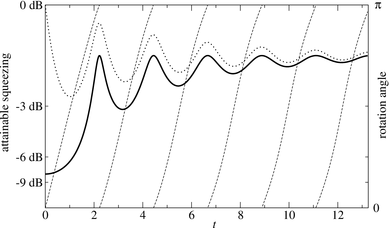
For the case of photon losses to a vacuum reservoir, $\mathcal{L}[\rho]=\nu(2a\rho a^{\dagger}-a^{\dagger}a\rho-\rho a^{\dagger}a)$, one obtains $A=2\sigma H-\nu\openone$ and $N=2\nu\openone$, where $H$ is the Hamiltonian matrix, i.e., $\mathcal{H}=(Q,P)H(Q,P)^{\dagger}$. By integration, one finds that applying (5) for a time $t$ leads to a map $\mathcal{E}_{t}:\gamma\mapsto X^{T}\gamma X+Y$ with $X=e^{-\nu t}\exp[-2H\sigma t]$ and

At this point, the results derived in the paper can be applied. Fig. 4 shows a one mode example with $\mathcal{H}=\frac{3}{4}a^{\dagger}a-\frac{1}{4}a^{\dagger}a^{\dagger}+\mathrm{h.c.}$ and the noise level $\nu=0.1$. Note that additional passive operations enhance the attainable squeezing although the noise $N$ is rotationally invariant.

Entanglement generation.—The optimality result on squeezing generation has direct implications for optimal entanglement generation. Indeed, it has been shown that the amount of entanglement which can be generated by passive operations starting from two squeezed Gaussian input states only depends on their squeezing irrespective of the number of modes WE; for two modes, e.g., this is done by sending the states onto a beam splitter after rotating them into orthogonal directions. Using this result, we can immediately determine how much entanglement we can generate from Gaussian inputs using a black box $\mathcal{E}$ supplemented by passive operations, namely $E_{\mathcal{N},\mathrm{opt}}=\log(s_{\text{opt}}^{-1})$, where $s_{\text{opt}}$ is the maximal squeezing generated by $\mathcal{E}$ and the entanglement is measured by the logarithmic negativity logneg. Moreover, by combining the results it is straightforward to explicitly derive the optimal entangling protocol for any given Gaussian device.

Acknowledgements.—We thank Klemens Hammerer and Jens Eisert for valuable discussions. This work has been supported by the EU (COVAQIAL), the DFG and the “Kompetenznetzwerk Quanteninformationsverarbeitung” der Bayerischen Staatsregierung.

Appendix.—In the following, we show that the results obtained for channels of the type (1) also hold for the most general type of Gaussian channels which may include measurements and postprocessing. Channels of this type appear, e.g., in the creation of spin squeezing using quantum nondemolition measurements with feedback mabuchi. The most general memoryless operation on $N$ modes can described by a $2N$ mode covariance matrix $\Gamma$ via the Jamiolkowski isomorphism Geza as

and $\tilde{\Gamma}$ is the partial transpose of $\Gamma$. Again, $s\equiv s(\gamma)$, $|\psi\rangle$ is the eigenvector corresponding to the smallest eigenvalue of $\mathcal{E}(s\openone)$, and we need to show that $K$ can be choosen such that $s(\mathcal{E}(s\openone))=s(\mathcal{E}(K\gamma K^{T}))$, i.e., that $\langle\psi|C(B+s\openone)^{-1}C^{T}|\psi\rangle=\langle\psi|C(B+K\gamma K^{T})^{-1}C^{T}|\psi\rangle$. This means that for $|\chi\rangle\equiv C^{T}|\psi\rangle$, $P\equiv(B+s\openone)>0$, and $N\equiv\gamma-s\openone\geq 0$ with a null eigenspace we have to find a $K$ such that

vanishes. Since $(*)$ has the same null eigenspace as $P^{-1/2}KNK^{T}P^{-1/2}$, the expression (6) can be indeed made zero by choosing $K$ such that $|\nu\rangle\propto K^{T}P^{-1}|\chi\rangle$ (where $N|\nu\rangle=0$). This proves that for any Gaussian operation the optimal output squeezing can be computed on $s\openone$, thus generalizing the results of the paper.

References

- (1) C.M. Caves, Phys. Rev. D 23, 1693 (1981).
- (2) E.S. Polzik, J. Carri, H.J. Kimble, Phys. Rev. Lett. 68, 3020 (1992); N.Ph. Georgiades et al., Phys. Rev. Lett. 75, 3426 (1995).
- (3) M. Xiao, L.A. Wu, H.J. Kimble, Phys. Rev. Lett. 59, 278 (1987); P. Grangier et al., Phys. Rev. Lett. 59, 2153 (1987).
- (4) Z.Y. Ou et al., Phys. Rev. Lett. 68, 3663 (1992); C. Silberhorn et al., Phys. Rev. Lett. 86, 4267 (2001); W. P. Bowen et al., Phys. Rev. Lett. 90, 043601 (2003).
- (5) A.S. Holevo, Probabilistic and statistical aspects of quantum theory, North-Holland Publishing Company, 1982.
- (6) B. Demoen, P. Vanheuverzwijn, A. Verbeure, Lett. Math. Phys. 2, 161 (1977).
- (7) G. Giedke, J.I. Cirac, Phys. Rev. A 66, 032316 (2002); J. Fiurasek, Phys. Rev. Lett. 89, 137904 (2002).
- (8) J. Eisert, M.B. Plenio, Int. J. Quant. Inf. 1, 479 (2003).
- (9) R. Simon, N. Mukunda, B. Dutta, Phys. Rev. A 49, 1567 (1994).
- (10) M. Reck et al., Phys. Rev. Lett. 73, 58 (1994).
- (11) Note that we use bra-kets to denote ordinary vectors. This is not a quantum state.
- (12) The case of singular requires a lengthy discussion which, however, does not give any new insight, therefore, it has been omitted.
- (13) M.M. Wolf, J. Eisert, M.B. Plenio, Phys. Rev. Lett. 90, 047904 (2003).
- (14) G. Vidal, R.F. Werner, Phys. Rev. A 65, 032314 (2002).
- (15) J.M. Geremia, J.K. Stockton, and H. Mabuchi, Science 304, 270 (2004).