Quantum computation via translation-invariant operations on a chain of qubits

The key to the construction of a universal set of gates for the described automaton is displayed in Fig. 1. The $N+1$-fold repetition of the elementary transition function constitutes half a clock cycle of the automaton. Within this period each local Pauli observable goes through the phases of expansion, transmission, and contraction to the mirror image of the initial position. During expansion and contraction, the propagated observable is susceptible to a global $Y$-pulse

Namely, it picks up a sign factor under conjugation. Contrarily, during the phase of transmission where the observables behave as left- or right-movers SW a $Y$-pulse has no effect. The duration of expansion, transmission and contraction phase depend on the initial position of the local Pauli observable. Therefore, each local Pauli observable shows a characteristic response to sequences of $Y$-pulses within the half-cycle. In this way, temporal control can be translated into spatial control. In the construction described below, suitably tailored sign-flips of Pauli observables are used to reverse rotation angles. Depending on whether a rotation angle is reversed or not, two matching rotations will either cancel or amplify each others effect.

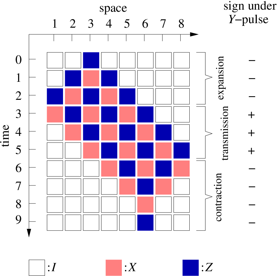
The degree of spatial control obtained suffices to simulate a quantum logic network. One constraint arises: every operation applied to the qubit chain is reflection-symmetric. Therefore, qubit $i$ cannot be addressed separately from its mirror image at location $\overline{i}:=N+1-i$. To cope with this constraint, the same network is simulated twice on the chain, once on the left side and once—as mirror image—on the right. This doubles the required length of the chain and also influences the readout process, as will be discussed in Section II $b$.

To probe the available spatial control, consider the sequence

where $\textbf{c}=(c_{0},..,c_{N})^{T}$ is a binary vector. To analyze the effect of this sequence, the Pauli operators $Y^{c_{i}}$ are propagated backwards in time until they reach the $U_{Z}$-gates. There they accumulate to $\overline{Y}$,

Then,

where we have used that $R\overline{Y}R=\overline{Y}$, and

In this way, temporal control has been converted into spatial control, provided that—for suitable choices of ${\bf{c}}$—the binary variables $s_{i}({\bf{c}})$ do indeed vary with $i$.

The $s_{i}$ are easily computed in the stabilizer formalism Go-DeMoor. Following DeMoor, we write Pauli operators $A$ in the form $i^{\delta}(-1)^{\epsilon}\tau_{\textbf{a}}$, where $\textbf{a}=\left(\begin{array}[]{c}\textbf{z}\\ \textbf{x}\end{array}\right)$ is a 2$N$-component binary vector, $\textbf{z}=(v_{1},..,v_{N})^{T}$, $\textbf{x}=(w_{1},..,w_{N})^{T}$; $\delta,\epsilon\in\mathbb{Z}_{2}$, and $\tau_{\bf{a}}=\bigotimes_{i=1}^{N}Z_{i}^{v_{i}}X_{i}^{w_{i}}$. The evolution of $A$ under conjugation by our Clifford unitary $T$, $A\longrightarrow T(A)=TAT^{\dagger}$, may then be followed in terms of $\delta$, $\epsilon$ and a. The scalars $\delta$ and $\epsilon$ have no influence on the sign factor $(-1)^{s_{i}}$ (8), and we need to consider the update of a only, $\textbf{a}(t)\longrightarrow\textbf{a}(t+1)=C\textbf{a}(t)$. Therein, $C$ is a $2N\times 2N$ binary symplectic matrix which takes the form

$\Gamma$ is the adjacency matrix of the interaction graph (the line graph). Further, denote by $F$ the $2N\times 2N$-matrix $F=\left(\begin{array}[]{cc}0&I\\ I&0\end{array}\right)$ and observe that $FC^{-1}=CF$. Now, the vector $\textbf{s}=(s_{1},..,s_{N})^{T}$ carrying the information about the sign flips under conjugation by $\overline{Y}$ is related to the vector c describing the temporal sequence of $Y$-pulses, via $\textbf{s}=M_{Z}{\bf{c}}$. The matrix $M_{Z}$ encodes how temporal control is converted to spatial control. Its elements are given by

The binary quantities $M_{Z}(i,t)$ can be defined for all $t$ ($i=1..N$). But the matrix $M_{Z}$ is the collection of $M_{Z}(i,t)$ only within the half-cycle $0\leq t\leq N$.

For the interval $t\in[-1,N]$ (including $[0,N]$) the $M_{Z}(i,t)$ take the values

Therein, the addition is modulo 2 and the step function $\theta$ is equal to one for all non-negative arguments, and zero otherwise.

To prove (11) one may—in addition to $M_{Z}$—define a matrix $M_{X}$ that encodes the sign factor acquired by the $t$-steps-backward-propagated observable $X_{i}$ under conjugation with $\overline{Y}$, $M_{X}(i,t):=\textbf{a}_{X_{i}}^{T}C^{t}\textbf{a}_{Y}$. Then, because of $TX_{i}T^{-1}=Z_{i}$ and $TZ_{i}T^{-1}=X_{i}\bigotimes_{j|\,\Gamma_{ij}=1}Z_{j}$, the $M_{Z}(i,t)$ and $M_{X}(i,t)$ obey the recursion relations

The solution of the recursion relation for $M_{Z}(i,t)$ is unique once the boundary conditions on two consecutive time slices are specified. In the discussed case, the boundary conditions are $M_{Z}(i,-1)=M_{Z}(i,0)=1$, for all $i=1..N$. The expression on the r.h.s of (11) obeys the recursion relation (12) in the interval $0\leq t\leq N-1$ and the boundary conditions, and is thus the correct expression for $M_{Z}$.

To perform a $z$-rotation on qubit $i$, one may apply a $Y$-pulse at times $i-1$ and $i$. For $c_{t}=\delta(t,i-1)+\delta(t,i)$, with (11), one obtains $s_{j}=\delta(j,i)+\delta(j,N+1-i)$. Therefore, the pulse for a $z$-rotation of qubit $i$ is

with $\overline{i}=N+1-i$ the mirror site of $i$. In this way, two out of $N$ $z$-rotations can be selected. A further discrimination between two sites $i$ and $\overline{i}$ is not possible because of the reflection symmetry of every sequence $U({\bf{c}},\alpha)=RU({\bf{c}},\alpha)R^{-1}$. As a result of this symmetry, each quantum algorithm is run on the qubit chain in two copies, one being the mirror image of the other. This accounts for a factor of two in spatial overhead.

From (13) the remaining universal gates can be deduced easily. Relation (13) is conjugated by $T^{-1}$. Using $T^{-1}Z_{i}T=X_{i}$, one finds

Conjugating relation (14) again by $T^{-1}$ and noting that $T^{-1}X_{i}T=Z_{i}\bigotimes_{j|\,\Gamma_{ij}=1}X_{j}=:K_{i}$ one obtains

Now, the length of the chain is doubled a second time. Specifically, the logical qubits in state $|\psi\rangle$ are interlaced by ancilla qubits which remain in the state $|0\rangle$ throughout the computation,

At this point it is suitable to introduce a logical coordinate $[j]$ that is related to the physical location within the qubit chain via $[j]=2j-1$, for $1\leq j\leq n$, such that e.g. $|\psi^{\prime}\rangle=|\psi\rangle_{[1],[2],..,[n]}\otimes|0..0\rangle_{2,4,..,2n-2}$. Then, the action of the $K_{2j}$ gate is equivalent to a two-qubit next-neighbor entangling gate,

The gates (13), (14) and (15) form a gate set that can be easily converted into the standard universal set Boy.

As an example for global readout I consider a measurement of the $z$-component of the total spin, i.e., of the observable

This is a model for readout e.g. of atomic qubits via resonance fluorescence spectroscopy, if the atoms are well within the Lamb-Dicke limit (their separation and fluctuation of position are much smaller than the optical wave length). In this case the underlying physics prohibits the extraction of local information. The readout method described below equally works for a scenario where a local readout could in principle be performed but is not pursued due to technological limitations. For specification of such a measurement model, see remark 3 in Section III.

With the capability to perform arbitrary unitary evolution on a quantum register the total spin observable $S_{Z}$ acting on that register may be conjugated into any desired observable, and the standard network readout of the individual $Z_{i}$ should be feasible. However, for the setting described here the readout procedure is, in the case of probabilistic algorithms, slightly complicated by the fact that two copies of the algorithm are run simultaneously and the readout measurement couples them.

For the readout each of the two circuits on the chain requires one additional logical qubit that is in the state $|0\rangle$ until the readout starts. The location of this qubit within the logical quantum register is denoted as $[0]$ which shall correspond to the physical position $2n+1$ in the qubit chain (see Fig. 2a). The readout consists of three steps. First, $S_{Z}$ is measured and the outcome $m$ is recorded. Second, for all logical qubits $j=1..n$ the following procedure is performed: 2.1) Apply CNOT gates $\Lambda(X)_{[j],[0]}\otimes\Lambda(X)_{\overline{[j]},\overline{[0]}}$ ([0], $\overline{[0]}$ are the target qubits). 2.2) Measure the observable $S_{Z}$ and record the outcome $m(j)$. 2.3) Apply the CNOT gates $\Lambda(X)_{[j],[0]}\otimes\Lambda(X)_{\overline{[j]},\overline{[0]}}$ again. Third, denote by $J=\{j_{1},..,j_{|J|}\}$ those $j\leq n$ for which $m-m(j)=2$. If $|J|<2$ the readout is finished. Otherwise, for all $k=2..|J|$ perform the following procedure: 3.1) Apply the Toffoli-gates $\Lambda_{2}(X)_{[j_{1}],[j_{k}];[0]}\otimes\Lambda_{2}(X)_{\overline{[j_{1}]},\overline{[j_{k}]};\overline{[0]}}$ ([0], $\overline{[0]}$ are the target qubits), 3.2) Measure $S_{Z}$ and record the measurement outcome $m(j_{1},j_{k})$. 3.3) Apply the Toffoli-gates $\Lambda_{2}(X)_{[j_{1}],[j_{k}];[0]}\otimes\Lambda_{2}(X)_{\overline{[j_{1}]},\overline{[j_{k}]};\overline{[0]}}$ again.

The conditional phase- and Toffoli gates are their own inverse such that the above protocol amounts to a sequence of measurements where the first one is of $S_{Z}$ and the following ones are of conjugated observables. These observables mutually commute because they are all diagonal in the computational basis, and the final state is a simultaneous eigenstate of them. The observables measured in step 2 are $Z_{[0]}Z_{[j]}+Z_{\overline{[0]}}Z_{\overline{[j]}}+\sum_{i\neq[0],\overline{[0]}}Z_{i}$. Since the qubits at locations $[0]$ and $\overline{[0]}$ are individually in the state $|0\rangle$, and the observable $S_{Z}=\sum_{i}Z_{i}$ already has been measured in step 1, step 2 effectively acts as the measurement of the observables $Z_{[j]}+Z_{\overline{[j]}}$.

Similarly, step 3 amounts to the measurement of the observables $|11\rangle_{[j_{1}],[j_{k}]}\langle 11|+|11\rangle_{\overline{[j_{1}]},\overline{[j_{k}]}}\langle 11|$, $\forall k$. This measurement assigns a sharp value to $r_{[j_{1}]}r_{[j_{k}]}+\overline{r}_{[j_{1}]}\overline{r}_{[j_{k}]}$. Its purpose is, in combination with the information gathered in step 2, to discriminate between the two cases $\{r_{[j_{1}]}=r_{[j_{k}]},\overline{r}_{[j_{1}]}=\overline{r}_{[j_{k}]}\}$ and $\{r_{[j_{1}]}\neq r_{[j_{k}]},\overline{r}_{[j_{1}]}\neq\overline{r}_{[j_{k}]}\}$, for each $k$.

The state of the two quantum registers after the measurement, leaving out all the ancillas in the state $|0\rangle$, may be written as a superposition $\sum_{\alpha}c_{\alpha}|\textbf{r}^{(\alpha)}\rangle|\overline{\textbf{r}}^{(\alpha)}\rangle$ of computational basis states $|\textbf{r}^{(\alpha)}\rangle|\overline{\textbf{r}}^{(\alpha)}\rangle$, where $\textbf{r}=(r_{[1]},..,r_{[n]})^{T}$, $\overline{\textbf{r}}=(r_{\overline{[1]}},..,r_{\overline{[n]}})^{T}$. The measurements then impose constraints upon which basis states are admissible, i.e., occur with nonzero coefficients $c_{\alpha}$. The constraints imposed by the measurements in step 2 read

for all $j=1..N$. The constraints that arise from the measurements in step 3 are

for $[j_{1}],[j_{k}]\in J$, $k=2..|J|$. The system (19, 20) of linear equations has a unique solution if $J=\emptyset$ and two solutions otherwise. In the latter case, the two solutions $\textbf{r}^{(1)}$ and $\textbf{r}^{(2)}$ correspond to two states $|\textbf{r}^{(1)}\rangle|\textbf{r}^{(2)}\rangle$ and $|\textbf{r}^{(2)}\rangle|\textbf{r}^{(1)}\rangle$, and the state of the quantum register after readout is their reflection-symmetric linear combination. The solutions $\textbf{r}^{(1)}$ and $\textbf{r}^{(2)}$ are, modulo interchange, uniquely specified by the measurement outcomes $m$, $\{m(j)\}$ and $\{m(j_{1},j_{k})\}$. For a probabilistic algorithm, the automaton produces two potential solutions in each run.

For the described method of universal computation via translation-invariant interaction it is relevant that the elementary transition function $T$ repeated a sufficient number of times reduces to the identity operation. Such an elementary ‘clock cycle’ takes $2(N+1)$ time steps where $N$ is the length of the chain. But as described so far, one still ends up with a set of local and next-neighbor gates and thus pays the price of next-neighbor slowdown twice. This is not necessary. Before the resources are counted, a long-distance entangling gate is described. As compared to a logically equivalent composition of next-neighbor and local gates, it cuts the required operational resources by a factor of order $n$.

The natural gate set for the described scheme of quantum computation does not only contain local and next-neighbor gates, but all gates of the form

As before, the logical position $[l]$ corresponds to the physical location $2l-1$ in the chain. The sequence for implementing $U_{X}(\alpha,L_{1},L_{2})$ is

with $t_{1}=L_{2}-L_{1}$, $t_{2}=L_{1}+L_{2}-2$ and $t_{3}=N-2L_{1}+2$. Now note that, with $|-\rangle:=-X|-\rangle$,

Thus, a long-distance $x$-controlled spin-flip can be implemented with 4 elementary gates (22). These four operations can be grouped into two pairs, with constant value of $L_{2}$ in each pair. Either pair of operations can be implemented in one clock cycle because the $Y$-pulse sequences of the two operations coincide. An $x$-controlled spin-flip thus takes two clock cycles irrespective of the distance between control and target qubit.

Now counting the resources, a quantum computation on $n$ qubits in the described scheme requires a qubit chain of length $N=4n+2$. Each clock cycle takes $8n+6$ elementary time steps (applications of $T$), and each of the universal gates $\exp\left(i\alpha/2\,Z_{l}\right)$, $\exp\left(i\alpha/2\,X_{l}\right)$ and $e^{i\pi|--\rangle_{l_{1},l_{2}}\langle--|}$ takes at most two clock cycles. As compared to the network model, there arises a constant overhead of $4$ in the spatial and a linear overhead of $16n$ in temporal resources.