Security of two quantum cryptography protocols using the same four qubit states

Let us start by summarizing the results presented in [11, 12], where a computable lower bound on the secret key rate for a general class of QKD protocols using one–way classical post–processing has been derived. We use the entanglement–based description of the protocol. Alice prepares $n$ qubit–pairs at random in one of the states defined in Eq. (4) and sends the second qubit of each pair to Bob. Eve might now apply the most general attack on all the qubits sent to Bob. Bob applies at random one of the operators defined in Eq. (5) on the qubits he received. After that Alice and Bob symmetrize their qubit pairs by applying a random permutation on them. On the other hand, Alice and Bob randomly choose for each qubit pair to apply the bit flip operation ($\sigma_{x}\otimes\sigma_{x}$). Both of those transformations commute with their measurement in the $z$–basis. It has been shown in [11] that after randomly applying these transformation the form of the state describing Alice’s and Bob’s system is Bell-diagonal, independently of the protocol. Its eigenbasis is given by $\{\mbox{$|\Phi^{+}\rangle$}^{\otimes n_{1}}\mbox{$|\Phi^{-}\rangle$}^{\otimes n_{2}}\mbox{$|\Psi^{+}\rangle$}^{\otimes n_{3}}\mbox{$|\Psi^{-}\rangle$}^{\otimes n_{4}}\}$, where $n_{1}+n_{2}+n_{3}+n_{4}=n$ and the states $\mbox{$|\Phi^{\pm}\rangle$},\mbox{$|\Psi^{\pm}\rangle$}$ denote the Bellbasis. Apart from that the state is symmetric with respect to exchanging the different qubit–pairs. The only free parameters are the eigenvalues of the density operator. Those depend on the distribution of the quantum information, i.e. on the QKD protocol. It is important to note that when assuming that Eve has a purification of this state, i.e $\rho_{ABE}=\mbox{$|\Psi\rangle$}_{ABE}\mbox{$\langle\Psi|$}$, for some state $\mbox{$|\Psi\rangle$}_{ABE}$, then her power is never underestimated. It has then be shown in [11, 12] that a lower bound on the secret key rate can then be determined considering only two–qubit density operators. In particular, for a given QBER, $Q$, a lower bound on the secret key rate (assuming that Alice and Bob apply optimal error correction and privacy amplification) is given by

with

Here, $S$ ($H$) denotes the von Neumann (Shannon) entropy respectively. It is important to take some space to describe these objects in detail.

• •

  The first apparent thing is that Alice does something to her bit string $A$ which transforms them to $A^{\prime}$. This is called preprocessing. It is a classical operation, known only to her (just note that in the original formula, Eq. (2) in [11], there appears also the possibility, noted $V$ there, that Alice discloses something of her preprocessing publicly: neglecting this possibility here, we can nevertheless obtain a lower bound). We consider here that Alice applies this preprocessing to each bit value independently. Thus, she can only flip her bit values with a certain probability. Note that this transformation reduces the information Bob has about Alice’s bit string, but it turns out that it penalizes Eve more than Bob, which implies that this preprocessing increases the secret key rate. Obviously, Alice will choose the preprocessing which maximizes the rate, whence the ”supremum” in (9).

• •

  The set $\Gamma_{Q}$ can be assumed to contain only two–qubit Bell–diagonal density operators which are compatible with the measured QBER $Q$. In order to be more precise we have to introduce the following notation. We denote by $\rho_{0}=\mathrm{tr}_{E}[{\cal E}(\mbox{$|\Phi^{+}\rangle$}_{AB}\mbox{$\langle\Phi^{+}|$}\otimes\mbox{$|0\rangle$}_{E}\mbox{$\langle 0|$})]$, where ${\cal E}$ denotes a general map applied by Eve (we do not impose that this map is unitary, since we are going to consider in the following the state shared by Alice and Bob after sifting). Let us denote now by $A_{j}$, $B_{j}$ the decoding/encoding operators defined by the considered protocol. For the SARG04 protocol, these are the operators defined in Eq. (3) and Eq. (5), respectively. The state describing Alice’s and Bob’s qubit pairs after sifting can be considered to be

  $\displaystyle\rho_{1}={\cal D}_{1}(\rho_{0})=C\,\sum_{j}A_{j}\otimes B_{j}\,\rho_{0}\,A_{j}^{\dagger}\otimes B_{j}^{\dagger}$

  (11)

  where $C$ is a normalization constant which may depend on $\rho_{0}$ (recall that e.g. in SARG04, the length of the sifted key varies with the amount of errors). Recall that this state is measured by Alice and Bob in the $z$–basis. Using this notation we can now define the set $\Gamma_{Q}$. It contains any state of the form

  $\displaystyle\rho_{2}$

  $\displaystyle=$

  $\displaystyle\lambda_{1}P_{\Phi^{+}}+\lambda_{2}P_{\Phi^{-}}+\lambda_{3}P_{\Psi^{+}}+\lambda_{4}P_{\Psi^{-}}$

  (12)

  with

  $\displaystyle\begin{array}[]{lcl}\lambda_{1}&=&\mbox{$\langle\Phi^{+}|\rho_{1}|\Phi^{+}\rangle$}\\ \lambda_{2}&=&\mbox{$\langle\Phi^{-}|\rho_{1}|\Phi^{-}\rangle$}\\ \lambda_{3}&=&\mbox{$\langle\Psi^{+}|\rho_{1}|\Psi^{+}\rangle$}\\ \lambda_{4}&=&\mbox{$\langle\Psi^{-}|\rho_{1}|\Psi^{-}\rangle$}\end{array}\,.$

  Those coefficients have to fulfill the normalization condition and the fact that the state $\rho_{2}$ has to be compatible with the estimated error, $Q$. Since the state is measured in the computational basis this implies

  $\displaystyle\begin{array}[]{lcl}\lambda_{1}+\lambda_{2}&=&1-Q\,,\\ \lambda_{3}+\lambda_{4}&=&Q\,.\end{array}$

  The considered protocol, i.e. the map ${\cal D}_{1}$ confines the $\lambda$’s further. Let us denote now by $\sigma_{AB}\in\Gamma_{Q}$ the state describing Alice’s and Bob’s qubit. Eve is supposed to hold a purification of this state, i.e $\sigma_{ABE}$ is pure. Obviously, one must suppose that Eve has made the best attack, whence the ”infimum” in Eq (9).

• •

  The density matrix $\sigma_{A^{\prime}E}$ is the state of the joint system of Alice and Eve, after Alice has performed the preprocessing.

• •

  As for $R(\sigma_{A^{\prime}BE})$: if one would replace the von Neumann entropy $S$ by the Shannon entropy $H$, this boils down to $H(A^{\prime}|E)-H(A^{\prime}|B)=I(A^{\prime}:B)-I(A^{\prime}:E)$, giving the usual Csiszár-Körner bound [19], see Eq. (41) below. What appears in Eq. (9) is thus its ”quantum analog”, given that Eve is allowed to keep her systems quantum.

Now, we have announced that one can compute a lower bound on the secret key rate considering only two–qubit Bell–diagonal states. Precisely, this is true if Alice’s preprocessing is bit-wise. In general, it holds that: if Alice’s preprocessing is applied to strings of $n$ bits, then one can restrict to Eve’s collective attacks on $n$ pairs. If we note $r_{n}$ the corresponding bound for the secret key rate $r$, one has $r\geq r_{n}\geq r_{1}$; it is an open problem, whether strict inequalities hold.

In summary, we are going to compute the lower bound on the secret key rate if Alice applies a bit-wise preprocessing, i.e. Eq. (9). The quantity $R(\sigma_{A^{\prime}BE})$ is given in Appendix A as an explicit function of the $\lambda_{i}$. This expression is independent of the protocol: as mentioned above, only the constraints on the $\lambda_{i}$, that is the set $\Gamma_{Q}$, depend on the protocol. Possible improvements on the bound may come from more-than-one-bit preprocessing, and/or from revealing a part of the preprocessing publicly.

The SARG04 protocol uses all the four sifting sets ${\cal S}_{\sigma\omega}$ (a different bound is found if one considers a modified protocol which uses only two sets, see Appendix B). One finds after some algebra

The following relations then hold:

Supposing that we leave $\lambda_{2}=x$ free, we obtain $\lambda_{1}=1-Q-x$ from (• ‣ III.2.1), $\lambda_{3}=x-\frac{Q}{2}$ and $\lambda_{4}=\frac{3Q}{2}-x$ from (26); the positivity of $\lambda_{3}$ and (27) restrain $x$ to lie in the range $[Q/2,Q]$. We optimize $r_{1}$ and find it positive provided $Q\leq 10.95\%$. If we’d have neglected the pre-processing, we’d have found $Q\leq 9.68\%$, the same value obtained by Tamaki and Lo [9, 20].

We start by describing the unitary ${\mathcal{U}}$ which we have found. It is defined by its action on the $z$–basis of the qubit flying from Alice to Bob and on a reference state used by Eve as:

with $\sigma=\pm$ and $\mbox{$|\psi_{\sigma}(D)\rangle$}=\sqrt{1-D/F}\mbox{$|0\rangle$}+\sigma\sqrt{D/F}\mbox{$|1\rangle$}$. Here, $D\in\left[0,\frac{1}{2}\right]$ is the only free parameter of the transformation. Note that Eve’s system is only 3-dimensional; we used a two-qubit notation for convenience. In fact, with this notation, the action of the unitary in the $x$–basis is similar to its action on the $z$–basis, but the roles of $E_{1}$ and $E_{2}$ are reversed: writing with $\omega=\pm$, one has

We suppose in the following that Alice publicly announces the set $\{\mbox{$|+z\rangle$},\mbox{$|+x\rangle$}\}$ (i.e. Alice actually sends one of these two states), and that Bob accepts the bit. It has been verified that thanks to the symmetries of the attack, all the following still holds if Alice sends another state and/or announces another set.

Bob’s states: Suppose for definiteness that Alice sends the state $|+z\rangle$. If we trace over Eve’s system, we get Bob’s state :

Thus the effective channel induced on Alice-Bob by Eve’s attack is a depolarizing channel (1) with disturbance $D$. If Bob measures his qubit in the $z$ basis, then he will accept the (wrong) conclusive result $|-z\rangle$ with probability $p_{acc}^{\,z}=D$. If Bob now measures his qubit in the $x$ basis, he will accept the (right) conclusive result $|-x\rangle$ with probability $p_{acc}^{\,x}=\mbox{$\langle-x|$}\rho_{B}\mbox{$|-x\rangle$}=1/2$. The quantum bit error rate after sifting (QBER) is therefore:

Note that, contrary to the case of BB84, $Q\neq D$; for small values of $D$ we have actually $Q\simeq 2D$. We shall come back to this point in the comparison with BB84, paragraph III.4 below.

Eve’s states: After sifting, Eve has to distinguish between four states, corresponding to the two possible states announced by Alice and the two cases in which Bob accepts the item. We write these states as $|\widetilde{\psi}_{E}^{ab}\rangle$, where $a$ (resp. $b$) $\in\{0,1\}$ denote Alice’s (resp. Bob’s) classical bit:

with $\mbox{$|\Psi^{-}\rangle$}=\frac{1}{\sqrt{2}}\,(\mbox{$|01\rangle$}-\mbox{$|10\rangle$})$. Note that these states are not normalized, but the square of their norms correspond to the probabilities with which they appear. Eve should now distinguish at best between these four states.

We suppose that Eve uses the Helstrom strategy to guess Alice’s bit [21]. This strategy, which may not be the optimal one for the present problem, consists in measuring the observable

where

Some analytical results, which provide also a different perspective on Helstrom’s strategy, are given in Appendix C. Here we just sketch the calculation that can also be implemented numerically from the beginning. There are three possible outcomes $e$ for Eve’s variable $E$. The probability of each outcome is

with $\rho_{E}=\frac{1}{2}\rho_{E}^{A=0}+\frac{1}{2}\rho_{E}^{A=1}$. The information Eve gets on Alice’s bit is

where $h$ is binary entropy and where

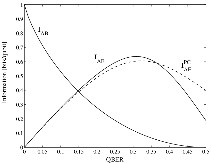
with $p_{E=e|A=0}=\mbox{$\langle m_{e}|$}\rho_{E}^{A=0}\mbox{$|m_{e}\rangle$}$. This information is plotted together with Bob’s information $I(A:B)=1-h(Q)$ as a function of the QBER, Eq. (31), in Fig. 1. The curve of $I(A:E)$ for the attack using the phase-covariant cloning machine, taken from Ref. [8], is included for comparison. Our attack is slightly more efficient in the interesting region.

Actually, if Eve performs the measurement of $M_{A}$, she has a good guess on Alice’s bit but a very poor information on Bob’s bit (the only thing she knows is that Bob’s bit is equal to Alice’s with probability $1-D$). Similarly, with reversed roles, if Eve would measure $M_{B}=\rho_{E}^{B=0}-\rho_{E}^{B=1}$: numerically, the $I(B:E)$ so found is equal to $I(A:E)$ found when measuring $M_{A}$; but now, Eve has poor information on Alice’s bit. For BB84 and the six-state protocols, measurements have been explicitly found which attain the optimal value for both Alice’s and Bob’s bits. We did not find such a measurement here. However, this is not important: before starting error correction and privacy amplification, Alice and Bob must choose whether to perform the direct or the reverse reconciliation; thus Eve can simply choose the suitable measurement.

An upper bound on the attainable secret key rate using one-way communication and single-bit preprocessing is given by the Csiszar-Körner bound [19] which reads

where $A^{\prime}$ is the result of a local processing of Alice’s variables. The need for this maximization went unnoticed in the field of QKD until very recently [11], but is indeed present in the original paper. Here, we consider the case when the process $A\rightarrow A^{\prime}$ consists in Alice’s flipping her bit with some probability $q$. Bob’s information is now

where

As for Eve’s information, it can be calculated with Eq. (39) upon changing $p_{A=0|E=e}$ to

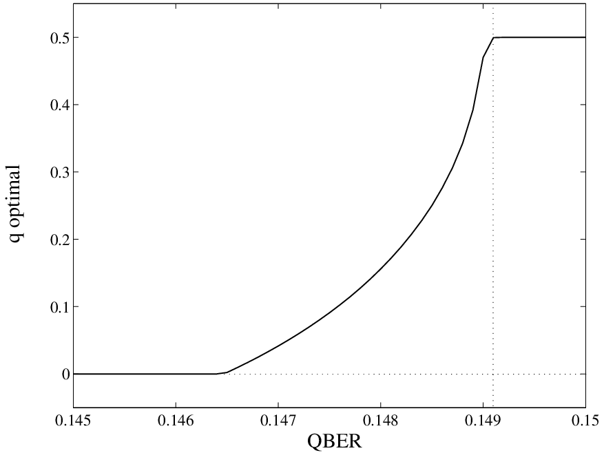
Fig. 2 displays the upper bound on the secret key rate, Eq. (41), with and without Alice’s bit flipping (upper graph) and the corresponding optimal value of $q$ (lower graph) as a function of the QBER. We can see that this preprocessing allows Alice and Bob to slightly increase the bound on the QBER where the achievable secret key rate becomes zero. In the case where Alice performs bit-wise preprocessing as we consider here, this bound is 14.9%. Alice will do this preprocessing only for a QBER close to the bound of 14.9%, with $q$ increasing as the QBER increases. At the bound, $q=0.5$: Alice flips half of her bits, so that both Bob’s and Eve’s information on her bits is completely randomized. After this optimal preprocessing, Fig. 1 would look as follows: both $I(A:B)$ and $I(A:E)$ stay the same up to $Q\approx 14.6\%$; then suddenly both drop rapidly to zero, with their difference given in the upper graph of Fig. 2.

No preprocessing was taken into account in Ref. [8] for the attack using the phase-covariant cloner. When one includes bit-wise preprocessing, the bound for that attack moves from 15.03% to 15.12%. Consequently, the attack presented here is still more efficient from Eve’s standpoint.

When $n$ photons arrive, the probability of not having any click is independent of the basis chosen by Bob and is given by

The corresponding zero-click rate is $C_{0}=\sum_{n\geq 0}p_{B}(n)p_{0}(n)=(1-p_{d})^{2}\,p(0|\mu t\eta)$ i.e. there are no dark counts and no photon is detected.

The accepted-click rate on Bob’s side is the sum of two terms. When Bob measures in the $z$ basis, he accepts the (wrong) bit if there is one click in the $|-z\rangle$ detector (whether it is due to a photon or to a dark count), and no click in the $|+z\rangle$ detector. When $n$ photons arrive, the probability of having a click only on the $|-z\rangle$ detector is

with ${\mathrm{C}}_{n}^{k}=\frac{n!}{k!(n-k)!}$. The accepted-click rate in the $z$ basis is then $C_{acc}^{\,z}(V)=\sum_{n\geq 0}\,p_{B}(n)\,p_{acc}^{\,z}(n,V)$; using some standard calculation [23], we obtain for a Poissonian distribution

In the limit $\mu t\eta\ll 1$ (and $p_{d}\ll 1$, which is always the case), one finds $C_{acc}^{\,z}(V)\approx D\mu t\eta+p_{d}$. We highlighted the dependance of these quantities on $V$ because it will be important for what follows.

When Bob now measures in the $x$ basis, he accepts the (right) bit if he gets a click on the $|-x\rangle$ detector, and no click on the $|+x\rangle$ detector. Because of (58), we just have to change $F$ to $\frac{1}{2}$ in the previous formulae:

so that for Poissonian sources $C_{acc}^{\,x}=(1-p_{d})\big[p(0|\mu t\eta/2)-(1-p_{d})p(0|\mu t\eta)\big]\approx\frac{1}{2}\,\mu t\eta\,+\,p_{d}$. Since the two bases are randomly chosen, the global probability for Bob to accept a click is

and the accepted-click rate on Bob’s side (i.e. the length of the sifted key) is

All the items $C_{acc}^{\,x}$ being correct and all the items $C_{acc}^{\,z}(V)$ being wrong, the QBER is

For $p_{d}\ll\mu t\eta\ll 1$ and $D<<\frac{1}{2}$, we find

As expected, the sifted-key rate increases in the presence of errors. Note also that the QBER is twice the one expected for BB84, for the same parameters: now, $\mu$ is going to be larger for SARG04 than it is for BB84, so that $Q_{det}$ is not really larger; however, $D$ is fixed by the visibility: SARG04 is thus more sensitive to losses of visibility than BB84 is.

Finally, allowing for Alice’s preprocessing, the mutual information between Alice and Bob is

with $Q^{\prime}$ related to $Q$ (65) as in Eq. (43).

The calculation of the double-click rates $C_{2}^{\,x,z}$ is similar to the one of $C_{acc}^{\,x,z}$. For each basis, it holds $C_{2}^{\,x,z}=\sum_{n\geq 2}p_{B}(n)\,p_{2}^{\,x,z}(n)$ where $p_{2}^{\,x,z}(n)$ is the probability of a double click conditioned on the fact that exactly $n$ photons reach Bob. Consider first the $z$ basis: one has to modify (60) in order to describe a click in both detectors, so we have to replace $\left[\bar{p_{d}}\bar{\eta}^{k}\right]$ with $\left[1-\bar{p_{d}}\bar{\eta}^{k}\right]$. Thence

The double-click probability in the $x$ basis is obtained by replacing both $F$ and $D$ by $\frac{1}{2}$; by comparison with (59) and (62), one finds

For Poissonian sources, this yields [23]

and $C_{2}^{\,x}=\Big[1-(1-p_{d})p(0|\mu t\eta/2)\Big]^{2}$. Having written down all Bob’s parameters, we can move on to present the class of attacks by Eve that we consider.

Some of the hypotheses on Eve’s attacks have been rapidly introduced in the previous paragraphs. Here we make the exhaustive list of the assumptions.

Hypothesis 1: Eve performs incoherent attacks: she attacks each pulse individually, and measures her quantum systems just after the sifting phase. This hypothesis allows to perform explicit calculations of an upper bound for the secret key rate. We shall say more on these attacks in the next paragraph (IV.3.2). The hypothesis of incoherent attacks implies in particular that after sifting, Alice, Bob and Eve share several independent realizations of a random variable distributed according to a classical probability law. Under this assumption and the assumption of one-way error correction and privacy amplification, the Csiszar-Körner bound applies [19] and the achievable secret key rate is given by (41) [24].

Hypothesis 2: Eve can replace the actual channel with a lossless channel. This allows her to take advantage of the losses: she can block pulses on which she has poor or no information, keep some photons out of multi-photon pulses, etc. Because of Eve’s intervention, the pulses which reach Bob obey the statistics $p_{B|E}(n)$ a priori different from the expected one (56). The most general assumption would consist in leaving $p_{B|E}(n)$ completely free, and estimate Eve’s information from it. The most conservative assumption consists in requiring $p_{B|E}(n)=p_{B}(n)$ for all $n$, and aborting the protocol if this requirement is not fulfilled; this is the spirit of decoy-state protocols [6]. In this paper, we choose an intermediate requirement: we constrain Eve to reproduce the expected count rates $C_{acc}^{\,x}$, $C_{2}^{\,x}$ and the rate of no detection (note that the rate of inconclusive detections will be reproduced as well). This assumption is consistent with the idea of introducing no modification in the hardware: without allowing for decoy states and/or more detectors, these rates are the only parameters which can be measured. Eve has also a constraint on $C_{acc}^{\,z}$ and $C_{2}^{\,z}$, though of a different nature: these two quantities must depend on a single parameter $V$ according to Eqs (61) and (71).

Hypothesis 3: We work in the trusted-device scenario. While the optical error $D$ in the quantum channel (the imperfect visibility) is entirely attributed to Eve’s intervention, we assume that Eve has no access to Bob’s detector: $\eta$ and $p_{d}$ are given parameters for both Bob and Eve. Eve will of course adapt her strategy to the value of these parameters, but she cannot modify them [25].

In Hypothesis 1, we have explained that we restrict to incoherent attacks. Here is a detailed description of Eve’s strategy. Eve, located immediately outside Alice’s station, makes a non-demolition measurement of the number of photons $n$ in each pulse. This does not introduce any error because $\rho_{A}$ (53) is diagonal in the Fock basis. Based on this information, Eve implements an attack K with probability $p_{\bf K}(n)$, so that the channel Alice-Bob is of the form

These are the attacks that we investigate:

S: Storage attack: if $n\geq 2$, Eve can choose to store $k<n$ photons, while forwarding the remaining $n-k$ photons to Bob on the lossless line. When Alice reveals the states, Eve makes the measurement that maximizes her information, thus guessing Alice’s bit correctly with probability $p_{k}=\frac{1}{2}+\frac{1}{2}\sqrt{1-\frac{1}{2^{k}}}$. This is the original type of PNS attack [5]. After Alice’s possible preprocessing (bit flip with probability $q$), Eve’s guess is correct with probability $p_{k}^{\prime}=(1-q)p_{k}+q(1-p_{k})$; whence Eve’s information becomes

$\displaystyle I_{\mathbf{S}}(k)$

$\displaystyle=$

$\displaystyle 1-h(p_{k}^{\prime})$

(73)

conditioned on Bob’s accepting the item. We denote by $s(k|n)$ the probability that Eve, having chosen to perform a storage attack, stores exactly $k$ photons.

I: Intercept-Resend attack: if $n\geq 3$, the four states $\mbox{$|\psi\rangle$}^{\otimes n}$, with $\mbox{$|\psi\rangle$}=\mbox{$|\pm z\rangle$}$ or $|\pm x\rangle$, become linearly independent. Eve can then perform an unambiguous discrimination of the sent state, whose probability of success is

$\displaystyle p_{ok}(n)$

$\displaystyle=$

$\displaystyle 1-\left(\frac{1}{2}\right)^{\lfloor(n-1)/2\rfloor}$

(74)

(for $n>3$, this is a numerical result [8]). In case of success, Eve has full information about the bit and she forwards $m$ new photons to Bob prepared in the state $|\psi\rangle$ (any value $m$ is chosen with probability $r(m|n)$). Otherwise, she blocks the item. Note that this strategy, contrary to the storage attack, requires neither a quantum memory (obviously) nor a lossless line: having succeeded unambiguous discrimination, Eve have the new photons prepared by an accomplice of hers who is close to Bob’s lab. This form of PNS attack has been first discussed by Dušek and coworkers [26]. After Alice’s preprocessing, Eve’s information in case of success becomes

$\displaystyle I_{\mathbf{I}}(n)\,\equiv I_{\mathbf{I}}$

$\displaystyle=$

$\displaystyle 1-h(q)$

(75)

again conditioned on Bob’s accepting the item.

U: Unitary interaction: Both the S and the I attacks provide Eve with information only thanks to the losses, and don’t introduce any error in Alice-Bob correlations ($V=1$). If there is a reduced visibility $V=1-\varepsilon$, Eve can also take advantage of it by performing an attack which introduces some errors (and no losses). Noting that information on pulses with $n\geq 2$ can be obtained using S or (for $n\geq 3$) I, we suppose that errors will be introduced only to gain information about $n=1$ items. Moreover, as mentioned above, $\varepsilon$ is typically quite small: instead of tackling the very hard problem of optimizing this family of attack, for simplicity we choose a representative, namely the attack developed in section III.3. As described there, she obtains an information

$\displaystyle I_{\mathbf{U}}(\widetilde{D})$

$\displaystyle=$

$\displaystyle 1-\sum_{e}p_{E=e}h(p_{A^{\prime}=0|E=e})\,.$

(76)

The important point to stress is that in the unitary operation ${\cal U}$ one must insert a value $\widetilde{D}=\frac{1}{2}(1-\widetilde{V})$ which is in general larger than the average error $D$ (in other words, $\widetilde{V}\leq V$). This is because Eve introduces only errors in a fraction of the pulses, so in those items she can introduce more perturbation than the average [27].

B: Eve blocks all the $n$ photons. In this case of course, Bob receives nothing and can accept the item only in the case of a dark count. On the one hand, Eve is willing to block a pulse only when she has small or no information on it (typically, one- and two-photon pulses). On the other hand, Alice and Bob will always choose $\mu$ such that Eve will not be able to block all single- and two-photon pulses without changing Bob’s expected detection rate. Therefore, we set

$\displaystyle p_{\mathbf{B}}(n)=0\quad{\mathrm{f}or}\quad n\geq 3\,.$

(77)

L: Finally, Eve may be forced to let all the photons in the pulse go to Bob in order to preserve the counting rates. In this case, Bob may accept the item but Eve doesn’t get any information on Alice’s bit. However, we shall consider

$\displaystyle p_{\mathbf{L}}(n)=0\quad\mbox{for all }n\,.$

(78)

The reason is as follows. For $n=1$, Eve applies the U strategy which does not reduce the counting rates and gives her some information (for $V=1$, the U strategy with a disturbance $\widetilde{D}=0$ is equivalent to $p_{\mathbf{L}}(1)$). For $n>1$, when losses are large enough, that is at not too short distances, condition (78) is obviously part of the best strategy for Eve. So, the only effect of this condition is to prevent us from studying SARG04 at short distances (for the values of the parameters used below, in particular for $\eta=0.1$, the shortest distance at which constraints can be satisfied is found to be $\sim 24$ km).

References

- [1] N. Gisin, G. Ribordy, W. Tittel and H. Zbinden, Rev. Mod. Phys. 74, 145 (2002)
- [2] D. Gottesman, H.-K. Lo, N. Lütkenhaus, J. Preskill, Quant. Inf. Comput. 4, 325 (2004); see references therein for previous works.
- [3] We don’t consider here QKD with continuous variables, which uses homodyne measurements instead of photon counting. A protocol with photon counting which needs intrinsically a weak laser source has been proposed recently: N. Gisin, G. Ribordy, H. Zbinden, D. Stucki, N. Brunner, V. Scarani, quant-ph/0411022.
- [4] B. Huttner, N. Imoto, N. Gisin, T. Mor, Phys. Rev. A 51, 1863 (1995); H.P. Yuen, Quantum Semiclass. Opt. 8, 939 (1996)
- [5] N. Lütkenhaus, Phys. Rev. A 61, 052304 (2000); G. Brassard, N. Lütkenhaus, T. Mor, B.C. Sanders, Phys. Rev. Lett. 85, 1330 (2000)
- [6] W.-Y. Hwang, Phys. Rev. Lett. 91, 057901 (2003); X.-B. Wang, Phys. Rev. Lett. 94, 230503 (2005); H.-K. Lo, X. Ma, K. Chen, Phys. Rev. Lett. 94, 230504 (2005)
- [7] V. Scarani, A. Acín, G. Ribordy, N. Gisin, Phys. Rev. Lett. 92, 057901 (2004)
- [8] A. Acín, N. Gisin, V. Scarani, Phys. Rev. A 69, 012309 (2004)
- [9] K. Tamaki, H.-K. Lo, quant-ph/0412035 (2004)
- [10] C.H. Bennett, G. Brassard, in: Proceedings IEEE Int. Conf. on Computers, Systems and Signal Processing, Bangalore, India (IEEE, New York, 1984), pp. 175-179.
- [11] B. Kraus, N. Gisin, R. Renner, quant-ph/0410215
- [12] R. Renner, N. Gisin, B. Kraus, quant-ph/0502064
- [13] R.B. Griffiths, C.-S. Niu, Phys. Rev. A 56, 1173 (1997); D. Bruß, M. Cinchetti, G. M. D’Ariano, C. Macchiavello, Phys. Rev. A 62, 012302 (2000); N.J. Cerf, J. Mod. Opt. 47, 187 (2000)
- [14] Here we study only individual PNS attacks, as in all the works devoted to PNS attacks we are aware of. In principle, one can define a general PNS attack, in which Eve starts by counting the number of photons in each pulse, but may then adopt a coherent strategy.
- [15] A. Niederberger, V. Scarani, N. Gisin, Phys. Rev. A 71, 042316 (2005)
- [16] For a BB84-like encoding, one can modify the protocol in order to use almost always one basis, and use the other just for monitoring the presence of the eavesdropper. The analog here would consist in Alice sending almost always either or : this makes SARG04 similar to the Bennett 1992 protocol [C.H. Bennett, Phys. Rev. Lett. 68, 3121 (1992)], where the monitoring is not made by a strong pulse but by some decoy states.
- [17] P.W. Shor, J. Preskill, Phys. Rev. Lett. 85, 441 (2000)
- [18] In fact, any definition of Bob’s operators which would lead to Eq. (II.2) is valid. The one we have chosen is such that (up to a global phase): if the state arrives unperturbed to Alice and Bob, the sifting operators simply introduce losses (the factor , which leads to the expected sifting rate of SARG04).
- [19] I. Csiszár and J. Körner, IEEE Trans. Inf. Theory IT-24, 339 (1978).
- [20] In the first version of their work [9], still available on the ArXiV, Tamaki and Lo has found a worse bound as follows: they had found , where is the same as our . This is plugged into , being binary entropy, and gives .
- [21] C.W. Helstrom, Quantum Detection and Estimation Theory (Academic Press, New York, 1976)
- [22] One can easily translate the lower and upper bounds for in terms of , but this translation is not really meaningful: the bounds have been obtained, as it should, without any hypothesis on Eve’s attack; while a visibility can be defined only if we assume that Eve’s attack is such that the channel Alice-Bob becomes depolarizing.
- [23] For a Poissonian distribution: .
- [24] To be precise, one should replace with , because in the presence of imperfect detectors. The reason is the following: Eve interacts with photons sent by Alice, and forwards some to Bob; but she cannot ensure that Bob detects a photon: Bob may have missed the photon but have got a dark count. Now, since Eve forwards photons to Bob on a lossless line, the correction to her information is of the order of with . Therefore, we neglect this correction.
- [25] If Eve could modify , she could take advantage of these errors as well to obtain information, but dark counts can’t be modified unless by changing the detector — and if Eve has an access to Bob’s lab, it is certainly easier to put an antenna in the computer. The case of is different, because there is a way for Eve to increase from outside: in an intercept-resend kind of strategy, Eve may resend a much stronger pulse, thus forcing the detection. However, this procedure would significantly increase the double-click rate. Our assumption, that is not modified, is thus consistent with the requirement that double-click rates should be monitored.
- [26] M. Dušek, M. Jahma, N. Lütkenhaus, Phys. Rev. A 62, 022306 (2000)
- [27] Actually, we could imagine that Eve applies this attack for various disturbances , according to some probability law (in which case, if , she would still sometimes apply the L strategy). However, due to the convexity of the function , she gets more information if she always applies the attack for the same disturbance .
- [28] Note that we don’t consider here ”realistic attacks” which depend on the details of the implementation, like Trojan-Horse or Faked-State attacks: A. Vakhitov, V. Makarov, D.R. Hjelme, J. Mod. Opt. 48, 2023 (2001); V. Makarov, D.R. Hjelme, J. Mod. Opt. 52, 691 (2005)
- [29] The effect of on BB84 can easily be estimated referring to Section V of Ref. [15]. Let’s consider just the case . Eve’s information becomes ; in Bob’s information, one has to replace with . Two regimes can be distinguished. (I) At relatively short distance, whence and ; therefore Bob’s information is reduced by a factor , exactly as Eve’s. So does not help, and would actually decrease the secret key rate. (II) Close to the limiting distance, one can repeat the argument of paragraph V.D of Ref. [15]: if then with ; and is still the same. Thus for any given , the condition for the limiting distance is found to be with . The minimum of is attained for , and it can be calculated analytically by setting and letting . One finds . This small decrease in corresponds to an increase in the distance of km.
- [30] M. Curty, M. Lewenstein, N. Lütkenhaus, Phys. Rev. Lett. 92, 217903 (2004)