Periodically-modulated entangled light

Continuous-variable (CV) entangled states of light beams provide excellent tools for testing the foundations of quantum physics and arouse growing interest due to apparent usefulness as a promising technology in quantum information and communication protocols Braunstein; Furusawa. The efficiency of quantum information schemes significantly depends on the degree of entanglement. On the other hand, in the majority of real applications bright light beams are required. It is therefore highly desirable to elaborate reliable sources of light beams having the mentioned properties. The recent development of CV quantum information is stipulated mainly by preparation of EPR (Einstein-Podolsky-Rosen) entangled states, which particularly can be generated by a nondegenerate parametric amplifier Reid; Kimble. However, up to now the generation of bright light beams with high degree of CV entanglement meets serious problems.

The analysis of quantum communication protocols is very easy in terms of information transfers which can be effectively performed for communication schemes operating mainly in a pulsed regime Grosshans; Wenger; Wenger1. In this regime it is possible to manipulate individually each quantum state involved in the information exchange. This statement has emerged recently and efficient setups have been proposed for generation and characterization of quadrature-squeezed pulses Wenger as well as quadrature-entangled pulses Wenger1 in time-domain in addition to many other experiments performed in the frequency domain Bowen. In spite of these developments, an important issue for time-resolved communication protocols is to investigate CV entanglement for various time-modulated regimes.

As a realization of this program, in this Letter we propose and investigate the time-modulated entangled states generated in two schemes of NOPO: (i) driven by continuously modulated pump field; (ii) under action of a periodic sequence of identical laser pulses. We stress that these schemes are experimentally feasible and, that is very remarkable, provide highly effective mechanism for improvement of the degree of CV entanglement, even in the presence of dissipation and cavity induced feedback.

CV entangling resources are usually analyzed as a two-mode squeezing through the variances of the quadrature amplitudes. In NOPO, under a continuous, monochromatic pump, the integral squeezing, which characterizes the entanglement, reaches only $50\%$ relative to the level of vacuum fluctuations, if the pump field intensity is close to the generation threshold Levon. As we show below, application of pump laser fields with periodically-varying amplitudes allows qualitatively improve the situation, i.e. to go beyond the limit $50\%$, that indicates a high degree of quadrature entanglement obeying the condition of EPR-like paradox criterion Reid.

We develop quantum theories of these devices for below- and above-threshold regimes concluding that such achievement takes place for both operational regimes of NOPO. Noted, that CV entanglement for ordinary NOPO above threshold have already been established as theoretically as well experimentally. EPR entanglement in NOPO above threshold was proposed in Reid and its strong consideration has recently been given in Levon. EPR correlation and squeezing for NOPO above threshold experimentally confirmed in Feng. CV entanglement of phase-locked light beams for both regimes of NOPO was recently proposed in PhaseLocked.

We consider a type-II phase-matched NOPO with triply resonant optical ring cavity under action of pump field with periodically varying amplitude (see Fig. 1). Below we provide two concrete examples (i) and (ii) mentioned above. The interaction Hamiltonian describing both cases within the framework of rotating wave approximation and in the interaction picture is

where $a_{i}$ are the boson operators for cavity modes at the frequencies $\omega_{i}$. The pump mode $a_{3}$ is driven by an amplitude-modulated external field at the frequency $\omega_{L}=\omega_{3}$ with time-periodic, real valued amplitude $f(t+T)=f(t)$. The constant $ke^{i\Phi_{k}}$ determines an efficiency of the down-conversion process $\omega_{L}\rightarrow\frac{\omega_{L}}{2}\left(\uparrow\right)+\frac{\omega_{L}}{2}\left(\rightarrow\right)$ in $\chi^{(2)}$ medium. We take into account the cavity damping rates $\gamma_{i}$ of the modes and consider the case of high cavity losses for the pump mode ($\gamma_{3}\gg\gamma$, $\gamma_{1}=\gamma_{2}=\gamma$) when the pump mode is eliminated adiabatically (see Fig. 1). However, in our analysis we allow for the pump depletion effects. Following the standard procedure we derive in the positive P-repesentation the stochastic equations for complex c-number variables $\alpha_{1,2}$ and $\beta_{1,2}$ corresponding to operators $a_{1,2}$ and $a^{+}_{1,2}$ for the case of zero detunings:

Here: $\varepsilon(t)=f(t)k/\gamma_{3}$, $\lambda=k^{2}/\gamma_{3}$ and equations for $\alpha_{2},\beta_{2}$ are obtained from (2), (3) by exchanging the subscripts (1)$\leftrightarrows$(2). Our derivation is based on the Ito stochastic calculus, and the nonzero stochastic correlations are: $\langle W_{\alpha_{1}}\left(t\right)W_{\alpha_{2}}\left(t^{\prime}\right)\rangle=\left(\varepsilon\left(t\right)-\lambda\alpha_{1}\alpha_{2}\right)\delta\left(t-t^{\prime}\right)$, $\langle W_{\beta_{1}}\left(t\right)W_{\beta_{2}}\left(t^{\prime}\right)\rangle=\left(\varepsilon\left(t\right)-\lambda\beta_{1}\beta_{2}\right)\delta\left(t-t^{\prime}\right)$. Note, that while obtaining these equations we used the transformed boson operators $a_{i}\rightarrow a_{i}exp\left(-i\Phi_{i}\right)$ with $\Phi_{i}$ being $\Phi_{3}=\Phi_{L}$, $\Phi_{1}=\Phi_{2}=\frac{1}{2}\left(\Phi_{L}+\Phi_{k}\right)$. This leads to cancellation of phases at intermediate stages of calculation.

First, we shall study in general the solution of stochastic equations in semiclassical treatment, neglecting the noise terms, for mean photon numbers $n_{j}$ and phases $\varphi_{j}$ of the modes ($n_{j}=\alpha_{j}\beta_{j}$, $\varphi_{j}=\frac{1}{2i}ln(\alpha_{j}/\beta_{j})$). An analysis shows that similar to the standard NOPO, the considered system also exhibits threshold behavior, which is easily described through the period-averaged pump field amplitude $\overline{f(t)}=\frac{1}{T}\int^{T}_{0}f(t)dt$. The below-threshold regime with a stable trivial zero-amplitude solution is realized for $\overline{f}<f_{th}$, where $f_{th}=\gamma\gamma_{3}/k$ is the threshold value. When $\overline{f}>f_{th}$, the stable nontrivial solution exists with the following properties. First, as for usual NOPO, the phase difference is undefined due to the phase diffusion, while the sum of phases is equal to $\varphi_{1}+\varphi_{2}=2\pi m$. The mean photon numbers for subharmonic modes $n_{oi}=\left<a_{i}^{+}a_{i}\right>=\left|\alpha_{i}\right|^{2}$ are equal one to the other ($n_{01}=n_{02}=n_{0}$) due to the symmetry of the system, $\gamma_{1}=\gamma_{2}=\gamma$. The straightforward calculations lead to the following result for over-transient regime

Note, that $n_{0}(t)$ is a periodic function of time.

To characterize the CV entanglement we address to both the inseparability criterion Simon and the EPR paradox criterion Reid. These criteria could be quantified by analyzing the variances $V_{-}=V\left(X_{1}-X_{2}\right)$ and $V_{+}=V\left(Y_{1}+Y_{2}\right)$ in the terms of the quadrature amplitudes of two modes $X_{k}=X_{k}\left(\Theta_{k}\right)=\frac{1}{\sqrt{2}}\left(a^{+}_{k}e^{-i\Theta_{k}}+a_{k}e^{i\Theta_{k}}\right)$, $Y_{k}=X_{k}\left(\Theta_{k}-\frac{\pi}{2}\right),\;\left(k=1,2\right)$, where $V(x)=\left<x^{2}\right>-\left<x\right>^{2}$ is a denotation of the variance. The inseparability criterion, or weak entanglement criterion reads as $V_{+}+V_{-}<2$, and due to the mentioned symmetries is reduced to the following form $V=V_{+}=V_{-}<1$, while for the product of variances this criterion has the form $V_{+}V_{-}=V^{2}<1$. The strong CV entanglement criterion shows that when the inequality $V_{+}V_{-}<1/4$ is satisfied, there arises an EPR-like paradox. We consider here the time-dependent output variances, which can be recorded by time-resolved homodyne detection Wenger; Wenger1. These quantities will be expressed through the stochastic variables and will be calculated in a linear treatment of quantum fluctuations. Restoring the previous phase structure of intracavity interaction, we obtain that $V_{+}=V_{-}=V$ and

where $\Theta=\Theta_{1}+\Theta_{2}+\Phi_{L}+\Phi_{k}$.

To this end, it is convenient to use the following moments of stochastic variables $\left<n_{+}\right>=\left<\alpha_{1}\beta_{1}\right>+\left<\alpha_{2}\beta_{2}\right>$, $\left<R\right>=\left<\left(\alpha_{1}-\beta_{2}\right)\left(\beta_{1}-\alpha_{2}\right)\right>$, $\left<Z\right>=\left<\left(\alpha_{1}\beta_{1}-\alpha_{2}\beta_{2}\right)^{2}\right>+\left<\alpha_{1}\beta_{1}\right>+\left<\alpha_{2}\beta_{2}\right>$. As can be seen, the possible minimal level of variance, realized under appropriate selection of phases $\Theta_{1}+\Theta_{2}=-\Phi_{L}-\Phi_{k}$ in formula (5), is expressed as $V(t)=1+\left<R(t)\right>$. Using Itô rules for changing the stochastic variables, we obtain from (2), (3)

From Eq.(8) $\left<Z\right>$ can be expressed as a function of $\left<n_{+}\right>$. Substituting this expression into (6), (7) we get the following equations which are convenient for the perturbative analysis of quantum fluctuations

First, we consider the above-threshold regime linearizing quantum fluctuations around the stable semiclassical solutions: $\left<n_{+}\right>=n_{10}+n_{20}+\left<\delta n_{+}\right>=2n_{0}+\left<\delta n_{+}\right>$, $\left<R\right>=R^{0}+\left<\delta R\right>=\left<\delta R\right>$, $\left<n_{+}R\right>=2n_{0}\left<\delta R\right>$, $\left<n_{+}^{2}\right>=4n_{0}\left<\delta n_{+}\right>$, where it is assumed that $n_{10}=n_{20}=n_{0}(t)$, $\varphi_{1}+\varphi_{2}=2\pi k$, and hence $R^{0}=0$. Note, that in the current experiments the ratio of nonlinearity to dumping is small, $k/\gamma\ll 1$ (typically $10^{-4}$ or less), and hence $\lambda/\gamma=k^{2}/\left(\gamma\gamma_{3}\right)\ll 1$ is the small parameter of the theory. Therefore, the zero order terms in the above expansion correspond to a large classical field of the order $\gamma/\lambda$ in accordance with Eq.(4), while the next terms describing the quantum fluctuations are of the order of $1$. On the whole, combining the procedure of linearization with $\lambda/\gamma\ll 1$ approximation we get a linear equation for the variance $V(t)=1+\left<\delta R\right>$

with the following periodic asymptotic solution

The analysis of the below-threshold regime is more simple and leads to formula (12) with $n_{0}=0$.

Let us now consider the output behavior of NOPO assuming that all losses occur through the output coupler (see, Fig. 1). In this case the output fields are $\Phi^{out}_{i}(t)=\sqrt{2\gamma}a_{i}(t),~(i=1,2)$ and $\Phi^{out}_{3}(t)=\sqrt{2\gamma_{3}}a_{3}(t)-\Phi^{in}_{3}(t)$, while the output measured time-dependent variances are $V_{+}^{out}=V_{-}^{out}=V^{out}(t)=2\gamma V(t)$ and the mean photon number is $n^{out}(t)=2\gamma n_{0}(t)$. We present below applications of these results to two concrete schemes.

(i) Model of continuously-modulated NOPO. The corresponding scheme (Fig. 1) involves pump field with the modulated amplitude $f(t)=f_{0}+f_{1}cos(\delta t)$, where $\delta$ is the modulation frequency, $\delta\ll\omega_{L}$. Such modulation may be realized by the standard methods, particularly, for NOPO driven by a polychromatic pump field with central frequency $\omega_{L}$ and two satellites $\omega_{L}+\delta$, $\omega_{L}-\delta$. In the last case the Hamiltonian of this system is indeed given by (1) and $f_{0}$ and $f_{1}$ are the amplitudes of the central component and the satellites of the pump field. In above threshold, $\overline{f}=f_{0}>f_{th}$, the photon number (4) reads as

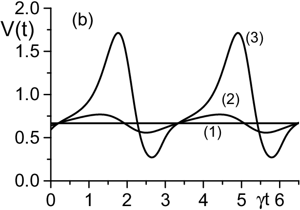
This result is illustrated in Fig. 2a for the different levels of modulation and for $f_{1}=0$ reaches to the standard result $n^{out}=2\gamma(f_{0}-f_{th})/k$. Let us turn to study the entanglement on the formula (12), which for $f_{1}=0$ also coincides with an analogous one for the ordinary NOPO. Typical results for $\varepsilon\left(t\right)=\frac{k}{\gamma_{3}}\left(f_{0}+f_{1}\cos\left(\delta t\right)\right)$ are presented in Fig. 2b for the above-threshold regime. The variance is seen to show a time-dependent modulation with a period $2\pi/\delta$. The drastic difference between the degree of two-mode squeezing/entanglement for modulated and stationary dynamics is also clearly seen in Fig. 2b. The stationary variance (curve 1) near the threshold having a limiting squeezing of $0.5$ (see also Fig. 3a, curve 1) is bounded by quantum inseparability criterion $V<1$, while the variance for the case of modulated dynamics obeys the EPR criterion $V^{2}<1/4$ of strong CV entanglement for definite time intervals. The minimum values of the variance $V_{min}=V\left(t_{m}\right)=V^{out}(t_{m})/2\gamma$ and corresponding photon numbers $n_{min}=n_{0}(t_{m})$ of Figs. 2 at fixed time intervals $t_{m}=t_{0}+2\pi m/\delta$, ($m=0,1,2...$) are shown in Figs. 3. As it is expected, the degree of EPR entanglement increases with ratio $f_{1}/\overline{f}$. The production of strong entanglement occurs for the period of modulation comparable with the characteristic time of dissipation, $\delta\approx\gamma$ and dissapears for asymptotic cases of slow ($\delta\ll\gamma$) and fast ($\delta\gg\gamma$) modulations.

(ii) Model of periodically pumped NOPO. We turn now to the scheme of Fig. 1 subjected by a periodic sequence of identical laser pulses. We consider a rectangular form of the pulses of the duration $T_{1}$ assuming that $T_{1}$ is much less than the interval $T_{2}$ between the pulses. Period averaged pump field amplitude $\overline{f}=f_{L}T_{1}/(T_{1}+T_{2})$, where $f_{L}$ is the highness of laser pulses, and hence the above-threshold regime is realized if $f_{L}T_{1}>\frac{\gamma\gamma_{3}}{k}(T_{1}+T_{2})$. The mean photon numbers and the variance $V(t)$ are calculated on the formulas (4) and (12). The predictions of the numerical calculations are shown on Figs. 4 for one of the preferable regimes (for typical $\gamma=10^{6}s^{-1}$, $T_{1}=10^{-8}s$ and the repetition rate $T_{2}^{-1}=1MHz$). It is clearly evident from Fig. 4a the mean photon number increases during laser pulses and decays during the interval $T_{2}$ between pulses due to dissipation in the cavity. One can conclude from Fig. 4b that the weak entanglement criterion $V<1$, is fulfilled for any time intervals. However, we have also found remarkable result that the variance goes below the inseparability level of $0.5$ in the ranges of maximal photon numbers, for appropriate chosen parameters. It has occurred for non-stationary regime, if $T_{1}$ is enough shorter than the relaxation time and hence the dissipative effects in modes dynamics are still unessential. We illustrate these results by calculation of the minimum values $V_{min}$. Considering for simplicity NOPO below and near the threshold and assuming $T_{1}\ll T_{2}$, we get from Eq. (12)

where $\varepsilon_{L}=f_{L}k/\gamma_{3}$. This formula is in accordance with the data of Fig. 4b. As we see the degree of EPR entanglement increases with $\varepsilon_{L}T_{1}$.

It is well known that the linearized theory is applicable only outside the critical region, although the variance (12) is surprisingly well defined also at the threshold. As our analysis shows, the condition of the validity of linear results for the near-threshold regimes reads as $\left|\overline{f}/f_{th}-1\right|\gg\left(\lambda/\gamma\right)\exp\left[2(f_{1}/f_{th})(\gamma/\delta)\right]$ for the system (i), while for (ii) the condition takes more simple form $\left|\overline{f}/f_{th}-1\right|\gg\left(\lambda/\gamma\right)$. For typical $\lambda/\gamma\ll 1$, both conditions are fairly easy to satisfy even for narrow critical ranges. Note, that the accuracy of our analytical calculations has been verified by the numerical simulations based on the quantum state diffusion method.

In conclusion, we note that both schemes (i) and (ii) operate under non-stationary conditions that has a significant impact on formation of high-degree CV entanglement even in the presence of dissipation and cavity induced feedback. We stress that the properties of periodically pulsed entanglement can be widely controlled via the modulation parameters. We would like to point out also that time-dependent output variance could be observed by means of time-resolved homodyne measurements Wenger; Wenger1. We believe that the results obtained are applicable to a general class of quantum dissipative systems and can serve as a guide for further studies of entanglement physics in application to time-resolved quantum information protocols.