On Quantum A/D and D/A Conversion
Abstract
An algorithm is proposed which transfers the quantum information of a wave function (analogue signal) into a register of qubits (digital signal) such that qubits describe the amplitudes and phases of points of a sufficiently smooth wave function. We assume that the continuous degree of freedom couples to one or more qubits of a quantum register via a Jaynes Cummings Hamiltonian and that we have universal quantum computation capabilities on the register as well as the possibility to perform bang-bang control on the qubits. The transfer of information is mainly based on the application of the quantum phase-estimation algorithm in both directions. Here, the running time increases exponentially with the number of qubits. We pose it as an open question which interactions would allow polynomial running time. One example would be interactions which enable squeezing operations.
I Introduction
Traditionally quantum computing and quantum cryptography have been formulated in a digital setting, i.e. with qubits NC. However, also models with continuous variables have been proposed ContinuousLloyd. Protocols for continuous variable cryptography have been investigated in detail (e.g. Silberhorn). In loyll several operations on hypothetical continuous variable quantum computers have been proposed which can generate arbitrary unitaries. The author argues that continuous models possess various advantages compared to the standard model quantum computer. Therefore an interface between continuous and discrete registers is desirable, since with this device one could combine the advantages of both approaches. There are also other reasons why the bridge between continuous and discrete degrees of freedom is an interesting issue of research: The possibility to transfer the wave function of a massive particle or the state of a light mode to a quantum register would allow to use algorithmic measurement schemes like those proposed in deck for POVM measurements on the continuous degree of freedom. Similarly, the ability to transfer quantum information from digital to analogue would allow to use state preparation algorithms in quantum computers Soklakov for algorithmic state generation in the analogue system. Furthermore, the implementation of POVM measurements with an uncountable number of outcomes on a finite dimensional system is only possible if one couples it to a continuous degree of freedom Ariano.
An interesting system where the state of a light field is transfered to the state of many two-level systems and vice versa is the micromaser (see wellens and references therein). The two-level atoms cross a cavity one after another such that at most one atom is present in the cavity at any time. While it is passing the cavity, each atom is interacting with the cavity field mode via a Jaynes Cummings Hamiltonian. One can prove wellens that every state of the field mode can asymptotically be prepared as a limit if an infinite number of atoms, initialized to an appropriate state, passes the cavity. It has been shown that for many interesting examples small numbers of atoms are sufficient to prepare the desired state with high fidelity. Since the final state of the field in the asymptotic scheme does not depend on its initial state, the latter has been completely transferred to the outgoing atoms. Therefore the system realizes asymptotically the transfer of quantum information in both directions. However, the fact that these statements refers to asymptotic behaviour indicates already that the state is typically not encoded on a minimal number of atoms.
Another system where quantum state transfer between a multi-photon state and the states of atoms and vice versa has already been experimentally implemented is described in Polzik. In this “quantum memory for light” the eigenvalues of the total spin operator of the atoms define the basis states of the atomic memory. However, this scheme encodes an -photon states in a collective polarization of an atom ensemble where the number of atoms is also of the order , i.e., the number of qubits is in the order of the dimension of the encoded space. In this article we propose a quantum analogue-to-digital converter where the number of qubits needed grows only logarithmically in the dimension of the encoded space for the cost of an exponential running time of the algorithm. We shall discuss later whether this shortcoming can be removed. The question of the cost of accurate A/D conversion is directly connected with the question of the computational power of analogue computers, which is already an interesting problem in classical computer science Vergis. Whether or not a continuous degree of freedom could be used to store a “reasonable number” of qubits depends on the ability to access a subspace of exponentially large dimension on a “reasonable” time scale.
Here the continuous degree of freedom is represented mathematically by the Hilbert space , the set of square integrable functions on the real line. It is isomorphic to , the space of square summable sequences over by choosing the eigenfunctions of a harmonic oscillator as complete orthogonal system. This shows that continuity or discreteness is here not a property of the Hilbert spaces but rather of the considered observables. Our A/D and D/A converters refer explicitly to a discretization with respect to a a variable with continuous spectrum, e.g. the position variable of a Schrödinger particle, but also applies to the formally equivalent variables of a light mode. Using the above isomorphism , it would be straightforward to transfer the information such that the state with oscillation quanta is mapped onto the th binary word in the discrete register. However, here we would like to represent the values of the wave functions at points directly by the coefficients of the binary words of the discrete register. For doing so, we restrict us to Schrödinger wave functions that are contained in the interval (except e. g. exponential tails). The -qubit register is represented by with basis states with . Then we demand that every sufficiently smooth wave function is converted to the quantum register state
| (1) |
in an approximative sense. We will show below that ”sufficiently smooth” means that the norm of the derivative of the wave function is not too large. The conversion operations that we will use are unitary transformations on
Now we describe the model in which conversion from analogue to digital is possible. This provides us with the available resources for the conversion algorithm.
We assume that the interaction is described by the Jaynes Cummings Hamiltonian CBla
| (2) |
where is the interaction strength and we have used the conventions
| (3) |
where denotes the Pauli matrix acting on qubit and and are the position and momentum operators, respectively, defined by
We can rewrite the Hamiltonian in eq. (2) as
| (4) |
Note that we choose the oscillator parameters such that and set throughout the paper. The Hamiltonian (2) appears often in physical systems when the continuous degree of freedom is an harmonic oscillator, e.g., an oscillation mode of ions in a trap CBla; CZ.
To achieve A/D conversion it is not sufficient to use just Hamiltonian evolution with Hamiltonian (4), we will also need various other unitary operators. For example, below we want to use the terms and of eq. (4) separately. Fortunately, there exists already a well–developed technique which allows to simulate various effective Hamiltonians ernst; Zanardi. Propagating the system only for short time intervals with the Hamiltonian (4) and interrupting this by one qubit unitaries, we can cancel or modify terms of the Hamiltonian. We use the fast control limit (also called bang–bang control), i. e. Hamiltonian evolution is neglected during one qubit operations are applied. In section III we will explicitly outline the one qubit operations and pulse sequences that entail the desired modifications of the Hamiltonian. Finally, as our last resource we assume that on the quantum register, we have the ability of universal power of quantum computation. Even though we use a specific interaction between continuous and discrete register as a resource for the conversion algorithm there are several generalizations which will be obvious after having discussed our method. First, the particle wave needs not necessarily interact with all qubits simultaneously and with the same strength, one could also have different coefficients. We will furthermore see that the only requirement is that one of the interactions and can be simulated, because the other can be obtained by implementing a Fourier transform to the continuous system.
We now describe the organization of this article. In section II we explain the algorithm that achieves the conversion of quantum information. Each step of the algorithm is given with its corresponding operator that acts on the tensor space of qubit register and wave function. In section III we describe the procedures for simulation of Hamiltonians which generate the required effective Hamiltonians from the given one. In section IV we describe briefly that the time reversed implementation can in principle be used for a digital to analogue converter. We summarize and discuss our results in section V. The appendix gives a proof of eq. (31).
II The A/D conversion algorithm
We first sketch the general idea of the functioning of the A/D converter. It uses a variant of the standard phase estimation algorithm ClevePhase; NC in order to bring the wave function amplitudes into the appropriate place of the qubit register (cf. the scheme of eq. (1)). The essential principle is that the interaction implements a controlled- operation which allows to use the qubit register als “measurement apparatus” for . After this procedure the joint quantum state displays a high degree of entanglement between its qubit and its wave function part. Therefore, in a final step we displace – depending on the value of the qubit register – all parts of the wave function to the same location, so that all quantum information is deleted in the continuous Hilbert space and transferred to the qubit register (again, in an approximate sense). The controlled displacement is done by a interaction.
Before we start the conversion process the phonon wave function is contained in the interval . Here the length should be estimated in such a way that the substantial part of the wave function is contained in this interval. We start with the following product state
| (5) |
To make subsequent procedures simpler we displace the wave function an amount of to the right such that the new wave function lies in the interval . The displacement operator that achieves this is
| (6) |
As will be recalled in section III we can cancel unwanted terms in eq. (4) by standard decoupling techniques by interspersing the natural evolution with one qubit control operations.
| (7) |
The application of this operator to the joint state (cf. eq. (5)) of qubits and wave function yields
| (8) |
A comparison with formula (6) shows that by choosing the time span we can realize the desired displacement of the wave function. The displaced state is denoted by .
In the first part of the phase estimation algorithm the qubits are in a uniform superposition of computational basis states and control the application of the operator to the wave function. This can be formulated as
| (9) |
where operator is given as
| (10) |
Here is the projection operator that acts on the th qubit of the qubit register defined by
| (11) |
Unfortunately, we cannot implement the operator as it is with our available resources. But since in eq. (11) can be written as , we can split into two factors
| (12) |
The second factor acts only on the wave function multiplying it with a position–dependent phase. Therefore eq. (9) is equal to
| (13) |
We can realize this transformation in the following three steps
- i)
- ii)
-
To bring the qubit register into the uniform superposition of all computational basis states we apply to each qubit the operator
since
(17) - iii)
-
The structure of the operator as defined in eq. (12) is very similar to the one of the operator of eq. (15). The only difference are the factors in the exponent of . Clearly we cannot increase the strength of the interaction by any selective decoupling scheme. In order to obtain a unitary which would correspond to the exponentially growing interaction we need exponential interaction time (see section III).
After the application of these steps the quantum state of the joint system is changed to
| (18) |
Note that we have preferred to use the notation even though position eigenstates do not exist (readers who appreciate mathematical rigor may forgive us). The whole expression is nevertheless a well-defined state in the joint Hilbert space. The second part of the phase estimation algorithm consists of the application of an inverse Fourier transform to the qubit register. The Fourier transformation (and its inverse) can be efficiently implemented on a quantum computer Cop; NC. After this transformation the quantum state becomes
| (19) | |||||
displays a high degree of entanglement between its qubit and its wave function part. The following procedure removes a large part of this entanglement and thus completes the transfer of quantum information. For this purpose we apply the following operator to the quantum state
| (20) |
As before we will discuss the implementation of this operator with our resources in section III. Acting with operator on the quantum state of eq. (19), the wave function part is displaced where the amount depends on the entangled qubit state
| (21) | |||||
where we have used the quantity
| (22) |
Making the substitution we can rewrite this quantum state as
| (23) |
where
| (24) |
The function is periodic with period . One can easily show that
| (25) |
Besides, the function becomes highly peaked around for a large number of qubits as shown in fig. 1. In fact, the width of is proportional to . Outside the peak the function takes on values that have only a small modulus (). Thus the wave function part in the quantum state of eq. (23) displays a peak around where (cf. its definition in eq. (22)) is approximately the mid point of the interval .
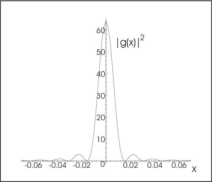
The result in eq. (23) is almost satisfactory, but a minor technical point should be mentioned. We would like that in eq. (23) each qubit register state has the same ”wave function” in its corresponding continuous part of the tensor space. We have seen that the function can be neglected outside its peaks. Considering the –dependent integration bounds in eq. (23), the relevant wave function is not the full peak of only for low and high values of . Hence we have to make the additional assumption for the original wave function that holds in the two subintervals of length that join the end points and of the interval .
Using this technical assumption and the fact that can be neglected far away from its peak, we can rewrite the quantum state of eq. (23) to a very good approximation as
| (26) |
where is some multiple of the width of the function and hence . Eq. (26) shows that now the quantum information has been transferred to the qubit register, since the continuous Hilbert space is left with the ”standard wave function” . This is in accordance with the no cloning theorem NoCloning that precludes the copying of quantum information.
The result eq. (26) still shows some degree of entanglement as qubit and wave function part are connected via the integration over . In order to assess the magnitude of this entanglement, we calculate the reduced density operator of the qubit register
| (27) | |||||
In the following we show that for a large number of qubits this density operator can be replaced by the density operator
| (28) |
which is the density operator of a pure state with
| (29) |
The constant ensures the correct normalization in eqs. (28) and (29). To demonstrate the possibility of replacing by , it is appropriate to consider the trace norm 11 1 The trace norm of an operator is defined as . of the difference operator . For – thanks to Hölder’s inequality – we can bound expectation values for an observable as
| (30) |
where is the operator or spectral norm of . In the appendix to this article we show the following bound for the trace norm
| (31) |
where
| (32) |
Eqs. (30) and (31) show that in the limit of a large number of qubits the density operators and are equivalent for all observables whose norm diverges slower than . We thus need a large number of qubits in order to represent the quantum information of a wave function faithfully in a qubit register. Furthermore, according to eq. (32) the accuracy of this representaion is also determined by the norm of the derivative of the wave function. Hence the smaller the derivative of the wave function, the better works its conversion into digital information (for a fixed number of qubits).
We have already mentioned that the time needed for the execution of the phase estimation algorithm grows exponentially with the number of qubits. Thus there is a trade–off between accuracy and speed for our A/D conversion algorithm. Squeezing operations squeez1; loudon, i. e. operators of the form
| (33) |
could speed up the phase estimation algorithm considerably. For, the squeezing operator could magnify the wave function by a factor while preserving its shape. This would decrease the time for phase estimation by a factor . Note that we can rewrite as
| (34) |
In order to generate such unitaries we have to simulate the Hamiltonian
To achieve this, we observe that
We conclude that can be obtained by the following second-order simulation scheme which applies the following Hamiltonians for a small time :
| (35) |
Up to terms we obtain a time evolution according to the desired Hamiltonian multiplied with a slow-down factor provided that the qubit is set to the state . Due to
one could simulate exponentially large interaction time by a linear number of concatenated squeezing operations before the interaction has taken place and undoing the squeezing afterwords. However, the problem with a second-order simulation is that the running time increases with the desired accuracy. Since the required error decreases exponentially with the desired qubits we expect here also exponential running time. However, on a scale where squeezing operations are available with sufficient accuracy one could nevertheless expect a speed up.
III Selective Decoupling and Simulation of Hamiltonians
Simulation of Hamiltonians by interspersing the natural time evolution with fast control operations is used in NMR since decades ernst. These techniques are subject of many theoretical investigations Zanardi; VKL99; GraphPawel. Here we refer only to very basic ideas.
Let be the natural Hamiltonian (2). Using the anti commutator relation between Pauli matrices
| (36) |
we get the equation
| (37) |
where
| (38) |
The operators and do not commute, but for a small time interval we can use the Baker Campbell Hausdorff formula
| (39) |
where
| (40) |
Thus to leading order in the unwanted terms have canceled each other.
Therefore, if during a time interval we change frequently between Hamiltonian evolution and the product of one qubit operations , we can realize the unitary operator
| (41) |
In the language of GraphPawel we have now “simulated the Hamiltonian”
In a similar way, we can also select the term with in (2) by applying -rotations to all qubits. Complete decoupling can be achieved if we apply to all spins since this reverses the sign of the and the term. If we want to cancel all terms except from the interaction
| (42) |
for one specific qubit we apply to qubit and to all the other qubits. To simulate the time evolution
we may concatenate the commuting unitaries
which are obtained by applying the simulated interaction (42) on a time interval of length . If we apply arbitrary single qubit unitaries to qubit initially and apply afterwords, we obtain the time evolution
This shows that we can replace the Pauli matrix in eq. (42) by other Pauli matrices or by as we like.
IV Digital-Analogue Conversion
Using the results of the previous sections, we can easily describe an algorithm for digital-analogue conversion. Roughly speaking, the argument is as follows. Let be the transformation on the continuous and the discrete degrees of freedom which implements the complete analogue-digital conversion algorithm. Provided that the wave function was sufficiently smooth the system ends up almost in the product state
| (43) |
where is a superposition state with coefficients with as defined in eq. (29) and is the function whose absolute square was plotted in fig. 1 translated by . If we apply to the state (43) we obtain hence almost the original wave function . It is clearly required that the values correspond to some sufficiently smooth wave function. We have explained that sufficiently smooth means here that is small enough. Hence the vector corresponds to a smooth wave function whenever the values do not vary too much for adjacent .
In order to obtain definite accuracy bounds from this idea we recall that the reduced state of the discrete register satisfies
| (44) |
If we set in eq. (30), we obtain
| (45) |
Hence the largest eigenvalue of is at least . Let
| (46) |
be the Schmidt decomposition of the exact bipartite state after the conversion. Then the absolute square of the dominating coefficient is the largest eigenvalue of the reduced density operators on both subsystems. Hence the square of the norm distance between and is at most . It follows that the error which arises from replacing the joint state by the tensor product state
| (47) |
is of the order . We know furthermore that we may replace the state of the digital system by such that the error in trace norm is in the order of . We conclude that applying to
| (48) |
leads to the wave function up to a trace norm error in the order of . The initialization of the continuous system to the state is clearly a non-trivial task. It is some wave packet which is similar to the function translated by . To construct algorithms which work also for more general initializations shall not be our subject here.
V Conclusions
In this article a quantum algorithm has been outlined that can read in the quantum information of a wave function into a qubit register. This can be viewed as the quantum analogue of an A/D converter which encodes an -dimensional system obtained by discretization of a continuous wave function into a qubit register.
The principal ingredient for the A/D converter is the use of the phase estimation algorithm that is already popular for other purposes in quantum computing. The principal resources are interaction Hamiltonians which are tensor products of a position or a momentum operator with a Pauli matrix of the discrete system. Effective Hamiltonians of this type can for instance be obtained from the Jaynes Cummings Hamiltonian using standard techniques for selective decoupling.
Whether the proposed A/D and D/A converters could be realized depends on the one hand on the experimental progress. On the other hand and perhaps even more important, further theoretical work is required to investigate more systematically the advantages that arise when one combines discrete and continuous degrees of freedom in quantum computing.
Acknowledgment
The authors are grateful to the Landesstiftung Baden–Württemberg that supported this work in the program ”Quantum-Information Highway A8” (project ”Kontinuierliche Modelle der Quanteninformationsverarbeitung”). This work has been completed during DJ’s visit of Hans Briegel’s group at IQOQI in Innsbruck, whose hospitality is gratefully acknowledged.
Appendix
In this appendix we prove eq. (31). To simplify the notation we set . We start with the density operator and use the mean value theorem in eq. (27)
| (49) |
and analogously for the conjugate function . Therewith we can write the matrix elements of the difference operator in the standard basis as 22 2 In the limit the normalization factor can be neglected.
| (50) | |||||
We can rewrite this expression in an operator form
| (51) |
where the dimensional vectors and are defined in the standard basis as
| (52) |
Using the triangle inequality, eq. (51) leads to the following estimate for the trace norm
| (53) |
We now consider the trace norm of the operator
We see from this formula that the operator acts non–trivially only on the two dimensional subspace . Choosing an ONB for this subspace with ( is the Euclidean norm), we arrive at the following matrix representation for
| (54) |
where is a unit vector. From eq. (54) the trace norm of can be bounded uniformly
| (55) |
In addition, for we can evaluate the Euclidean norms of the vectors and approximately as
| (56) |
Using the results of eqs. (55) and (56), we can bound the difference between the two density operators as
| (57) |
Since for the width and thus
| (58) |
the inequality (57) establishes the bound eq. (31) with the constant
| (59) |
References
- (1) M. Nielsen and I. Chuang. Quantum Computation and Quantum Information. Cambridge University Press, 2000.
- (2) S. Lloyd and S. Braunstein. Quantum computation over continuous variables. Phys. Rev. Lett., 82(8):0031–9007, 1999.
- (3) Ch. Silberhorn, T. C. Ralph, Lütkenhaus N., and Leuchs G. Continuous variable quantum cryptography: beating the 3 db loss limit. Phys. Rev. Lett., 89:167901, 2002.
- (4) S. Lloyd. Hybrid quantum computing. arXiv:quant-ph/0008057, 2000.
- (5) T. Decker, D. Janzing, and M. Rötteler. Implementation of group-covariant positive operator valued measures by orthogonal measurements. J. Math. Phys., 46:012104, 2005.
- (6) A. Soklakov and R. Schack. Efficient state preparation on a quantum computer. arXiv:quant-ph/0408045, 2004.
- (7) G. D’Ariano, P. Lo Presti, and M. Sachi. A quantum measurement of the spin direction. Phys. Lett. A, 292:233, 2002.
- (8) T. Wellens, A. Buchleitner, B. Kümmerer, and H. Maasen. Quantum state preparation via asymptotic completeness. Phys. Rev. Lett, 85:3361–3364, 2000.
- (9) J. Sherson, B. Julsgaard, I. Cirac, J. Fiurasek, and E. Polzik. Experimental demonstration of quantum memory of light. Nature, 432:482–486, 2004.
- (10) A. Vergis, K. Steiglitz, and B. Dickinson. The complexity of analogue computation. Math. Comput. Simulation, 28:91–113, 1986.
- (11) J. I. Cirac, R. Blatt, A. S. Parkins, and P. Zoller. Preparation of Fock states by observation of quantum jumps in an ion trap. Phys. Rev. Lett., 70:762–765, 1993.
- (12) J. I. Cirac and P. Zoller. Quantum computation with cold trapped ions. Phys. Rev. Lett., 74:4091–4094, 1995.
- (13) R. R. Ernst, G. Bodenhausen, and A. Wokaun. Principles of nuclear magnetic resonance in one and two dimensions. Clarendon Press, Oxford, 1987.
- (14) P. Zanardi and S. Lloyd. Universal control of quantum subspaces and subsystems. Phys. Rev. A, 69:022313, 2004.
- (15) R. Cleve, A. Ekert, C. Macchiavello, and M. Mosca. Quantum algorithms revisited. Proc. Roy. Soc. London A, 454:339–354, 1998.
- (16) D. Coppersmith. An approximate Fourier transform useful in quantum factoring. Technical report, IBM RC 19642, 1994.
- (17) W. Wootters and W. Zurek. A single quantum bit can not be cloned. Nature, page 802, 1982.
- (18) D. Stoler. Generalized coherent states. Phys. Rev. D, 4:2309–2312, 1971.
- (19) R. Loudon and P. L. Knight. Squeezed light. J. Mod. Optics, 34:709–759, 1968.
- (20) L. Viola, E. Knill, and S. Lloyd. Dynamical decoupling of open systems. Phys. Rev. Lett., 83:2417–2421, 1999.
- (21) P. Wocjan, D. Janzing, and T. Beth. Simulating arbitray pair-interactions by a given Hamiltonian: graph-theoretical bounds on the time complexity. Quant. Inf. & Comp., 2:117–132, 2002.