From quantum graphs to quantum random walks
Abstract
We give a short overview over recent developments on quantum graphs and outline the connection between general quantum graphs and so-called quantum random walks.
1 Introduction
The study of quantum mechanics on graphs has become an important tool for investigating the influence of classical dynamics on spectra, wavefunctions and transport properties of quantum systems. Quantum networks have been used with great success to model quantum phenomena observed in disordered metals and mesoscopic systems (Chalker and Coddington 1988); typical behaviour found in diffusive systems such as localisation - delocalisation transitions (Freche et al 1999), transport properties (Pascaud and Montambaux 1999) and quantum spectral statistics (Klesse and Metzler 1997) have been studied on graphs in the limit of infinite network size. Kottos and Smilansky (1997, 1999) looked at quantum graph models for general, non-diffusive graphs; this approach was motivated by trying to understand the validity of the Bohigas-Giannoni-Schmit (BGS) conjecture (Bohigas et al 1984) in terms of periodic orbit trace formula. The conjecture relates the properties of the classical dynamics of a systems to the spectral statistics of its quantum counterpart and states that for chaotic systems the statistics depends only on the symmetries of the problem and follows random matrix theory (RMT) otherwise.
Making use of the fact that periodic orbit trace formula are exact on quantum graphs and that there are only a finite number of different length scales on a finite graph, a series of remarkable results have been obtained over the last couple of years. A closed form quantisation conditions in terms of periodic orbits has been given by Blümel et al (2002); Barra and Gaspard (2000) derived an integral expression for the level spacing distribution starting form the periodic orbit trace formula. Furthermore, Schanz and Smilansky (2000) described localisation on one-dimensional chains in terms of combinatorial expression using periodic orbits. The most far reaching development is maybe due to Berkolaiko et al (2002,2003), who, inspired by work from Sieber (2002) and Sieber and Richter (2001), derived next to leading oder terms for the formfactor. Extensions to all orders have been given by Müller et al . (2004). Gap conditions given by Tanner (2001) and Gnutzmann and Altland (2004) give lower and upper bounds for the border of universality. For a recent review on quantum graphs see Kuchment (2002).
Quantum dynamics on graphs became an issue also in the context
of quantum information. Aharonov et al (1993)
pointed out that a random quantum walk on one dimensional chains can be faster
than the corresponding classical random walk. Since then, a whole field
has emerged dealing with quantum effects on graphs with properties superiour
to the corresponding classical operations. For an introductory overview
and further references, see Kempe (2003).
We will in the following give a general definition of quantum graphs and discuss a specific set-up considered by Kottos and Smilansky (1997). We will then review recent developments on the spectral statistics of quantum graph ensembles. Next, we discuss a special class of quantum graph ensembles, so-called regular quantum graphs. These types of graphs can show strong deviations from RMT depending on topological properties imposed on the graph in form of edge-colouring matrices. We will show that such graphs can be interpreted as realisations of quantum random walks on graphs.
2 Quantum graphs - a brief review
2.1 Quantum graphs on line graphs
In its most general form, a quantum graph is defined in terms of a (finite) graph together with a unitary propagator ; it describes the dynamics of ”wavefunctions” on the graph according to
such that waves can propagate only between connected vertices. Motivated by physical application we will adopt a construction of quantum graphs in terms of so-called line-graphs as explained below.
A (finite) directed graph or digraph consists of a finite set of vertices and a set of ordered pairs of vertices called arcs. We denote by and the set of vertices and arcs of the digraph , respectively. Given an ordering of the vertices, the adjacency matrix of a digraph on vertices, denoted by , is the -matrix where the -th element is defined by
| (1) |
An undirected graph (for short, graph) is a digraph whose adjacency matrix is symmetric. The undirected connections between vertices are called edges in this case. The line digraph of a digraph , denoted by , is the graph which is obtained when taking the arcs as the new vertices; it is thus defined as and, given , the ordered pair if and only if (Bang-Jensen and Gutin 2001).
A quantum graph associated with a digraph on vertices can then be defined in terms of a set of unitary vertex scattering matrices on vertices and a set of arc lengths defined for every arc . Waves propagate freely along the directed arcs, transitions between incoming and outgoing waves at a given vertex are described by the scattering matrix , see Fig. 1a. The two sets specify a unitary propagator of dimension defining transitions between arcs which has the form (Kottos and Smilansky 1997)
|
(2) |
where is a wave number and
|
(3) |
The local scattering matrices describe the underlying physical process which may be derived from boundary conditions on the vertices. We will construct an example below but may often regard the ’s as arbitrary unitaries. Let and be the number of incoming and outgoing arcs of a vertex , respectively. A sufficient and necessary condition for a digraph to be quantisable in the way above is then, that for every vertex , (Pakoński et al 2003). This means in particular that if is an undirected graph then it is quantisable.
Kottos and Smilansky (1997) considered solving the 1d Schrödinger equation on an undirected graph assuming free propagation on the arcs and imposing continuity and flux conservation at the vertices. The solution on each arc propagating from vertex takes on the form
with being the outgoing or incoming wave at vertex or . Continuity and flux conservation can then be written in terms of the amplitudes and at the vertices, that is
| Continuity: | ||||
| Flux cons.: |
These conditions give rise to local scattering matrices mapping amplitudes onto at vertex having the form
| (4) |
The eigenvalue condition is then given as
| (5) |
with as defined in (2), (3). Scattering matrices for more general boundary conditions can be found in Kottos and Smilansky (1999).

The ”classical” dynamics corresponding to a quantum graph defined by a unitary propagator is given by a stochastic process with transition matrix defined by
| (6) |
The matrix is clearly stochastic, as due to the unitary of ; the set of transition matrices related to a unitary matrix as defined in (6) is a subset of the set of all stochastic transition matrices, referred to as the set of unitary-stochastic matrices. The topology of the set in the space of all stochastic matrices is in fact quite complicated, see Pakoński et al (2001). In what follows, we will only use that has a largest eigenvalue 1 with corresponding eigenvector which follows from the Frobenius-Perron theorem and being unitary-stochastic.
Note that both the quantum mechanics as well as the associated stochastic dynamics relates to transitions between arcs and is thus defined on the line digraph of .
2.2 Unitary stochastic ensembles and spectral statistics
Inspired by the BGS conjecture for quantum systems, we expect a link between the dynamical properties of the stochastic process and the statistical properties of the spectrum of associated unitary matrices . It is thus natural to consider the ensemble of unitary matrices
| (7) |
for a given graph and a fixed unitary stochastic matrix associated with a stochastic process on the line-graph of . Clearly, if for then it is for all . In fact, if all the arc length are incommensurate, sweeps out the space of unitary diagonal matrices of dimension . For practical purposes we will thus often replace averages over a given by averaging over the space of diagonal unitary matrices with using the Euclidean measure on the - torus.
Rather than looking at the spectrum obtained from the secular determinant (5), we will here consider the spectrum for fixed wavenumber and than average over . One can write the spectrum in terms of a periodic orbit trace formula reminiscent to the celebrate Gutzwiller trace formula being a semiclassical approximation of the trace of the Green function (Gutzwiller 1990). We write the density of states in terms of the traces of , that is,
| (8) |
where refers to the eigenphases of . The traces can be given as sum over all periodic paths of length on the graph, i.e.
Describing a given periodic path in terms of its vertex code , with being an allowed transitions between vertices, one obtains for the amplitudes and lengths
| (9) |
where the amplitudes give again transitions between arcs (not vertices). An example of such a periodic path is given in Fig. 1b.
Trace formulas like (8) are a starting point for analysing the statistical properties of quantum spectra. The statistical quantities such as the two-point correlation function can be written in terms of the density of states , that is,
| (10) |
where is the mean level density. The average is taken here over the angle as well as over the USE (which is equivalent to energy averaging). The Fourier coefficients of (10) can be written in terms of the traces of ; one obtains
| (11) |
with and the average is taken over a USE. The so-called form factor can thus be written as a double sum over periodic paths on the graph
| (12) | |||||
| (13) |
The first term in (13), also called the diagonal term (Berry 1985), originates from periodic orbit pairs () related through cyclic permutations of the vertex symbol code. There are typically orbits of that kind and all these orbits have the same amplitude and phase . The corresponding periodic orbit pair contributions is (in general) - times degenerate where is the length of the orbit and is a symmetry factor ( for time reversal symmetry).
Expanding the random matrix result for the formfactor, one obtains for
The linear terms are reproduced by the diagonal contribution which gives the important link between the stochastic dynamics and the spectral statistics; it follows from given there is a gap between the leading and next-leading eigenvalue of . Contributions to the double sum in (13) which survive the ensemble average are due to periodic orbit pairs where orbits visit the same arcs along its path but in different order. The simplest examples are ”figure eight” orbits of the type shown in Fig. 2 which arise in undirected graphs. Berkolaiko et al (2002) could indeed show that orbits of that type give the correct - contributions to the GOE - form factor. In fact, a general scheme emerges relating contributions to periodic orbits with intersections. This work was inspired by a similar analysis for general quantum systems by Sieber and Richter (2001). The periodic orbit contributions giving the have been worked out by Berkolaiko et al (2003) and a general scheme for obtaining higher order terms iteratively has been given by Müller et al (2004).

2.3 Border of universality
In the light of these recent developments, it becomes important to establish the boundaries at which the spectral statistics of quantum graph ensembles (or more general quantum systems) starts to deviate from random matrix behaviour. One can distinguish two different scenarios. Firstly, the properties of the underlying dynamics, that is, the stochastic process may be linked to the spectral statistics and may thus provide conditions for the onset of deviations from RMT behaviour; such an approach is in the spirit of the original BGS - conjecture making a connection between classical chaos and random matrix statistics. Secondly, one may consider special phase or length correlations in the quantum graph which could lead to interesting non-universal statistics; in this approach, quantum graph ensemble averages are carried out only over subsets of the full .
We will discuss known bounds on the border of universality related to the properties of the stochastic process. An interesting family of quantum graphs which belongs to the second category are so-called regular quantum graphs, which will be treated in more detail in section 3.
Spectral gap conditions
When studying the border of universality, we always need to consider the limit of large graphs, that is, . This limit is in general not well defined, but may often be obvious from the examples considered. We will thus define the semiclassical limit loosely via a family of unitary-stochastic transition matrices and associate ’s and take . The leading term in (13) then gives a condition for a family to show deviations from RMT statistics in terms of the spectrum of ; the diagonal term must obey
in order to match the leading coefficient in the expansion of the RMT form - factor; here is the spectral gap, that is, with being the next to leading eigenvalue of ) and is fixed. The condition above implies that we expect to see deviations from RMT behaviour to leading order if
that is, whenever the gap closes faster than for large system sizes (Tanner 2001). Based on super-symmetric techniques, Gnutzmann and Altland (2004) could give a lower bound by showing that the spectral gap condition guarantees RMT behaviour for . The border of universality must therefore lie in the range . Other bounds have been given by Berkolaiko et al (2002,2003) which have been derived from higher order terms in the expansion of the form factor. Below we we will give two examples families with displaying critical behaviour by neither converging to RMT nor to Poisson statistics in the semiclassical limit.
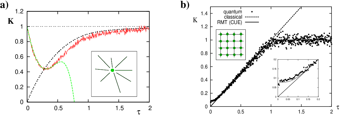
Quantum star-graphs:
Quantum star-graphs arise naturally when one quantises a graph with a single central vertex attached to undirected edges, see inset of Fig. 3a. The underlying graph is complete, that is, we can reach every edge from every other edge through the central vertex (ignoring the trivial dynamics on the outer vertices). Typical boundary conditions imposed on the wave equation at the central vertex following Kottos and Smilansky’s approach in Sec. 2.1 yield scattering matrices which greatly favour backscattering. The vertex scattering matrix (4) which is essentially equivalent to the matrix here is
| (14) |
The Markov processes associated with quantum star graphs correspond to systems of weakly coupled edges. Its dynamical properties are determined by the spectrum of the stochastic matrix associated with (14) which is highly degenerate and can be given explicitly (Kottos and Smilansky 1999), that is,
Quantum star-graphs have therefore a critical classical spectrum with a spectral gap vanishing proportional to ; one finds indeed spectral statistics intermediate between Poisson and COE statistics.
The two-point correlation function has been work out explicitly by Berkolaiko et al (2001) and has been shown to coincide with the statistics of so-called Seba billiards, that is, rectangular billiards with a single flux line. The first few terms in a power series expansion of the form factor have been derived by Kottos and Smilansky (1999) and Berkolaiko and Keating (1999) and yield
| (15) |
see Fig. 3a.
Diffusive networks:
The quantum mechanics of classically diffusive systems has been studied mainly in the context of Anderson localisation and localisation-delocalisation transitions, see e.g. Dittrich (1996) and Janssen (1998) for recent review articles.
As a simple example, we consider here a quantum graph corresponding to a classical Markov process on a regular lattice in dimensions, see Fig. 3b for . Choosing a stochastic matrix with constant transition probabilities between connected edges corresponds to -dimensional diffusion in the continuum limit ; here, is the number of vertices along each direction, that is, the total number of arcs is . Solving the diffusion equation with periodic boundary conditions allows one to recover the low lying part of the spectrum of , that is,
| (16) |
with diffusion constant and is a -dimensional integer lattice vector. The influence of the dimension on the small behaviour of the form factor in diffusive systems has been described in detail by, for example, Dittrich (1996) and references therein. In terms of the spectral gap condition, one obtains
that is, we expect universal statistics for only. (Actually, the bound by Gnutzmann and Altland (2004) guarantees random matrix statistics only for , numerics suggests however, that follows RMT already (Tanner 2001)). One finds convergence to the Poisson limit due to Anderson localisation in one dimension (Schanz and Smilansky 2000). The two-dimensional case is critical with which shows up in the form factor as a plateau for , that is, , see Fig. 3b (Tanner 2002).
3 Regular quantum graphs
In the following, we will consider quantum graphs for which the above bounds do not necessarily hold due to length correlations in the graphs, that is, averages are not taken over a full . We will actually look at a specific set of such non-generic quantum graphs, namely quantum graphs for which the global propagator consists of identical local scattering processes at every vertex. Such graphs have been called regular quantum graphs by Severini and Tanner (2004); the name derives from the notation regular graphs for graphs which have the same number of incoming and outgoing arcs at every vertex and thus share the property that vertices are locally indistinguishable. We will show that regular quantum graphs corresponding to the same underlying graph can behave very differently depending on how the local scattering processes are connected to each other. We will show that a crucial element in this is played by the possible ways regular graphs can be edge-coloured. Regular graphs are in fact another way at looking at quantum random walks as will be pointed out at the end of this section.
3.1 Regular quantum graphs and edge-colouring matrices
We will construct a quantum graph on a -regular digraph with vertices for which the wave dynamics at a given vertex of the graph is ”locally indistinguishable” from that of any other vertex of the graph. This is done by choosing a unitary -dim. matrix and a set of arc-lengths and ascribing the scattering process to every vertex in the graph with incoming as well as outgoing arcs chosen from the set of ’s at every vertex. This is done here by first fixing a so-called edge-colouring of the graph (see eg Bollobás 1979), that is, we assign one of different ”colours” to every directed arc of the graph in such a way that no vertex has two incoming or two outgoing arcs of the same colour. Note that there are many different ways to edge-colour a given regular graph for . Edge-colouring can be described in terms of a set of - dimensional permutation matrices having the property that
| (17) |
with being the adjacency matrix of ; the arc is then assigned the colour if the matrix element of is non-zero. We refer to the set of ’s as the edge-colouring matrices of 11 1 In Severini and Tanner (2004), these matrices have been called connectivity matrices.. In Fig. 4, an explicit example is shown with

The adjacency matrix of the line-graph of can then be written in the form (Severini 2003, Severini and Tanner 2004)
| (18) |
where is the matrix with all elements being equal to 1 and is the identity matrix. We proceed by defining a quantum graph on the line-graph of in the form of a unitary propagator as follows:
| (19) |
with and describing the local scattering process. The - dimensional matrix is also called the coin in the context of quantum random walks on graphs (Kempe 2003).
Note that different ways of edge-colouring the graph, that is, different decomposition of in the form (17) lead to different quantum graphs which may have quite different properties as will be shown in the next section; this is in contrast to the representations of the line-graph adjacency matrix (18) which are all equivalent up to relabeling the arcs in the graph. For modifications of this construction for undirected graphs with time reversal symmetry, see Severine and Tanner (2004).
3.2 From ’integrable’ to ’chaotic’ regular quantum graphs - some examples
In this section, we will show that different ways to edge-colour a graph can indeed lead to very different types of quantum graphs with spectral statistics ranging from Poisson to CUE. In other words, in regular quantum graphs it is the choice of the edge-colouring matrices , a purely topological quantity, which determines the properties of the quantum graph independent of the single vertex scattering processes given through the coin . We will demonstrate this here for a specific example, namely so called complete graphs with adjacency matrix , that is every vertex is connected to every other vertex, see Fig. 5. (Note that , here). A more general treatment can be found in Severini and Tanner (2004).

In the examples discussed below, we make use of the fact that for finite groups of order , we may write
| (20) |
where the ’s form a regular representation of . In what follows we will study various decompositions of and see how they effect statistical properties of the spectra of quantum graphs.
3.3 The cyclic group
We will first consider an abelian group, namely the cyclic group . The ’s forming a regular representation commute with each other and are of the form
|
The abelian nature of the group allows one to block-diagonalise the matrix into blocks of dimension each, independent of the coin . The spectrum of the quantum graph is then given by the spectra of the sub-matrices
The eigenvalues of are here characterised in terms of two quantum numbers, an ’angular momentum’ quantum number and a second quantum number counting the eigenvalues in each manifold. If the spectra for different are uncorrelated, one expects Poisson statistics of the total spectrum in the limit .
Figure 6a) shows spectral properties of with , that is, . We plot here the nearest neighbour spacing (NNS) distribution and the form factor . The coin is of the from where the local scattering matrix is choosen to be the Fourier matrix and the arc lengths entering the diagonal matrix are chosen independently and identically distributed in . The average is, for a fixed choice of the coin, taken by averaging over the wavelength . The numerical results are shown in Fig. 6a) and suggest indeed Poisson-statistics apart form deviations in the form factor on scales due to the ‘random nature’ of the coin.

3.4 The non-abelian case: the symmetric group
Next, we consider a specific example of a non-abelian group, namely the symmetric group with elements. By writing the permutation matrices forming the regular representation of in terms of the irreducible representations (for short irreps) of , we can again give the propagator in block-diagonal form where the blocks are now of size , with being the dimension of the irrep under consideration. The group has 2 one-dimensional, 1 two-dimensional and 2 three-dimensional irreps, and each - dimensional irrep is contained times in each according to the general formula
We thus have 5 independent sub-spectra making up the spectrum of the quantum graph of which two are of dimension , one is of dimension and two are of dimension ; the latter once are two and three times degenerate, respectively. The huge degeneracy in the spectra can clearly be seen in the spectral statistics; it is manifest in the peak at in , see Fig. 6b, and leads to
|
The spectra appear to be uncorrelated otherwise; note however, that the spectrum for each sub-block alone are correlated following statistics, which gives rise to the deviations from purely Poisson behaviour in (cf. dashed curve) as well as in the behaviour of the form factor for which is dominated by the sub-spectra of the three dimensional irreps.
3.5 The generic case: no symmetries
The overwhelming number of decompositions of the form (20) will of course have no common symmetry, that is, it is not possible to block-diagonalise the ’s simultaneously. We therefore do not expect any special features in the spectrum. The question remains, however, if the ’randomness’ put into the system by choosing a random edge-colouring is enough to produce generic, random matrix type, statistics. After all, these quantum graphs still possess a large degree of degeneracy due to the presence of identical coins at every vertex. A numerical study may thus reveal interesting insights into the range of validity of the RMT - regime. Fig. 6c shows the level statistics for an unstructured choice of edge-colouring matrices which is in good agreement with random matrix theory for the CUE - ensemble 22 2 Deviations in the formfactor for small can be attributed to the fact that the spectrum of itself is always contained in the full spectrum, see Severini and Tanner (2004); this part has been removed in the NNS statistic.. Note that the statistic has been obtained from the spectrum on an unitary matrix which has only non-zero elements of which only are independent; in addition, there are only different arcs lengths to choose from for different arcs. The origin of the universality in the spectral statistics in this type of quantum graphs is here clearly not due to the ’randomness’ in the choice of the matrix elements but due to random edge-colouring of the graph alone!
3.6 Quantum random walks
In recent years, the study of unitary propagation on graphs has also been looked at from the perspective of devising a quantum version of a random walk. This line of thought arose as part of the effort to build quantum information systems being able to do operations which are impossible or much slower on classical devices. It could indeed be shown that quantum random walks have this property under certain circumstances: quantum walks can be faster for some network geometries (Aharonov et al 1993) and can even lead to an exponential speed-up such as for the graph-traversal algorithm by Childs et al (2003); for an introductory overview and further references, see Kempe (2003). The generalisation of Grover’s algorithm (Grover 1997) to spatial searches on graphs (Shenvi et al 2003, Ambianis et al 2004, Childs and Goldstone 2004) is another remarkable recent result.
We will not study the properties of quantum random walks here; instead, we would like to point out that the discrete quantum walk modules discussed in the literature are in fact equivalent to regular quantum graphs such as introduced in the previous sections.
In brief, a discrete quantum random walk comprises of an in general - regular graph with vertices (where lattices are favoured in the literature) and a ’spin’ degree of freedom, where the spin can take up different states. A quantum state at a vertex with spin is then described by and the quantum wave function is a superposition of all possible vertex states. The quantum random walk consists of a ’walk’ element and a ’quantum coin toss’. The walk is steered by the internal spin states, that is, there exist matrices , which define in which direction the component is flowing, that is,
where the internal spin states remains unchanged. The ’s are obviously permutation matrices in the vertex space. The coin toss is simulated by applying a unitary transformation to the spin states at every vertex, that is,
the coin is unbiased, if throughout. It is clear from the construction, that one obtains a classical random walk on such a network, if one performs a measurement after every walk by projecting out the spin degrees of freedom.
A full cycle of walk and coin toss is then described by a unitary matrix
| (21) |
which has exactly the form of the propagator for regular quantum graphs in Eq. (19). We thus identify the ’s with the edge-colouring matrices and the coin is in fact a local scattering matrix. Writing the components of the wave function in notation is thus just a different way of labeling the arcs in the graph and the dynamics takes indeed place on the line-digraph of .
To demonstrate the mechanism, let us give a specific example: the quantum walk on an infinite line. A popular setting is the following walk:
| states: | ||||
| walk: | ||||
| coin: |
A random walk starting in the state then evolves according to
Continuing this process leads quickly to a probability profile which
grows linearly with the number of steps which is in contrast to the
classical spreading for 1d random walks being of the order
(Kempe 2003). It must be pointed out, however, that this is a pure symmetry
effect due the choice of edge-colouring matrices; in the setting
chosen here, the two operations and
commute. By introducing disorder into the quantum random walk on a line
by for example randomly switching the shift operation at every vertex
leads to a completely different behaviour resembling that of a quantum graph
on a diffusive network as discussed in sec. 2.3.
Acknowledgment:
The author would like to thank Simone Severine with whom some of the work reviewed here has been carried out. Thanks goes also to the Royal Society and Hewlett-Packard, Bristol, for financial support.
References
- [1] Aharonov Y, Davidovich L and Zagury N 1993 Phys. Rev. A bf 48 1687
- [2] Ambainis A, Kempe J and Rivosh A 2004 quant-ph/0402107.
- [3] Bang-Jensen J and Gutin G, Digraphs. Theory, algorithms and applications, Springer Monographs in Mathematics, Springer-Verlag, London, 2001.
- [4] Barra F and Gaspard P 2000 J. Stat. Phys. 101 283–320.
- [5] Bollobás B, Graph Theory - An Introductory Course Springer Graduate Texts in Mathematics, Springer-Verlag, New York, 1979.
- [6] Berkolaiko G and Keating J P 1999 J. Phys. A 32 7827.
- [7] Berkolaiko G, Bogomolny E B and Keating J P 2001 J. Phys. A 34 335.
- [8] Berkolaiko G, Schanz H and Whitney R S 2002 Phys. Rev. Lett. 88 104101.
- [9] Berkolaiko G, Schanz H and Whitney R S 2003 J. Phys. A 36 8373.
- [10] Berry M V 1985 Proc. R. Soc. A 400 229.
- [11] Bohigas O, Giannoni M J and Schmit C 1984 Phys. Rev. Lett. 52 1.
- [12] Blümel R, Dabaghian Yu and Jensen R V 2002 Phys. Rev. Lett. 88 044101; Dabaghian Yu and Blümel R 2004 Phys. Rev. E 70 046206.
- [13] Chalker J T and Coddington P D 1988 J. Phys. C 21 2665–2679
- [14] Childs A M, Cleve R, Deotto E, Fahri E, Gutman S and Spielman D A 2003 Proc. 35th ACM Symb. on the Theory of Comp. (STOC 2003) 59; quant-ph/0209131.
- [15] Childs A M and Goldstone J 2004
- [16] Dittrich T 1996 Physics Reports 271 267.
- [17] Freche P, Janssen M and Merkt R 1999 Phys. Rev. Lett. 82 149.
- [18] Gnutzmann S and Altland A 2004 Phys. Rev. Lett. 93, 194101.
- [19] Grover L K 1997 Phys. Rev. Lett. 79 325. Phys. Rev. A 70 022314.
- [20] Gutzwiller M C 1990 Chaos in Classical and Quantum Mechanics (Springer, New York).
- [21] Janssen M 1998 Physics Reports 295 1.
- [22] Kempe J 2003 Contemporary Physics, 44 307.
- [23] Klesse R and Metzler M 1995 Europhys. Lett 32 229–234
- [24] Klesse R and Metzler M 1997 Phys. Rev. Lett. 79 721–724
- [25] Kottos T and Smilansky U 1997 Phys. Rev. Lett. 79 4794.
- [26] Kottos T and Smilansky U 1999 Ann. Phys. NY 274 76.
- [27] Kuchment P 2002 Waves in Random Media, 12, R1.
- [28] Müller S, Heusler S, Braun P, Haake F and Altland A 2004 Phys. Rev. Lett. 93, 014103.
- [29] Pakoński P, Życzkowski K and Kuś M 2001 J. Phys. A 34 9303.
- [30] Pakoński P, Tanner G and Życzkowski K, 2003 J. Stat. Phys. 111, 1331.
- [31] Pascaud M and Montambaux 1999 Phys. Rev. Lett. 82 4512–4515
- [32] Shenvi N, Kempe J, Whaley K B 2003 Phys. Rev. A 67 052307.
- [33] Sieber M and Richter K 2001 Physica Scripta T90 128.
- [34] Sieber M 2002 J. Phys. A 35, L613.
- [35] Severini S 2003, math.CO/0309092.
- [36] Severini S and Tanner G 2004 J. Phys. A 37 6675.
- [37] Schanz H and Smilansky U 2000 Phys. Rev. Lett. 84, 1427.
- [38] Tanner G 2001 J. Phys. A 34 8485.