Dissipative dynamics of nondegenerate two-photon Jaynes-Cummings model

Over the last two decades much attention has been focused on the properties of the dissipative variants of the Jaynes-Cummings model (JCM). The theoretical efforts has been stimulated by experimental progress in investigation of the interaction of a single atom with electromagnetic field inside the cavity 1 1. The experiments with highly excited Rydberg atoms allowed some of the predictions of the extended version of JCM to be proved. Besides the experimental drive, there also exists a theoretical motivation to include relevant damping mechanism to JCM because its dynamics becomes more interesting. The dissipative effects in JCM caused by the energy exchange between the system and environment have been studied both analytically 2 2-7 7 and numerically 8 8-10 10. Last few years the JCM with phase damping, as applied to decoherence and entanglement, has been also treated intensively 11 11; 12 12.

It’s known that two-photon processes are very important in atomic systems due to high degree of correlation between the emitted photons. Hence, one valuable extension of the JCM is well-known two-photon JCM. With the experimental realization of two-photon micromaser 13 13 the dissipative two-photon JCM has attracted a great deal of attention 14 14-18 18. It is worth nothing that in all mentioned works the dissipative dynamics of the degenerate two-photon JCM has been under consideration. In order to advance one step further in the investigation of two-photon processes, the JCM with two-mode two-photon interaction or nondegenerate two-photon JCM (NTPJCM) were proposed. A remarkable feature of such a model is that one mode can be used to affect on the other mode. The lossless NTPJCM has been used to study time evolution of the atomic and photon operators, the second-order coherence function, the one- and two-mode squeezing, the atomic dipole squeezing, the emission spectra and quantum entropy and entanglement without and with consideration of Stark-shifts 19 19-31 31. The influence of phase damping on nonclassical properties of NTPJCM has been considered in 17 17. The effect of a cavity damping on the time behaviour of the atomic population in the special case when the fields are initially in the two-mode squeezed vacuum has been taken investigated by Gou 19 19. It’s of great interest to investigate the role of energy dissipation in dynamics of the NTPJCM for arbitrary fields states.

The nondegenerate two-photon Jaynes-Cummings model is an effective two-level atom with upper and lover states denoted $|e\rangle$ and $|g\rangle$ respectively interacting with two modes of quantum electromagnetic field with frequencies $\omega_{1}$ and $\omega_{2}$ through two-photon transition. The Hamiltonian for such a system in dipole and RWA approximation is

where $\omega_{0}$ is the atomic transition frequency, $\omega_{1}$ and $\omega_{2}$ are the cavity mode frequencies, $a_{i}^{+}$ $(a_{i})$ are the creation (annihilation) operator of the photon ($i=1,2$), $R^{z}$ is the inversion population operator, $R^{\pm}$ are the operators describing the transitions between the upper and lower levels and $g$ is the atom-field coupling constant. We have ignored the Stark shift caused by the intermediate level and denoted the detuning parameter as

which satisfy the condition $\Delta\ll\omega_{0},\omega_{1},\omega_{2}$.

In order to describe dissipation one has to treat the system as open. In this paper we take into account only the field mode damping and ignore the atom damping. The cavity is assumed to be at zero temperature. Then, the master equation for the density matrix of combined (atom-field) system is

where $2k_{i}\quad(i=1,2)$ are the rates of photon leakage from the cavity. For the sake of simplicity we put $k_{1}=k_{2}=k$.

Using the representation

where $O$ is an arbitrary operator of combined system, one can rewrite the master equation (2) in the form

To solve Eq.(3) we have used the so-called dressed-states representation, i.e. representation consisting of the complete set of hamiltonian eigenstates. For lossless cavity the full set of dressed states are

with eigenvalues

where

Here $|\alpha;n>$ refers to a state with $n$ photons in the cavity field mode and the atom in the excited ($\alpha=+$) or in the ground ($\alpha=-$) state

where $n=0,1,2,\dots$.

For finite-Q cavity the above states (4) should be added with the states: $|\Psi^{l}_{1}\rangle=|-,1,0\rangle$,  $E=\hbar\omega_{1}-\frac{1}{2}\hbar\omega_{0}$,

$|\Psi^{l}_{2}\rangle=|-,0,1\rangle$,  $E=\hbar\omega_{2}-\frac{1}{2}\hbar\omega_{0}$,

$|\Psi^{l}_{3}\rangle=|-,0,0\rangle$,  $E=-\frac{1}{2}\hbar\omega_{0},$ which take into account the photon leakage with no atom change.

Using the secular approximation which holds for $2kn^{2}\ll g\sqrt{n+1}$ 3 3, i.e. neglecting the oscillatory terms, the equations for the diagonal elements of density matrix $W$ are found to be

where

and

The equations for off-diagonal elements of $W$ with nonzero right-hand sides are

The solutions of equations (8) are

and the solutions of equations (5)-(7) may be obtained only numerically. For this purpose one can assumed that initially there is an upper limit on the number of photons $N_{1}$ and $N_{2}$ in both of cavity modes so that $\langle\Psi^{\pm}_{n_{1}n_{2}}|W(t)|\Psi^{\mp}_{n_{1}n_{2}}\rangle=0$ for $n_{1}>N_{1},n_{2}>N_{2}$. This implies that these matrix elements are zero for all $t$ since the cavity cannot add to the photon numbers. Then, one can start with $n_{1}=N_{1}+1$ and $n_{2}=N_{2}+1$ and iterate equations (5), (6) for smaller values of photon numbers untill $n_{1}=n_{2}=0$. If there is no upper limit on the initial numbers of photons in the system the numbers $N_{1}$ and $N_{2}$ must be taken large enough for the mean values of observables to calculate with the appropriate accuracy. These quantities may be obtained in the standard manner

The solutions of the Eqs. (5)-(7) for arbitrary initial states of atom and field can result from numerical calculations.

We consider below the NTPJCM with the atom initially in the excite state and the fields in coherent states.

The initial density matrix $W(0)$ for atom in the excited state and the fields in the coherent states is

where

First consider the time behaviour of mean photon numbers and mean atomic populations

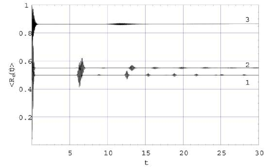
The mean populations of the excited atomic state in the presence of the two modes of coherent state are plotted in Figs. 1 - 4 for various values of $\langle N_{1}\rangle,$ $\langle N_{2}\rangle$, $\delta$ and $k$. For small values of $\delta$ and $k$ the phenomena of quantum revivals and quantum collapses of the Rabi oscillation appear. They are not as regular as those in one-photon or degenerate two-photon case. It can be seen that the amplitudes of the revival oscillations decrease as a consequence of the cavity damping and detuning. In the case of strong damping, the cavity losses are so large that no collapses or revivals phenomena may appear. As a result of the computer simulations it can be said that the decay time and serene duration time for atomic populations are directly affected by the initial photon numbers in the cavity modes. The serene duration time decreases as $\langle N_{1}\rangle,$ $\langle N_{2}\rangle$ decreases and mean populations manifests the more fluctuating behaviour. For large field intensities the detuning influences both revival amplitudes and serene duration time, as well as quasi-stationary atomic population value.

Since two photons are absorbed and/or emitted by the atom simultaneously in the cavity, one can tell that the behavior of photon numbers of mode 2 shows the exactly same manner as for the mode 1. Therefore in Figs.5 -8 we have plotted the mean photon number for first cavity mode. The mean photon numbers exhibit the same pattern of collapse and revival as the atomic population. A comparison of Figs. 1-8 shows that the photon numbers more significantly affected by cavity damping than the atomic population. In the case of strong damping or detuning the mean photon number decays exponentially.

Perhaps a better appreciation of the statistics can be had by examining second-order correlation function $G^{(2)}$ as a function of time t. The second-order correlation functions for two cavity fields may be defined as

For strictly coherent field $G^{(2)}(0)=0$ whereas negative values of $G^{(2)}$ lead to the antibunching of the field. In dressed-state representation the second-order correlation function becomes

In Figs. 9 and 10 we plot $G_{1}^{(2)}$ for different detuning and damping parameters and large initial field intensities. For undamped resonant cavity collapses and revivals appear. In the case of collapse in the absence of detuning (or cavity damping), $G_{1}^{(2)}\lesssim 0$ , the oscillations show both bunching and antibunching features. In the cases of nonzero damping and detuning the antibunching effects almost disappear. The amplitudes of the revivals oscillations will be damped by small cavity losses to the extent that antibunching appears only at the very beginning of the time evolution. For large detuning the second-order correlation function $G_{1}^{(2)}>0$ for every $t$.

Finally, we study the field and atomic squeezing. In order to investigate the squeezing properties of the radiation field we define the slowly varying Hermitian quadrature operators for fields

The commutation of $X^{(i)}_{1}$ and $X^{(i)}_{2}$ is $[X^{(i)}_{1},X^{(i)}_{2}]=\imath/2$. The variances $(\Delta X^{(i)}_{j})^{2}=\langle(X^{(i)}_{j})^{2}\rangle-\langle X^{(i)}_{j}\rangle^{2}\quad(j=1,2)$ satisfy the uncertainty relation $(\Delta X^{(i)}_{1})^{2}(\Delta X^{(i)}_{2})^{2}\geq 1/16$. For the vacuum and coherent states of the field the variances are equal 1/4. The field is in a squeezed state if there takes place $(\Delta X^{(i)}_{j})^{2}<1/4$ for either $j=1$ or $2$.

The condition for squeezing in the $j$th quadrature $\Delta X^{(i)}_{j}$ can be written simply as

where the squeezing factor is

For the sake of definiteness we study the squeezing properties of the first cavity mode. In terms of the photon operators, one can readily find that the squeezing parameter of the first quadrature component and for the first cavity mode may be written as

where

and $\langle a_{1}^{+}a_{1}\rangle=\langle N_{1}(t)\rangle$.

Values $S(t)<1$ imply squeezing in the first quadrature component. In Figs. 11 and 12 we have plotted $S(t)$ for different values of $k$ and $\delta$ and large input field intensities. For $k=0$ there is some amount of squeezing which appears only at the very beginning of the time and this decreases with increasing of $\delta$ in contrast with degenerate two-photon JCM. But this model does not give rise to significant squeezing. For nonideal cavity the effect is vanished. So, the cavity damping is seen to have an appreciable effect on the squeezing properties.

To investigate atomic squeezing we introduce the dispersive and absorptive components of slowly varying atomic dipole moment 32 32

and

respectively. They obey the commutation relation

and the corresponding uncertainty relation

The atomic state is said to be squeezed when $\sigma_{1}$ or $\sigma_{2}$ satisfies the relation

Since

the condition described by Eq. (9) can be rewritten as

or

for squeezing in the dispersive or absorptive component of the dipole moment.

Here

and $\langle\sigma_{3}\rangle=\langle R_{e}\rangle-\langle R_{g}\rangle$ is atomic inversion in terms of dressed states representation.

The results for the squeezing parameters for different values of $k$ and $\delta$ and moderate input intensities ($\langle n_{1}\rangle=15,\langle n_{2}\rangle=10)$ have been shown on Figs. 13-16. The dispersive component $F_{1}$ does not squeeze at the very beginning of the time, the absorptive component $F_{2}$, on the other hand, goes below 1 with virtually no time delay.

Both $F_{1}$ and $F_{2}$ shows squeezing recurrently only for small times of the atom-field interaction. As that has been mentioned earlier 23 23 that squeezing does not show up in either case until after $\langle N_{i}\rangle\geq 7.0$. The amount of squeezing decreases with increase of damping parameter $k$. If the parameter $k$ is large enough the squeezing in dispersive component vanishes and the squeezing in absorptive component of dipole moment undergoing only one squeezing minimum. For high input intensities (not shown in Graphs) the influence of damping parameter on squeezing amount is more dramatic than one for medium input intensities. And with increasing the detuning parameter $\delta$ the amount of squeezing in dispersive and absorptive component also decreases while the time interval, for which the squeezing appears, increases.

In this paper we have investigated the nondegenerate two-photon Jaynes-Cummings model with damping and detuning. We have set kinetic equations for density matrix of the considered system in secular approximation and with using the dressed-state representation. These equations are solved numerically for different detuning of atomic levels and damping parameter. On the basis of these equation the analysis of the dynamical behaviour of mean values of atomic populations, mean photon numbers, field coherence and squeezing has been carried out. The effects of cavity damping will significantly attenuate the amplitudes of mean atomic populations, mean photon number revivals. The revivals of the second-order photon correlation function will be damped by small cavity losses to the extent than antibunching appears only at the very beginning of the time. Cavity damping has an appreciable effect on the squeezing properties of fields and atomic dipole moment. For moderate damping parameter the field squeezing is vanished and the amount of atomic squeezing sharply decreases. In this paper we shall restrict our consideration to the coherent input for fields and ignore the Stark shift. A further discussion on dissipative NTPJCM including the consideration of initial squeezed and thermal states for cavity fields and Stark shift is planned to be reported in the subsequent paper.

References

• (1) W. Walter, Usp. Fiz. Nauk. 166, 777 (1996).
• (2) S.M. Barnett and P.L. Knight, Phys.Rev. A 33, 2444 (1986).
• (3) R.R. Puri and G.S. Agarwal, Phys.Rev. A 35, 3433 (1987).
• (4) E.K. Bashkirov, Fam Le Kien and A.S. Shumovsky, Physica A 167 (1990). V.167.
• (5) H.-J. Briegel, B.-G. Englert, Phys.Rev. A 47, 3311 (1993).
• (6) A.J. Wonderen, Phys. Rev. A 56, 3116 (1997).
• (7) C.K. Law, T.W. Chen and Leung, Phys.Rev. A 61, 0238008 (2000).
• (8) A. Linder A. et al., Eur. Phys. J. D 17, 99 (2001).
• (9) J. Eiselt and H. Risken, Opt.Commun. 72, 351 (1989).
• (10) J. Gea-Banachloce, Phys. Rev. A 47, 2221 (1993).
• (11) B.G. Englert, M. Naraschevski and D. Schenzlr, Phys. Rev. A 50 2667 (1994).??????
• (12) L.-M. Kuang, X. Chen, G.-H. Chen and M.-L. Ge, Phys. Rev. A 56, 3139 (1997).
• (13) H.A. Hessian and H.J. Ritsch, J.Phys. B 35, 4619 (2002).
• (14) M. Brune, J.M. Raimond, P.Goy, L. Davidovich and S. Haroche, Phys. Rev. Let. 59 1899 (1987).
• (15) R.R. Puri and G.S. Agarwal, Phys.Rev. A 39, 3879 (1988).
• (16) G. Adam, J. Seke and O. Hittmair, Phys. Rev. A 42, 5522 (1990).
• (17) M.Y. Hamza and S.J. Qamar, J.Opt. B 2, 323 (2000).
• (18) L. Zhou, H.S. Song, Y.X. Luo and C. Li, Phys. Lett. A 284 , 156 (2001).
• (19) L. Zhou L., H.S. Song, C.Li and Y.Q. Guo, Chinese Physics 12, 45 (2003).
• (20) S.-C. Gou, Phys. Rev. A 40 5116 (1989); 40, 4097 (1991).
• (21) C.C. Gerry and J.H. Eberly, Phys. Rev. A 42, 6805 (1990).
• (22) A. Joshi and R.R. Puri, Phys. Rev. A 42, 4336 (1990).
• (23) C.C. Gerry and R.F. Welch, J.Opt.Soc.Am. B 9, 290 (1992).
• (24) M.M. Ashraf and M.S.K. Razmi, Phys. Rev. A 45, 8121 (1992).
• (25) A.M. Abdel-Hafez, Phys. Rev. A 45, 6610 (1992).
• (26) M.M. Ashraf, Phys.Rev. A. 50, 5116 (1994).
• (27) H. Iwasawa and K. Matsuo K., Optics Commun. 117, 550 (1995).
• (28) A.-S.F. Obada, A.M. Abdel-Hafez and H.A. Hessian, Intern. J. Theor. Phys. 39, 1499 (2000).
• (29) M. Abdel-Aty, S. Abdel-Khalek and A.-S.F. Obada, Chaos, Solit. Fractals 12, 2015 (2001).
• (30) R.H. Xie and V.H. Smith Jr., Physica A 307, 207 (2002).
• (31) J. Aliaga and J.L. Gruver, Phys.Lett. A 221, 19 (1996).
• (32) S. Mahmood and M.M. Ashraf, Opt. Commun. 33, 355 (1996).
• (33) N.B. Narozhny, J.J. Sanchez-Mondragon and J.H. Eberly, Phys.Rev. A 23, 236 (1981).
V Appendix
Refer to caption
Figure 1: Atomic population of an excited level for ⟨N1⟩=⟨N2⟩=5,δ=10\langle N_{1}\rangle=\langle N_{2}\rangle=5,\,\delta=10 and 1. k=0k=0, 2. k=0.001k=0.001, 3. k=0.01k=0.01.   Curve 3 corresponds to value ⟨Re​(t)⟩−0.1\langle R_{e}(t)\rangle-0.1
Figure 2: Atomic population of an excited level for ⟨N1⟩=⟨N2⟩=5,δ=10\langle N_{1}\rangle=\langle N_{2}\rangle=5,\,\delta=10 and 1. k=0k=0, 2. k=0.001k=0.001, 3. k=0.01k=0.01. Curve 1 corresponds to value ⟨Re​(t)⟩+0.2\langle R_{e}(t)\rangle+0.2, and curve 3 corresponds to ⟨Re​(t)⟩−0.2\langle R_{e}(t)\rangle-0.2
Figure 3: Atomic population of an excited level for ⟨N1⟩=⟨N2⟩=30,k=0.001\langle N_{1}\rangle=\langle N_{2}\rangle=30,\,k=0.001 and 1. δ=0\delta=0;   2. δ=20\delta=20; 3. δ=100\delta=100.
Figure 4: Atomic population of an excited level for ⟨N1⟩=⟨N2⟩=30,δ=10\langle N_{1}\rangle=\langle N_{2}\rangle=30,\,\delta=10 and 1. k=0k=0;   2. k=0.0001k=0.0001;  3. k=0.001k=0.001; 4. k=0.01k=0.01. Curve 1 corresponds to value ⟨Re​(t)⟩−0.2\langle R_{e}(t)\rangle-0.2, curve 3 corresponds to ⟨Re​(t)⟩+0.2\langle R_{e}(t)\rangle+0.2, curve 4 corresponds to ⟨Re​(t)⟩+0.4\langle\ R_{e}(t)\rangle+0.4.
Figure 5: Mean photon number in the first field mode for ⟨N1⟩=⟨N2⟩=5,k=0.001\langle N_{1}\rangle=\langle N_{2}\rangle=5,\,k=0.001 and 1. δ=0\delta=0; 2. δ=10\delta=10; 3. δ=100\delta=100.
Figure 6: Mean photon number in the first field mode for ⟨N1⟩=⟨N2⟩=5,δ=10\langle N_{1}\rangle=\langle N_{2}\rangle=5,\,\delta=10 and 1. k=0k=0, 2. k=0.001k=0.001, 3. k=0.01k=0.01.
Figure 7: Mean photon number in the first field mode for ⟨N1⟩=⟨N2⟩=30,k=0.001\langle N_{1}\rangle=\langle N_{2}\rangle=30,\,k=0.001 and 1. δ=0\delta=0;   2. δ=20\delta=20;  3. δ=100\delta=100.
Figure 8: Mean photon number in the first field mode for ⟨N1⟩=⟨N2⟩=30,δ=10\langle N_{1}\rangle=\langle N_{2}\rangle=30,\,\delta=10 and 1. k=0k=0;   2. k=0.0001k=0.0001;  3. k=0.001k=0.001; 4. k=0.01k=0.01.
Figure 9: Second order correlation function for the first field mode for ⟨N1⟩=⟨N2⟩=30,k=0.001\langle N_{1}\rangle=\langle N_{2}\rangle=30,\,k=0.001 and 1. δ=0\delta=0;   2. δ=10\delta=10;    3. δ=20\delta=20;  4. δ=100\delta=100.
Figure 10: Second order correlation function for the first field mode for ⟨N1⟩=⟨N2⟩=30,δ=10\langle N_{1}\rangle=\langle N_{2}\rangle=30,\,\delta=10 and 1. k=0k=0;   2. k=0.001k=0.001;  3. k=0.01k=0.01.
Figure 11: Squeezing in the first field mode for ⟨N1⟩=⟨N2⟩=50,k=0\langle N_{1}\rangle=\langle N_{2}\rangle=50,k=0 and 1.  δ=10\delta=10; 2.  δ=100\delta=100.
Figure 12: Squeezing in the first field mode for ⟨N1⟩=⟨N2⟩=50,δ=10\langle N_{1}\rangle=\langle N_{2}\rangle=50,\,\delta=10 and 1. k=0k=0; 2. k=0.0001.k=0.0001.
Figure 13: Atomic dipole moment dispersive component for ⟨N1⟩=15,\langle N_{1}\rangle=15,\, ⟨N2⟩=10,\langle N_{2}\rangle=10,   k=0.001k=0.001 and  1.  δ=50\delta=50 ; 2. δ=100\delta=100.
Figure 14: Atomic dipole moment absorptive component for ⟨N1⟩=15,\langle N_{1}\rangle=15,\, ⟨N2⟩=10,\langle N_{2}\rangle=10,   k=0.001k=0.001 and  1.  δ=50\delta=50;  2. δ=100\delta=100.
Figure 15: Atomic dipole moment dispersive component for ⟨N1⟩=15,\langle N_{1}\rangle=15,\, ⟨N2⟩=10,\langle N_{2}\rangle=10,   δ=10\delta=10 and  1.  k=0.001k=0.001;  2. k=0.01k=0.01.
Figure 16: Atomic dipole moment absorptive component for ⟨N1⟩=15,\langle N_{1}\rangle=15,\, ⟨N2⟩=10,\langle N_{2}\rangle=10,  δ=10\delta=10 and  1.  k=0.001k=0.001;  2. k=0.01k=0.01.