Few-body spin couplings and their implications for universal quantum computation
Abstract
Electron spins in semiconductor quantum dots are promising candidates for the experimental realization of solid-state qubits. We analyze the dynamics of a system of three qubits arranged in a linear geometry and a system of four qubits arranged in a square geometry. Calculations are performed for several quantum dot confining potentials. In the three-qubit case, three-body effects are identified that have an important quantitative influence upon quantum computation. In the four-qubit case, the full Hamiltonian is found to include both three-body and four-body interactions that significantly influence the dynamics in physically relevant parameter regimes. We consider the implications of these results for the encoded universality paradigm applied to the four-electron qubit code; in particular, we consider what is required to circumvent the four-body effects in an encoded system (four spins per encoded qubit) by the appropriate tuning of experimental parameters.
pacs
03.67.Pp, 03.67.Lx, 75.10.JmI Introduction
Electron spins in semiconductor quantum dots are a leading candidate for the physical realization of qubits in a quantum computer LossDiVincenzo98. Although any quantum algorithm can be implemented using single-qubit and two-qubit gates MAN/ILC, many such algorithms realize substantial increases in efficiency by exploiting simultaneous interactions among three or more qubits D. Bacon, J. Kempe, D.A. Lidar and K.B. Whaley 2000; J. Kempe, D. Bacon, D.A. Lidar, and K.B. Whaley 2001; D.P. DiVincenzo, D. Bacon, J. Kempe, G. Burkard, and K.B. Whaley 2000; D.A. Lidar and L.-A. Wu 2002; D. Bacon, J. Kempe, D.P. DiVincenzo, D.A. Lidar, and K.B. Whaley 2001; M.H. Freedman 2003; R. Raussendorf and H.J. Briegel 2001; D.A. Lidar, D. Bacon, J. Kempe, and K.B. Whaley 2001; A.M. Steane 1999; Preskill; Gottesman 1997; P.W. Shor 1996; E. Farhi, J. Goldstone, S. Gutmann, J. Lapan, A. Lundgren, D. Preda 2001; D. Bacon, K.R. Brown, K.B. Whaley 2001. In order to employ such simultaneous interactions, it is essential to understand in detail the many-body dynamics of the system of coupled qubits. More generally, since a practical quantum computer may need to contain as many as qubits Preskill, it is essential to characterize the effect of many-body interactions on the system’s overall energy landscape.
In past work MizelLidar; MizelLidarB, we used a model confining potential of superposed parabolic minima to demonstrate that three-body effects significantly influence the Hamiltonian of three electrons confined to three quantum dots at the vertices of an equilateral triangle and that four-body effects are significant for four electrons confined to a tetrahedral arrangement of four dots. Here we extend these results in two ways. First, we analyze three quantum dots in a linear geometry 3inaline_figure and four dots in a square geometry G. Burkard, H.-A. Engel and D. Loss 2000 since these geometries are more likely to occur in a real quantum computer apparatus. Second, by employing a Gaussian shape for the confining potential of each well Hu:99, we explore the sensitivity of the many-body effects to the form of the confining potential. In both cases, a non-perturbative calculation finds that many-body effects contribute appreciably to the Hamiltonian. We note that Scarola et al. V.W. Scarola, K. Park, and S. Das Sarma 2004; V.W. Scarola and S. Das Sarma 2005 have demonstrated that the application of a magnetic field allows chiral terms to arise in the spin Hamiltonian, which modifies this Hamiltonian in another important manner as compared to the naive Heisenberg form.
To date, discussions of quantum dot quantum computation have nearly always assumed pairwise Heisenberg interactions. In view of the above result, this implies that computational errors may occur in the context of quantum computers using electron spin qubits in quantum dots, unless one always simultaneously couples only disjoint pairs of dots. There are at least four circumstances where this may be undesirable or even infeasible. One is fault tolerant quantum error correction, where simultaneous operations on several coupled dots have been associated with better error thresholds. A second is adiabatic quantum computation E. Farhi, J. Goldstone, S. Gutmann, J. Lapan, A. Lundgren, D. Preda 2001, in which the final Hamiltonian may include the simultaneous interactions that we discuss here. We will not analyze these possibilities here, although we believe that the methods we discuss below are relevant to them.
We will focus on two other contexts, that of “encoded universality” (EU) D. Bacon, J. Kempe, D.A. Lidar and K.B. Whaley 2000; J. Kempe, D. Bacon, D.A. Lidar, and K.B. Whaley 2001; D.P. DiVincenzo, D. Bacon, J. Kempe, G. Burkard, and K.B. Whaley 2000; D. Bacon, J. Kempe, D.P. DiVincenzo, D.A. Lidar, and K.B. Whaley 2001; D.A. Lidar and L.-A. Wu 2002 and that of computation on decoherence-free subspaces (DFSs) D. Bacon, J. Kempe, D.A. Lidar and K.B. Whaley 2000; J. Kempe, D. Bacon, D.A. Lidar, and K.B. Whaley 2001; Zanardi 1999 and supercoherent qubits D. Bacon, K.R. Brown, K.B. Whaley 2001. In these cases, the goal is to perform universal quantum computation using (EU:) only the most easily controllable interaction, or (DFS, supercoherence:) using only interactions that preserve the code subspace, since that subspace offers protection against certain types of decoherence. (Strong and fast exchange interaction pulses can further be used to suppress decoherence L.-A. Wu and D.A. Lidar 2002 and to eliminate decoherence-induced leakage L.-A. Wu, M.S. Byrd, D.A. Lidar 2002.)
We will refer to these cases collectively as “encoded quantum computation.” It turns out that universal quantum computation using only the Heisenberg exchange interaction is an extremely attractive possibility in encoded models, and we will consider it in detail below. After establishing that four-body interaction terms can arise in a Heisenberg exchange Hamiltonian, we investigate the question of neutralizing their effect by using encoded qubits P. Zanardi and M. Rasetti 1997; D. Bacon, J. Kempe, D.A. Lidar and K.B. Whaley 2000; J. Kempe, D. Bacon, D.A. Lidar, and K.B. Whaley 2001; D. Bacon, J. Kempe, D.P. DiVincenzo, D.A. Lidar, and K.B. Whaley 2001; D.A. Lidar and L.-A. Wu 2002; Zanardi 1999; L.-A. Wu and D.A. Lidar 2002; L.-A. Wu, M.S. Byrd, D.A. Lidar 2002; D.A. Lidar, D. Bacon, J. Kempe and K.B. Whaley 2000; D. Bacon, K.R. Brown, K.B. Whaley 2001; D.A. Lidar, K.B. Whaley 2003. By generalizing the work of Bacon D.M. Bacon 2001, who showed that universal quantum computation was possible using encoded gates with two-body coupling Hamiltonians (i.e., assuming that the Heisenberg Hamiltonian was applicable even when coupling three or more dots at a time), we enumerate tuning conditions on experimental parameters that are needed for the four-body effects to cancel out. An alternative is to design these encoded gates while allowing only pairs of electrons to couple at any given time. This is indeed possible, as shown in Ref. M. Hsieh, J. Kempe, S. Myrgren, K.B. Whaley 2004, for the price of significantly longer pulse sequences per given encoded gate. Nevertheless, in view of the findings reported here and in Refs. V.W. Scarola, K. Park, and S. Das Sarma 2004; V.W. Scarola and S. Das Sarma 2005, this price may be worth paying.
II Three-Electron Case
A system of three electrons within a confining scalar potential obeys the Hamiltonian
| (1) | |||||
| (2) |
in the absence of spin-orbit coupling and external magnetic fields. Although Ref. MizelLidar succeeded in demonstrating significant three-body and four-body effects in systems containing three or more electrons, a confining potential with quadratic minima has certain other characteristics which are unlikely to describe an experimental arrangement; for example, it diverges at large distances from the origin, and the single adjustable parameter forces us to specify very narrow minima whenever we want a high barrier between them. We therefore begin with the Gaussian form
| (3) |
which has two tunable parameters. The three fixed points are collinear and separated by a distance : , , and .
We assume a Heitler-London approximation HL, wherein excited orbital states and states with double occupation of any single dot are neglected (see Ref. V.W. Scarola and S. Das Sarma 2005 for a recent discussion of the validity of this approximation in the context of electron spin qubits). The system’s only degrees of freedom are therefore the spins of the confined electrons, leading to a total of “computational” basis states
| (4) |
In the above, are the three localized orbital ground states; denote the corresponding spin states; is the set of all permutations of ; and is 1 (-1) for even (odd) permutations. For instance, one of the eight (unnormalized) basis states is
To characterize the localized orbital state for each dot, we expand (3) to quadratic order and solve the Schrödinger equation as though the other potential wells were absent:
| (5) |
Unless is small compared to , of course, this is a much coarser approximation than it would be for purely quadratic minima, so we refine it by centering and at the points which minimize and . Because these orbitals overlap at least slightly for any finite , the states (4) are not orthogonal.
We now define to be the matrix representation of in the basis (4), and expand it in terms of tensor products of Pauli matrices:
This expansion is always possible, since the set of -fold tensor products of Pauli matrices constitutes a complete orthonormal basis for the linear vector space of all matrices. Because we have written the basis (4) in the form , these Pauli matrices can be associated with spin operators on each of the three quantum dots. For example, we can write , where the notation means the Pauli operator applied to the electron in the quantum dot at , and where is the identity matrix. (We exclude from the definition of the matrices ; thus, the have the dimensions of energy.) In the case of an arbitrary matrix, 64 complex numbers would be required to specify our , but the operator (1) clearly has certain properties which constrain the values of the coefficients, such as Hermiticity, reflection symmetry, rotation symmetry, inversion symmetry, and invariance under permutation of the electrons’ labels. Once these symmetries have been accounted for, the may be characterized by just three real quantities:
| (6) |
where , and is the pairwise coupling coefficient between the spins of the electrons in dots and . Here and elsewhere, we use symmetry considerations to reduce the number of coupling coefficients in our equations; in this case, the reflection symmetry of (3) through the - plane implies that . Physically, the constant quantifies the coupling between adjacent spins, while describes the coupling between the spins at opposite ends of the row.
Defining , one finds that
| (7) |
where
| (8) | |||||
The expansion (7) reveals that any simultaneous eigenstate of and is also an eigenstate of . We can construct such simultaneous eigenstates by using the Clebsch-Gordan table twice, first to combine the spin of the electron in dot with the spin of the electron in dot , and then to combine that spin-1 (or spin-0) system with the spin of the electron in dot :
| (9) | |||||
where the indices on the left-hand side denote the values of , , and respectively. Although the states are not orthonormal, the eight states (9) are orthogonal, and they are also eigenvectors of the matrix (7), which means that has been diagonalized. To obtain the parameters , we will choose three eigenstates with different good quantum numbers, and observe that their energies can be evaluated either by matrix algebra or by integrating microscopically over the axes and the spins to compute the expectation value of (1):
| (10) |
Inserting (7) into the left-hand side, for three distinct combinations of the good quantum numbers , yields
| (11) | |||||
while the corresponding wave functions (9) turn the right-hand side into
| (12) | |||||
The evaluation of these matrix elements and overlap integrals is a tedious, but straightforward procedure given the microscopic forms of and in (1), (3), and (5). Combining Eqs. (8), (11), and (12), we thus compute , , and in terms of and the dimensionless system parameters
| (13) | |||||
| (14) | |||||
| (15) |
Physically, the quantity is the ratio of the height of the potential barrier between wells to the energy of the orbital ground state (5), while is the ratio of the equilibrium Coulomb repulsion potential to the energy of the orbital ground state, and is the ratio of the individual well depth to the ground state energy.
Here and in the following section, we have estimated experimentally relevant values of and as is done in Ref. LossDiVincenzo98. We assume that the width of the function (5), which is , must be roughly equal to the separation between adjacent dots ; using (13), we conclude that 1. For GaAs heterostructure single dots, 13, 0.067 , and 3 meV, which according to (14) means that 1.5.
A potential of the form (3) is most suitable for quantum computation when is close to 1; if the inverted Gaussian decays too quickly in space, the spin coupling in the system becomes negligible, and if it decays too slowly, the local minima in tend to coalesce at the center. Using 1 meV, 3 meV LossDiVincenzo98, and our prior estimate of 1.5, we obtain the relation , by applying (13), (14), and (15). Noting that the parameter has very little influence on any of the coupling constants over physically realistic ranges of and (and in any event depends on quantities, such as , which are difficult to tune experimentally), we henceforth set .
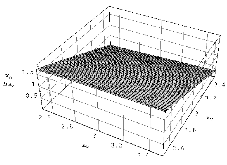
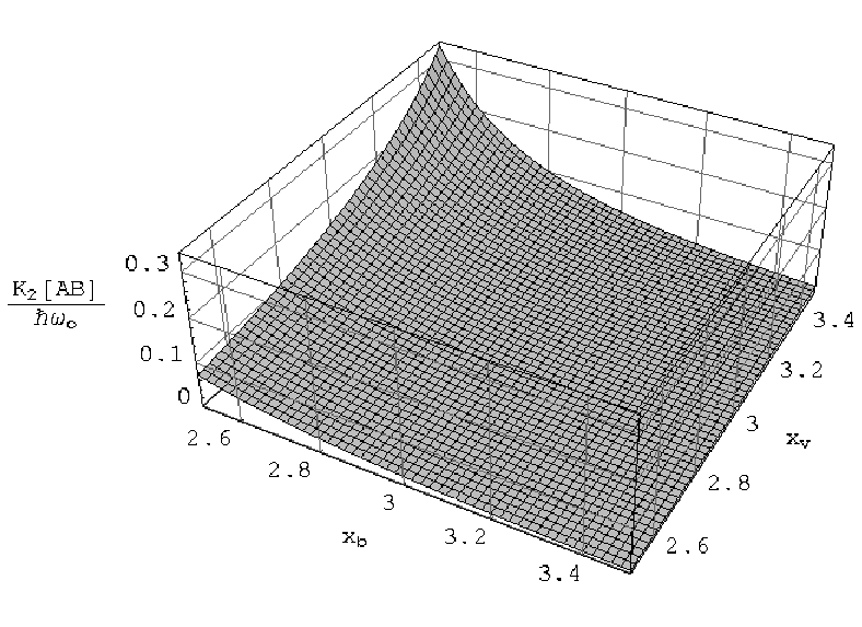
Fig. 1 shows the energy shift as a function of the system parameters . As one might expect, this spin-independent quantity increases with increasing and decreasing (whenever decreases, there is greater orbital overlap and thus more Coulomb repulsion, irrespective of spin state). The coupling constants and are plotted in Fig. 2 and Fig. 3 respectively. We notice that they differ (which rules out the simple Heisenberg form ), and that is only about an order of magnitude smaller than , as we have confirmed by studying and on a logarithmic scale. In the context of quantum computation, this demonstrates that a nearest-neighbor approximation for the coupling between dots is insufficient (see also Ref. V.W. Scarola and S. Das Sarma 2005, where a similar conclusion was reported using a low-energy Hubbard model with one electron per site).
III Four-Electron Case
For the case of four quantum dots arranged in a square of side , our formalism is more complex in detail but identical in structure. We therefore describe the computation only in outline.
The confining potential in the coordinate Hamiltonian
| (16) |
now becomes
where , , , and . Our computational basis consists of 16 fully antisymmetrized vectors of the form
| (17) | |||||
The form of remains the same; to maintain the required geometrical symmetries, we now shift all four localized orbital wave functions an equal distance toward the point .
Expanding in terms of products of Pauli matrices,
we discover by applying the symmetries of (16) that four-body terms now appear with nonzero coupling coefficients:
| (18) | |||||
where is the four-body coupling coefficient among the spins of the electrons in dots , , , and . Physically, the constant describes the pairwise coupling between adjacent spins, while describes the pairwise coupling between non-adjacent spins, describes four-body interactions concentrating on pairs of adjacent spins, and describes four-body interactions concentrating on pairs of non-adjacent spins. We define , which leads us to
| (19) | |||||
where
| (20) | |||||
Applying the Clebsch-Gordan table three times creates sixteen simultaneous eigenstates of , , and . Inserting five of these states with different quantum numbers into (10) yields five equations for the five unknowns in terms of the eigenstate energies. As before, these energies may be expressed in closed form as functions of , , and by integrating the right-hand side of (10) explicitly.
The energy shift for the square case is plotted in Fig. 4; as before, this constant is largest for strongly Coulomb-coupled dots separated by low potential barriers. Figs. 5, 6, 7, and 8 depict the coupling coefficients , , , and respectively. The departure from the pairwise Heisenberg picture is even more pronounced here: we see that for physically relevant values of the parameters , the four-body coefficient is of the same order of magnitude as the two-body coefficient , while 0.1, as is confirmed by plotting , , , and on a logarithmic scale.. Typically, is opposite in sign to , leading to a particularly important competition between the two-body and four-body interactions.
In order to confirm that the qualitative similarities between our final results and those of Ref. MizelLidar were not artifacts of having made two broad changes to rather than one, we also analyzed both the and dot geometries using a confining potential of superposed quadratic minima. The variation of the coupling coefficients, within experimentally relevant ranges of and (analogous to Figs. 1 through 8), strongly resembled that for the Gaussian potential in all cases.
IV Computing in the Presence of Four-Body Interactions Using Encoded Qubits
We have shown that coupling three dots simultaneously quantitatively modifies the value of the exchange constant, and that coupling four dots simultaneously switches on a four-body interaction term of the form and its permutations. This conclusion appears to be robust under changes in dot geometry and in the confining potential. A natural question is whether there exist methods to cancel the four-body correction. The issue is particularly urgent when one considers encoded quantum computation (EQC). In many known constructions of universal gates for EQC P. Zanardi and M. Rasetti 1997; D. Bacon, J. Kempe, D.A. Lidar and K.B. Whaley 2000; D.P. DiVincenzo, D. Bacon, J. Kempe, G. Burkard, and K.B. Whaley 2000; J. Kempe, D. Bacon, D.A. Lidar, and K.B. Whaley 2001; D. Bacon, J. Kempe, D.P. DiVincenzo, D.A. Lidar, and K.B. Whaley 2001; D.A. Lidar and L.-A. Wu 2002; Zanardi 1999; L.-A. Wu and D.A. Lidar 2002; L.-A. Wu, M.S. Byrd, D.A. Lidar 2002; D.A. Lidar, D. Bacon, J. Kempe and K.B. Whaley 2000; D. Bacon, K.R. Brown, K.B. Whaley 2001; D.A. Lidar, K.B. Whaley 2003; M. Hsieh, J. Kempe, S. Myrgren, K.B. Whaley 2004, there arises the need to simultaneously couple several spins. One of the most popular codes, described in detail below, uses four spins per encoded, or logical qubit P. Zanardi and M. Rasetti 1997; D. Bacon, J. Kempe, D.A. Lidar and K.B. Whaley 2000; J. Kempe, D. Bacon, D.A. Lidar, and K.B. Whaley 2001; D. Bacon, J. Kempe, D.P. DiVincenzo, D.A. Lidar, and K.B. Whaley 2001; D.A. Lidar and L.-A. Wu 2002; Zanardi 1999; L.-A. Wu and D.A. Lidar 2002; L.-A. Wu, M.S. Byrd, D.A. Lidar 2002; D.A. Lidar, D. Bacon, J. Kempe and K.B. Whaley 2000; D. Bacon, K.R. Brown, K.B. Whaley 2001; D.A. Lidar, K.B. Whaley 2003. For this code, universal computation requires that four spins be coupled at the same time using pairwise Heisenberg interactions. Hence a priori it appears that EQC using the four-qubit code suffers from a fundamental flaw. We now explore whether the four-qubit code may be implemented in such a way that each four-body coupling is either cancelled or reduced to an overall phase. Our findings highlight problems that the four-body terms present in the context of EQC, and also provide an interesting perspective on how the four-body terms may need to be dealt with in general.
IV.1 The Code
Let us descibe the four-spin DFS code, first proposed in Ref. P. Zanardi and M. Rasetti 1997 in the context of providing immunity against collective decoherence processes (see Ref. D.A. Lidar, K.B. Whaley 2003 for a review). Let the singlet and triplet states of two electrons be denoted as
Then a single encoded DFS qubit is formed by the two singlets of four spins, i.e., the two states with zero total spin . These states are formed by combining two singlets of two pairs of spins (), or triplets of two pairs of spins, with appropriate Clebsch-Gordan coefficients ():
| (21) | |||||
| (22) | |||||
| (23) | |||||
As shown in Refs. D. Bacon, J. Kempe, D.A. Lidar and K.B. Whaley 2000; J. Kempe, D. Bacon, D.A. Lidar, and K.B. Whaley 2001, the Heisenberg interaction can be used all by itself to implement universal quantum computation on this type of code. The Heisenberg interaction is closely related to the exchange operator , defined as
| (24) |
via . The difference in their action as gates is only a phase, so that we will use and interchangeably from now on and write . The have a simple action on the electronic spin up/down states, as seen from the matrix representation (24): the states and are invariant, whereas and are exchanged. Using this, it is simple to show that, in the basis, the exchange operators can be written as D.A. Lidar, D. Bacon, J. Kempe and K.B. Whaley 2000; J. Kempe, D. Bacon, D.A. Lidar, and K.B. Whaley 2001
where are the encoded Pauli matrices , i.e., the Pauli matrices acting on the states. It follows from the Euler angle formula, (a rotation by angle about the axis , given in terms of three successive rotations about the and axes), that one can perform all single encoded-qubit operations on the DFS states, simply by switching the exchange interaction on and off. Note that the Euler angle formula is satisfied by any pair of non-parallel axes, but orthogonal axes may be more convenient. One can obtain an encoded operation by switching on two interactions simultaneously for the appropriate time intervals:
Use of the Euler angle formula requires a Hamiltonian which is a sum of exchange terms with controllable coefficients :
This is achievable, e.g., by using local magnetic fields LossDiVincenzo98; G. Burkard, D. Loss and D.P. DiVincenzo 1999; G. Burkard, H.-A. Engel and D. Loss 2000; Hu:99; X. Hu and S. Das Sarma 2001, by ferroelectric gates J. Levy 2002a, or by optical rectification J. Levy 2002b. It is important to emphasize that the last two methods J. Levy 2002a; J. Levy 2002b do not require magnetic field control, hence overcome at least in part the problems with EQC raised in Refs. V.W. Scarola, K. Park, and S. Das Sarma 2004; V.W. Scarola and S. Das Sarma 2005. This is an important advantage with regards to EQC, which renders these electrical-only type control methods distinctly preferable to those using magnetic fields. However, residual magnetic fields, e.g., due to nuclear spin impurities, do remain a problem, especially in the group III-V semiconductors, such as GaAs R. de Sousa and S. Das Sarma 2003. In silicon-based architectures this problem can be minimized by isotopic purification E. Yablonovitch, H.W. Jiang, H. Kosaka, H.D. Robinson, D.S. Rao, and T. Szkopek 2003.
IV.2 Effect of the Four-Body Terms on a Single Encoded Qubit
Let us now consider how the four-body terms act on the DFS code. Using the results above, we find that
where is the identity operator. Also,
and similarly . Thus all fourth-order terms as long we restrict their action to the subspace encoding one qubit. This implies that the encoding into the 4-qubit DFS is immune to the fourth-order terms. In other words, when this encoding is used, the problem of the computational errors induced by the undesired fourth-order terms simply disappears, as long as we restrict our attention to a single encoded qubit.
IV.3 Two Encoded Qubits
We must also be able to couple encoded qubits via a non-trivial gate such as controlled-phase:. This is one way to satisfy the requirements for universal quantum computation A. Barenco, C.H. Bennett, R. Cleve, D.P. DiVincenzo, N. Margolus, P. Shor, T. Sleator, J. Smolin and H. Weinfurter 1995, though it is also possible to complete the set of single-qubit gates by measurements E. Knill, R. Laflamme, and G. J. Milburn 2001. Two encoded qubits of the form (22), (23) occupy a four-dimensional subspace of the zero total spin subspace of spins. The zero total spin subspace is -dimensional. A very useful graphical way of seeing this, introduced in Ref. J. Kempe, D. Bacon, D.A. Lidar, and K.B. Whaley 2001 but also known as a Bratteli diagram, is depicted in Fig. 9.
As more spins are added (horizontal axis), there are more possibilities for constructing a state with given total spin (vertical axis). In the case of four spins there are two paths leading from the origin to ; these correspond exactly to the and code states. For eight spins there are such paths. Only four of these correspond to the four basis states . It is convenient to label paths according to the intermediate total spin: the state , where is the total spin of spin-1/2 particles, uniquely corresponds to a path in Fig. 9 (we omit the origin in this notation), and the form a complete set of commuting observables J. Kempe, D. Bacon, D.A. Lidar, and K.B. Whaley 2001. E.g.,
On the right we have indicated the path in Fig. 9 corresponding to each state. The other states with zero total spin can be similarly described. Thus the set of states forms a basis for the subspace of zero total spin of spin-1/2 particles. Henceforth we will find it convenient to represent exchange operators in this basis. We will order the basis states as follows: first the four code states as above, then
E.g., in this basis the operator has the representation11 1 All matrix calculations reported here were performed with Mathematica.
Recall that the first four rows refer to the code space. It is then clear that mixes the code space with four of the remaining ten states that have zero total spin. This is a general feature of all exchange operators acting on two code blocks simultaneously. For this reason it is impossible to couple two code blocks in one step, while preserving the code space.
IV.4 Enacting an Encoded Controlled-Phase Gate
For the 4-qubit code above, procedures implementing a gate were first given in Refs. D. Bacon, J. Kempe, D.A. Lidar and K.B. Whaley 2000; J. Kempe, D. Bacon, D.A. Lidar, and K.B. Whaley 2001. Recently, Bacon (D.M. Bacon 2001, App. E) found a simplified scheme which is a useful starting point for our purposes. Bacon’s implementation of a gate between two pairs of 4-qubit blocks (qubits - and qubits -) involves a sequence of elementary gates, each of which requires that several simultaneous exchange interactions be switched on and off. We will here take the approach of utilizing Bacon’s construction, while making some modifications due to the appearance of three- and four-body corrections. For ease of visualization, we will assume that the two blocks are squares of side and that dots and are separated by a distance , although nearly all of the following calculations are independent of the exact spatial relationship between the blocks.
The gates are (adapting the notation of (D.M. Bacon 2001, App. E))
where
In terms of these gates, the controlled-phase gate can be written as
where can be executed in one step since by inspection the two gates operate on the two blocks separately (and identically). This gate sequence operates in the entire -dimensional subspace of states of spins: the code space is left after application of , but is returned to at the end of the sequence, when is applied. Hence our single-qubit considerations above do not apply: even if a four-body interaction acts as the identity operator on a single encoded qubit, it may act non-trivially in the larger space. We must therefore carefully analyze the action of this gate sequence in light of the three- and four-body corrections.
The key point in Bacon’s construction of the gate sequence is to ensure that each gate acts “classically,” i.e., it only couples a given basis state to another, without creating superpositions of such basis states (that the gates above act in this manner is not at all simple to see directly, but is the reason for the particular choice of angles in the gates). Here we will show that, in order to still satisfy this key point, it is necessary to tune the four-body exchange coupling constants. Thus, to enact a gate in the presence of four-body interactions, there needs to be sufficient flexibility in tuning the four-body coupling. We note that there are other ways to obtain a gate M. Hsieh, J. Kempe, S. Myrgren, K.B. Whaley 2004; our point here is mostly to explore the implications of the four-body terms in a context of some general interest. Let us now consider each of the gates in detail, in increasing order of complexity.
IV.4.1 The Gate
only involves a single exchange interaction, and so is unmodified in the presence of the three- and four-body corrections:
where and .
IV.4.2 The Gate
involves dots , , and , with dots and simultaneously coupled to , and hence experiences a three-body correction to the exchange constants. In addition, a coupling between dot and dot will arise, which forces our modified gate to have the form
where
It is seen that this gate operates “classically,” and is non-diagonal, only when is either or chosen such that is an even integer. In both cases, we recover Bacon’s functional form:
IV.4.3 The Gate
Bacon’s gate is
involves coupling between four dots, so experiences both quantitative three-body corrections and a four-body qualitative correction. Since the four spins in are coupled symmetrically, the form of the four-body correction must also be symmetric:
where . Note that because forms part of the gate, that acts on states outside of the code space, the action of the four-body terms in it is nontrivial for arbitrary . However, upon setting to any integer value we recover , up to an overall phase.
IV.4.4 The Gates
similarly involve coupling between four dots inside a fixed code block, so also experience both quantitative three-body corrections and a four-body qualitative correction. In this case the Heisenberg couplings are not symmetric, so we do not assume that the four-body terms are all turned on with equal coupling constants:
and
where
and () for (). It turns out that these two gates can act “classically” only when , which leads to a transcendental equation relating and ( = is one set of solutions).
IV.4.5 The Gate
The gate is qualitatively different from all the previous gates. It involves an interaction between five dots and two code blocks. In this case, the effect of the four-body interactions is generally to strongly interfere with the action of . Therefore we must carefully reexamine this gate and consider whether it can be made compatible with the four-body effect. The generator of is
and the modified generator, in the presence of four-body interactions, is in general
Therefore the new gate will have the form
There are symmetry relations between the constants : the magnitudes of the exchange interactions in imply an equivalence between spins , but spins and are distinct. Thus there will be four such constants, corresponding to the following sets of inequivalent two-body pairings:
- •
one of spins coupled with spin , but without spin : ;
- •
one of spins coupled with spin , but without spin : ;
- •
spin coupled with spin : ;
- •
one of spins coupled with spin , one with spin : .
Thus can be written as
| (36) | |||||
where
| (52) | |||||
In comparison, Bacon’s gate has the form
| (53) |
where
and it may be verified that reduces to in the limit that . The gate, like the gate, is applied at the beginning of the controlled-phase gate sequence, and hence acts on the computational basis states. By comparing the explicit matrix representations (36) and (53) it is clear that the crucial difference between and is the appearance of the terms on the diagonal of (the difference between and is irrelevant: it translates into a global phase). In order for to act like , i.e., in order for it not to prepare a superposition of code states and the first four non-code states, must vanish. Consulting the expression (52) for , it is evident that this leads to a complicated transcendental equation relating the constants (but not involving ). A numerical solution of the condition leads to the result that the constants can take on an infinite set of rationally related values. Upon setting the ratio to any rational number (except ), there is a corresponding rational value of .
IV.4.6 Summary of Conditions
Summing up our findings, we have the following sufficient set of conditions for the modified gate sequence
to work as a controlled-phase gate in the presence of four-body interactions:
- 1.
The constant can take on an arbitrary value.
- 2.
The constants and must be chosen to satisfy the transcendental equation .
- 3.
The constants and must be chosen to satisfy the transcendental equation .
- 4.
The constant must either be zero or chosen such that is an even integer (i.e. is an even integer).
- 5.
The constant must be an integer.
- 6.
The constants can take on an infinite set of rationally related values, where the ratio of any pair (e.g., ) can be chosen completely arbitrarily, and the value of the third constant is determined by this choice.
The most restrictive of these conditions is that must be an integer. However, note that since the gates are applied sequentially, this condition need only be satisfied during the application of the gate, and it is plausible from the earlier sections of this paper that corresponding Heisenberg exchange constants can be found. When these conditions are satisfied it is indeed the case that on the code space.
IV.5 Dimensionality of Parameter Spaces Required by Two-Body and Four-Body Couplings
We caution that, although the encoding procedure described above has been shown mathematically to remove the effect of the four-body couplings, the experimental construction of a suitable apparatus using real quantum dots is another matter, as the following heuristic calculation suggests.
Our modified gates imply the following constraints on the coupling coefficients:
gate
- (a)
;
- (b)
Either , or , where must have an integer value;
gate
- (c)
is the same for all pairs within ;
- (d)
;
- (e)
, where may have any integer value;
gate
- (f)
;
- (g)
;
- (h)
;
- (i)
Either , or and satisfy the transcendental equation ;
gate
- (j)
;
- (k)
;
- (l)
;
- (m)
Either , or and satisfy the transcendental equation ;
gate
- (n)
is the same for all pairs within ;
- (o)
;
- (p)
;
- (q)
;
- (r)
;
- (s)
;
- (t)
;
- (u)
;
- (v)
is a single-valued function of ;
- (w)
is a single-valued function of ;
- (x)
is a single-valued function of .
Since the coupling coefficients must in general vary with time in order to satisfy all of these constraints (for example, and would be equal during the operation of , but unequal during ), we also assume that particular constraints need to be concurrently satisfied only when they arise from the same gate.
First, by the same reasoning used to derive Eqs. (6) and (18), we note that a four-dot Hamiltonian for the geometry of contains a constant term and 9 independent coupling coefficients. If these 9 coefficients take on a given set of values and we wish to adjust them to meet constraints such as those listed above, we would need 9 additional degrees of freedom in the system. We make the conservative assumption, however, that one two-body coefficient and one four-body coefficient can be left unaltered and the others adjusted to correspond to them, which means that only 7 additional parameters are required. Similarly, for the subset (, , ), there are 9 (6, 7, 5) independent coupling coefficients, for which we require 7 (4, 5, 3) tunable parameters if a given set of constraints are to be satisfied. Of course, we will count one more degree of freedom whenever a constraint includes relationships between the two-body and four-body energies.
Now suppose that we designate one “base” choice of , such that within each of the two squares, all the quantities are equal, all the quantities are equal, and . That arrangement can simultaneously satisfy constraints (b), (c), (d), (e), (f), (h), (i), (j), (l), (m), (n), and (p), provided that the value of is chosen appropriately. From this potential, we would need to make one change within to reach condition (a) or condition (g), or one change within to obtain (k) or (o). The couplings of must be adjusted to match (q) while still satisfying (n), (o), and (p), which requires 6 additional degrees of freedom as explained in the previous paragraph. Similarly, (v) ((w), (x)) and (r) ((s), (t)) together imply particular adjustments to the four-body couplings in (, ), which requires 6 (3,4) new parameters. (The single-valued function in question is the same for all three cases, so ends up equalling and .) Finally, we need two more degrees of freedom available somewhere in order to meet constraint (u), for a grand total of 28 degrees of freedom.
To put the size of this number into perspective, we will also count the independently tuned energies necessary to meet the conditions on EQC using pairwise couplings alone. By choosing a suitable combination of for an entire eight-spin system, we could satisfy (b), (c), (f), (j), and (n) at the same time; one more degree of freedom would be necessary to also satisfy (o). Starting from such a system, we could presumably satisfy (a) or (g) by adjusting one parameter within , or satisfy (k) by adjusting one parameter within . Hence we estimate that 7 degrees of freedom are required for the purely Heisenberg Hamiltonian used in Ref. D.M. Bacon 2001. We see that, even if one presupposes the ability to create and position many identical qubits of the form (22), (23) (3 free parameters), accounting correctly for two-body and four-body coupling is still a great deal more demanding than two-body coupling alone. It is this experimental challenge that must be weighed against the increased length (and hence vulnerability to decoherence) of pulse sequences employing only two-body couplings M. Hsieh, J. Kempe, S. Myrgren, K.B. Whaley 2004.
V Summary and Conclusions
Earlier work MizelLidar; MizelLidarB showed that in highly symmetrical geometries, the interaction between three and four mutually interacting electrons confined in parabolic potentials contains many-body terms, which in the case of four electrons qualitatively modify the usual Heisenberg interaction. In this work we have improved upon these early results by considering realistic, linear and square geometries, and by utilizing Gaussian confining potentials. Specifically, we have shown in a Heitler-London calculation that in the case of four mutually interacting electrons, in both the linear and square geometries, the system’s Hamiltonian contains four-body exchange terms which may be of comparable strength to the Heisenberg exchange interactions. This can have important implications for quantum information processing using coupled quantum dots. We have considered, in particular, the implications for the quantum computing using logical qubits encoded into decoherence-free subspaces of four electrons per qubit. We showed that previously designed conditional quantum logic gates between these encoded qubits must be modified, in order to account for the four-body terms that alter the (previously assumed) Heisenberg interaction, when four or more electrons are coupled simultaneously. This requires the ability to tune, to a certain extent, the four-body exchange constants. It is worth noting, however, that there are alternatives to this method of implementing encoded conditional logic gates, which may be less demanding. In particular, it is worth exploring the possibility of completing the set of universal encoded quantum logic gates by supplementing single-qubit gates (where, as we have shown, four-body effects are harmless) with measurements and teleportation, as in linear optics quantum computing E. Knill, R. Laflamme, and G. J. Milburn 2001. This will be a subject for future research.
Acknowledgments
A.M. and R.W. acknowledge the support of the Packard Foundation. D.A.L. acknowledges support under the DARPA-QuIST program (managed by AFOSR under agreement No. F49620-01-1-0468), and the Sloan Foundation. R.W. is grateful to Dr. Rusko Ruskov for constructive discussion.
References
- (1) D. Loss and D.P. DiVincenzo, Phys. Rev. A 57, 120 (1998).
- (2) M.A. Nielsen and I.L. Chuang, Quantum Computation and Quantum Information ( Cambridge University Press, Cambridge, U.K., 2000) 191-193.
- (3) J. Preskill, Proc. Roy. Soc. Lond. A 454, 385-410 (1998).
- R. Raussendorf and H.J. Briegel (2001) R. Raussendorf and H.J. Briegel, Phys. Rev. Lett. 86, 5188 (2001).
- D. Bacon, J. Kempe, D.A. Lidar and K.B. Whaley (2000) D. Bacon, J. Kempe, D.A. Lidar and K.B. Whaley, Phys. Rev. Lett. 85, 1758 (2000).
- J. Kempe, D. Bacon, D.A. Lidar, and K.B. Whaley (2001) J. Kempe, D. Bacon, D.A. Lidar, and K.B. Whaley, Phys. Rev. A 63, 042307 (2001).
- D.P. DiVincenzo, D. Bacon, J. Kempe, G. Burkard, and K.B. Whaley (2000) D.P. DiVincenzo, D. Bacon, J. Kempe, G. Burkard, and K.B. Whaley, Nature 408, 339 (2000).
- D. Bacon, J. Kempe, D.P. DiVincenzo, D.A. Lidar, and K.B. Whaley (2001) D. Bacon, J. Kempe, D.P. DiVincenzo, D.A. Lidar, and K.B. Whaley, in Proceedings of the 1st International Conference on Experimental Implementations of Quantum Computation, Sydney, Australia, edited by R. Clark (Rinton, Princeton, NJ, 2001), p. 257.
- D.A. Lidar and L.-A. Wu (2002) D.A. Lidar and L.-A. Wu, Phys. Rev. Lett. 88, 017905 (2002).
- D. Bacon, K.R. Brown, K.B. Whaley (2001) D. Bacon, K.R. Brown, K.B. Whaley, Phys. Rev. Lett. 87, 247902 (2001).
- E. Farhi, J. Goldstone, S. Gutmann, J. Lapan, A. Lundgren, D. Preda (2001) E. Farhi, J. Goldstone, S. Gutmann, J. Lapan, A. Lundgren, D. Preda, Science 292, 472 (2001).
- P.W. Shor (1996) P.W. Shor, in Proceedings of the 37th Symposium on Foundations of Computing (IEEE Computer Society Press, Los Alamitos, CA, 1996), p. 56.
- Gottesman (1997) D. Gottesman, Phys. Rev. A 57, 127 (1997).
- A.M. Steane (1999) A.M. Steane, Nature 399 , 124 (1999).
- D.A. Lidar, D. Bacon, J. Kempe, and K.B. Whaley (2001) D.A. Lidar, D. Bacon, J. Kempe, and K.B. Whaley, Phys. Rev. A 63, 022307 (2001).
- M.H. Freedman (2003) M.H. Freedman, Commun. Math. Phys. 234, 129 (2003).
- (17) A. Mizel and D.A. Lidar, Phys. Rev. Lett. 92, 077903 (2004).
- (18) A. Mizel and D.A. Lidar, Phys. Rev. B 70, 115310 (2004).
- (19) F.R. Waugh, M.J. Berry, C.H. Crouch, C. Livermore, D.J. Mar, R.M. Westervelt, K.L. Campman, and A.C. Gossard, Phys. Rev. B 53, 1413 (1996).
- G. Burkard, H.-A. Engel and D. Loss (2000) G. Burkard, H.-A. Engel and D. Loss, Fortschr. Phys. 48, 965 (2000).
- (21) X. Hu and S. Das Sarma, Phys. Rev. A 61, 062301 (2000).
- V.W. Scarola, K. Park, and S. Das Sarma (2004) V.W. Scarola, K. Park, and S. Das Sarma, Phys. Rev. Lett. 93, 120503 (2004).
- V.W. Scarola and S. Das Sarma (2005) V.W. Scarola and S. Das Sarma, Phys. Rev. A 71, 032340 (2005).
- Zanardi (1999) P. Zanardi, Phys. Rev. A 60 , R729 (1999).
- L.-A. Wu and D.A. Lidar (2002) L.-A. Wu and D.A. Lidar, Phys. Rev. Lett. 88, 207902 (2002).
- L.-A. Wu, M.S. Byrd, D.A. Lidar (2002) L.-A. Wu, M.S. Byrd, D.A. Lidar, Phys. Rev. Lett. 89, 127901 (2002).
- P. Zanardi and M. Rasetti (1997) P. Zanardi and M. Rasetti, Phys. Rev. Lett. 79, 3306 (1997).
- D.A. Lidar, D. Bacon, J. Kempe and K.B. Whaley (2000) D.A. Lidar, D. Bacon, J. Kempe and K.B. Whaley, Phys. Rev. A 61, 052307 (2000).
- D.A. Lidar, K.B. Whaley (2003) D.A. Lidar and K.B. Whaley, in Proceedings of the 37th Symposium on Foundations of Computing, F. Benatti and R. Floreanini, eds. (Springer, Berlin, 2003), p. 83, eprint quant-ph/0301032.
- D.M. Bacon (2001) D.M. Bacon, Ph.D. thesis, Univ. of California, Berkeley (2001), eprint quant-ph/0305025.
- M. Hsieh, J. Kempe, S. Myrgren, K.B. Whaley (2004) M. Hsieh, J. Kempe, S. Myrgren, K.B. Whaley, Q. Inf. Processing 2, 289 (2004).
- (32) W. Heitler and F. London, Z. Physik 44, 455 (1927).
- G. Burkard, D. Loss and D.P. DiVincenzo (1999) G. Burkard, D. Loss and D.P. DiVincenzo, Phys. Rev. B 59, 2070 (1999).
- X. Hu and S. Das Sarma (2001) X. Hu and S. Das Sarma, Phys. Rev. A 64, 042312 (2001).
- J. Levy (2002a) J. Levy, Phys. Rev. Lett. 89, 147902 (2002a).
- J. Levy (2002b) J. Levy, Phys. Stat. Sol. B 233, 467 (2002a).
- R. de Sousa and S. Das Sarma (2003) R. de Sousa and S. Das Sarma, Phys. Rev. B 68, 115322 (2003).
- E. Yablonovitch, H.W. Jiang, H. Kosaka, H.D. Robinson, D.S. Rao, and T. Szkopek (2003) E. Yablonovitch, H.W. Jiang, H. Kosaka, H.D. Robinson, D.S. Rao, and T. Szkopek, Proc. of the IEEE 91, 761 (2003).
- A. Barenco, C.H. Bennett, R. Cleve, D.P. DiVincenzo, N. Margolus, P. Shor, T. Sleator, J. Smolin and H. Weinfurter (1995) A. Barenco, C.H. Bennett, R. Cleve, D.P. DiVincenzo, N. Margolus, P. Shor, T. Sleator, J. Smolin and H. Weinfurter , Phys. Rev. A 52, 3457 (1995).
- E. Knill, R. Laflamme, and G. J. Milburn (2001) E. Knill, R. Laflamme, and G. J. Milburn, Nature 409, 46 (2001).