Coherent imaging with pseudo-thermal incoherent light
Abstract
We investigate experimentally fundamental properties of coherent ghost imaging using spatially incoherent beams generated from a pseudo-thermal source. A complementarity between the coherence of the beams and the correlation between them is demonstrated by showing a complementarity between ghost diffraction and ordinary diffraction patterns. In order for the ghost imaging scheme to work it is therefore crucial to have incoherent beams. The visibility of the information is shown for the ghost image to become better as the object size relative to the speckle size is decreased, and therefore a remarkable tradeoff between resolution and visibility exists. The experimental conclusions are backed up by both theory and numerical simulations.
I Historical overview and introduction
A decade has passed since the first experimental observation of unusual interference fringes in the coincidence counts of photon pairs strekalov:1995; ribeiro:1994. Signal and idler photons produced by parametric down-conversion (PDC) were spatially separated and in the signal photon arm a double slit was inserted. While no first order interference pattern was visible behind the slit, an interference pattern was observed in the coincidence count by scanning the idler photon detector position. To this phenomenon it was given the name ghost diffraction. Shortly after a ghost image experiment was performed pittman:1995, showing a sharp image of an object placed in the signal arm by registering the coincidence counts as a function of the idler photon position.
In the interpretations of the experiments, the quantum nature of the source there employed was emphasized, although the Authors of pittman:1995 suggested that ”it is possible to imagine some type of classical source that could partially emulate this behavior”. Several years passed before a systematic theory of ghost imaging (GI) started to be developed, and soon a lively debate arose discussing the role of entanglement versus classical correlation in GI schemes. In the first theoretical papers by the Boston group abouraddy:prl-josab-osa, it was claimed that entanglement was a crucial prerequisite for achieving GI, and in particular coherent GI: ”the distributed quantum-imaging scheme truly requires entanglement in the source and cannot be achieved using a classical source with correlations but without entanglement.” Soon after, at Rochester University a ghost image experiment was performed exploiting the classical angular correlation of narrow laser pulses bennink:2002a. This fueled the debate: which are the features of ghost imaging that truly requires entanglement? The debate was continued by the paper gatti:2003, where some of us showed that a classical GI scheme can indeed produce either the object image or the object diffraction pattern, but suggested that both cannot be produced without making changes to the source or the object arm setup. We argued that only entangled beams can give both results by only changing the setup in the reference arm (the one where the object is not present). While by now we know this is not true, at that time it was in partial agreement with abouraddy:prl-josab-osa and bennink:2002a. When the Rochester group recently completed the results by showing that also the object diffraction pattern can be reconstructed using classically correlated beams bennink:2004, they had indeed to change the setup (the object location, the lens setup as well as the detection protocol).
Our claim in gatti:2003 originated from the fact that only entangled beams can have simultaneously perfect spatial correlation in both the near and the far field (in both position and momentum of the photons), and no classical beams can mimic this brambilla:2004. In the same spirit, recent experimental works howell:2004; bennink:2004; dangelo:2004, brilliantly pointed out a momentum-position realization of the Einstein-Podolsky-Rosen (EPR) paradox using entangled photon pairs produced by PDC. The product of conditional variances in momentum and position was there shown to be below the EPR bound that limits the correlation of any classical (non-entangled) light beam. Based on these results, the Authors of bennink:2004 proposed the same EPR bound as a limit for the product of the resolutions of the images formed in the near and in the far-field of a given classical source, and both bennink:2004; dangelo:2004 argued that in ghost imaging schemes entangled photons allow to achieve a better spatial resolution than any classically correlated beams.
This was the state of the art, when some of us had an idea leading to a ghost imaging protocol with classical thermal-like beams. Inspired by the fact that the marginal statistics of the signal or idler beam from PDC is of thermal nature, we asked ourselves what would have been the result of splitting a thermal beam on a macroscopic beam splitter and using the two outgoing beams for ghost imaging. Honestly speaking, we expected at that time that this would have lead to identify relevant differences with quantum entangled beams, where the correlation is of microscopic origin. The picture that came out was however rather different. The two output beams of the beam splitter are obviously each a true copy (on a classical level) of the input beam: if there is a speckle at some position in the input beam, then each output beam has also a speckle at the same position. Hence the beam splitter has created beams with a strong spatial correlation between them, while each beam on its own is spatially incoherent. In theoretical works thermal-oe we showed that this correlation is preserved upon propagation (so it is present both in the near and the far-field planes), and that the beams could therefore be used to perform GI exactly in the same way as the entangled beams from PDC. Actually a very close formal analogy was demonstrated between GI with thermal and PDC beams, which implied that classically correlated beams were able to emulate all the relevant features of quantum GI, with the only exception of the visibility thermal-oe.
Thus, we actually had to conclude that what we had written in gatti:2003 was not wrong but not very correct either. What we failed to recognize there is that ghost imaging protocols do not need a perfect correlation at all: with the imperfect (shot-noise limited) spatial correlation of thermal beams both the object image and the object diffraction pattern can be reproduced without making any changes to the source and only changing the reference arm. Moreover the formal analogy between thermal and PDC beams suggested that identical performances with respect to spatial resolution should be achieved by the quantum and classical protocols, provided that the spatial coherence properties of the two sources were similar. This was obviously a controversial result compared to what was published until that time abouraddy:prl-josab-osa; bennink:2002a; gatti:2003 and in order to be accepted needed an experimental confirmation. We recently provided this ferriexp-osa showing high-resolution ghost image and ghost diffraction experiments, performed by using a single source of pseudo-thermal speckle light divided by a beam splitter. As predicted, it was possible to pass from the image by only changing the optical setup in the reference arm, while leaving the object arm untouched. Moreover, the product of spatial resolutions of the ghost image and ghost diffraction experiments was there shown to overcome the EPR bound which was proposed to be achievable only with entangled photons by former literature bennink:2004; dangelo:2004. The origin of the apparent contradiction with the former literature was there identified, by recognizing that the spatial resolution of GI protocols do not coincide in general with the conditional variance, so that the product of the near and far-field resolution is free from any EPR separability bound.
The idea of using pseudo-thermal light for GI had some enthusiastic followers cai:2004d; cao:2004 with proposals for X-ray diffraction cheng:2004, some partially converted fans, with experiments characterizing a pseudo-thermal source of photon pairsscarcelli:2004 and using them for realizing a ghost image valencia:2004, and some sceptics abouraddy:2004. The use of pseudo-thermal light in GI schemes inspired also a topic which became of a certain interest, known as ”quantum lithography with classical beams”, or ”sub-wavelength interference with classical beams”. The quantum version of this started with the famous paper by Boto et al. boto:2000 claiming that N-photon entangled states could be used for improving the resolution of lithography by a factor of N. A proof-of-principle experiment using N = 2 in the PDC case was provided by dangelo:2001 where a halving of the period of the interference fringes was observed in a ”ghost diffraction” pattern. In gatti:2003 some of us observed that the same effect may be observed when thermal-like beams are used, and that in both the entangled and thermal case the sub-wavelength interference relies on a simple geometrical artifact. We therefore questioned whether the Shih experiment really proves Boto’s entangled protocol. Sub-wavelength interference using thermal beams was then theoretically discussed in wang:2004, and experimentally demonstrated scarcelli:2004a.
In this paper we continue the experimental investigations started in ferriexp-osa. The main result there established was that high resolution ghost image and ghost diffraction could be achieved with the same classical source, with the product of resolutions well behind the EPR bound proposed by bennink:2004. Here, we shall investigate first of all a fundamental complementarity between coherence and correlation which exists for ghost imaging schemes. Only when the beams are spatially incoherent the correlation functions allows to retrieve information about the object (ghost image or ghost diffraction), while the information disappears as the spatial coherence of the beams increases. This is just the opposite of what happens for direct detection of the light behind the object, where fully coherent information can be obtained only for spatially coherent beams. Thus, the spatial incoherence plays an essential role for realizing ghost imaging, while instead the Hanbury-Brown–Twiss interferometer hanburybrown:1956 for determining the stellar diameter relies on coherence gained by propagation. Secondly, we will investigate visibility and signal-to-noise ratio in ghost imaging with thermal light, and highlight a tradeoff between visibility and resolution when reconstructing the information.
The paper is organized as follows: In Sec. II the experiment is described, while Sec. III introduces the formalism and review the formal analogy between classical and quantum ghost imaging. In addition, the relation between visibility and signal-to-noise ratio is discussed. In Sec. IV the spatial coherence properties of the beams are investigated and experimentally characterized. Section V focusses on the ghost diffraction setup and shows the complementarity between coherence and correlation. Section VI focusses on the ghost image, and discusses visibility. In Sec. VII numerical results are presented which provide a more detailed insight into the results of the experiment. Finally, the conclusions are drawn in Sec. VIII.
II Description of the experiment
The experimental setup is similar to that of Ref.ferriexp-osa and is sketched in Fig.1. The source of pseudo-thermal light is provided by a scattering medium illuminated by a laser beam. The medium is a slowly rotating ground glass placed in front of a scattering cell containing a turbid solution of m latex spheres. When this is illuminated with a large collimated Nd-Yag laser beam (m, diameter mm), the stochastic interference of the waves emerging from the source produces at large distance ( mm) a time-dependent speckle pattern, characterized by a chaotic statistics and by a correlation time on the order of 100 ms (for an introduction to laser speckle statistics see e.g.goodman:1975). Notice that the ground glass can be used alone to produce chaotic speckles, whose correlation time depends on the speed of rotation of the ground-glass disk and on the laser diameter, as in classical experiments with pseudo-thermal light Martienssen; Arecchi. Indeed, in some part of the experiments described in the following it will be used alone. This however presents the problem that the generated speckle patterns reproduce themselves after a whole tour of the disk, which can be partially avoided by shifting laterally the disk at each tour. The turbid solution provides an easy way to generate a truly random statistics of light, because of the random motion of particles in the solution, allowing a huge number of independent patterns to be generated and used for statistics. Notice that the turbid medium cannot be used alone, because a portion of the laser light would not be scattered, thus leaving a residual coherent contribution.

At a distance mm from the thermal source, a diaphragm of diameter mm selects an angular portion of the speckle pattern, allowing the formation of an almost collimated speckle beam characterized by a huge number (on the order of ) of speckles of size m goodman:1975. The speckle beam is separated by the beam splitter (BS) into two ”twin” speckle beams, that exhibit a high (although classical) level of spatial correlation thermal-oe. The two beams emerging from the BS have slightly non-collinear propagation directions, and illuminate two different non-overlapping portions of the charged-coupled-device (CCD) camera. The data are acquired with an exposure time ( ms) much shorter than , allowing the recording of high contrast speckle patterns. The frames are taken at a rate of 1-10 Hz, so that each data acquisition corresponds to uncorrelated speckle patterns.
In one of the two arms (the object arm 1) an object about which we need to extract information is placed. The object plane, located at a distance mm from the diaphragm, will be taken as the reference plane, and referred to as the near-field plane (this is not to be confused with the source near-field, as the object plane is in the far zone with respect to the source). The optical setup of the object arm is kept fixed, and consists of a a single lens of focal length mm, placed at a distance after the object and from the CCD. In this way the CCD images the far-field plane with respect to the object.
We shall consider two different setups for the reference arm 2. In the ghost-diffraction setup, the reference beam passes through the same lens as the object beam, located at a distance from the CCD. In Ref.ferriexp-osa, the spatial cross-correlation function of the reference and object arm intensity distributions was calculated, and showed a sharp reproduction of the diffraction pattern of the object, comparable with the diffraction pattern obtained by illuminating the object with the laser light (see Sec. V).
In the ghost-image setup, without changing anything in the object arm, an additional lens of focal length is inserted in the reference arm immediately before . The total focal length of the two-lens system is smaller than its distance from the CCD, being . It was thus possible to locate the position of the plane conjugate to the detection plane, by temporarily inserting the object in the reference arm and determining the position that produced a well focussed image on the CCD with laser illumination. The object was then translated in the object arm. The distances in the reference arm approximately obey a thin lens equation of the form 11 1 This is only approximately true because the two-lens system is equivalent to a thick lens rather than a thin lens., providing a magnification factor . In Ref.ferriexp-osa the intensity distribution of the reference arm was correlated with the total photon counts of the object arm showing in this case a well-resolved reproduction of the image of the object (see also Sec. VI). Thus, the setups allows a high-resolution reconstruction of both the image and the diffraction pattern of the object by using a single source of classical light. The passage from the diffraction pattern to the image is performed by only operating on the optical setup of the reference arm, which gives evidence for the the distributed character of the correlated imaging with thermal light.
III Formal equivalence of ghost imaging with thermal beams and the two-photon entangled source
The basic theory behind the setup shown in Fig. 1 has been explained in detail in Ref. thermal-oe. The starting point is the input-output relations of the beam splitter
| (1) |
where and are the object and reference beams emerging from the BS, and are the transmission and reflection coefficients of the BS, is the boson operator of the speckle field and is a vacuum field uncorrelated from . The state of is a thermal mixture, characterized by a Gaussian field statistics, in which any correlation function of arbitrary order is expressed via the second order correlation function
| (2) |
Since the collection time of our measuring apparatus is much smaller than the time over which the speckle fluctuate, all the beam operators are taken at equal times, and the time argument is omitted in the treatment. Notice that we are dealing with classical fields, so that the field operator could be replaced by a stochastic c-number field, and the quantum averages by statistical averages over independent data acquisitions. However, we prefer to keep a quantum formalism in order to outline the parallelism with the quantum entangled beams from PDC.
The fields at the detection planes are given by , where account for possible losses in the imaging systems, and , are the impulse response function describing the optical setups in the two arms. The object information is extracted by measuring the spatial correlation function of the intensities , where are operators associated to the number of photo counts over the CCD pixel located at in the i-th beam. All the information about the object is contained in the correlation function of intensity fluctuations, which is calculated by subtracting the background term :
| (3) |
The main result obtained in thermal-oe was
| (4) |
Equation (4) has to be compared with the analogous result obtained for PDC beams gatti:2003:
| (5) |
where and label the signal and idler down-converted fields , , and
| (6) |
is the second order field correlation between the signal and idler (also called biphoton amplitude). As already outlined in thermal-oe, ghost imaging with correlated thermal beams, described by Eq.(4) presents a deep analogy (rather than a duality) with ghost imaging with entangled beams, described by Eq.(5): (a) both are coherent imaging systems, which is crucial for observing interference from an object, and in particular interference from a phase object; (b) both perform similarly if the beams have similar spatial coherence properties, that is if and have similar properties. They differ in a) the presence of at the place of , which implies some non fundamental geometrical differences in the setups to be used and b) the visibility, which can be close to unity only in the in the coincidence count regime of PDC. We define the visibility of the information as
| (7) |
In the thermal case so that the visibility is never above . Conversely, in the PDC case it is not difficult to verify that the ratio scales as , where is the mean photon number per mode (see e.g. Ref. thermal-oeb). Only in the coincidence-count regime, where , the visibility can be close to unity, while bright entangled beams with show a similar visibility as the classical beams. However, despite never being above in the classical case, we have shown thermal-oe; ferriexp-osa that the visibility is sufficient to efficiently retrieve information.
The visibility is an important parameter in determining the signal-to-noise ratio (SNR) associated to a ghost imaging scheme (see also cheng:2004a). Intuitively, one expects that the noise associated to a measurement of is proportional to , being the statistics of thermal nature. This noise also affects the retrieval of the ghost image or of the ghost diffraction in a single measurement, because this is obtained from by subtracting the background term. Hence , and the visibility defined by Eq.(7) gives an estimate of the signal-to-noise ratio of a ghost imaging scheme. This picture is confirmed by a more quantitative calculation, not reported here, performed by using the standard properties of Gaussian statistics. By defining , with , where , , we obtained , where quantum corrections have been neglected. If the visibility is small, as it is often the case, this reduces to , and .
Of course, after averaging over independent measurements , and if collecting a large amount of samples does not represent the problem, any ghost image/diffraction can be retrieved after a sufficient number of data collections. Hence, if the goal is retrieving information about a macroscopic, stable object, the thermal source represents by far a much better deal than the entangled two-photon source. Needless to say, if the goal is performing a high sensitivity measurement, or using the ghost imaging scheme as a cryptographic scheme where information need to be hidden to a third party, then the issue of SNR becomes crucial, and the two-photon entangled source may turn out to be the only proper choice.
IV Spatial coherence properties of the speckle beams
Relevant for the ghost image and the ghost diffraction schemes are the spatial coherence properties of the speckle beams in the object near-field plane, and in the far-field plane with respect to the object. These can be investigated by measuring the autocorrelation function of the intensities. In any plane it holds a Siegert-like factorization formula for thermal statistics mandel:1995; goodman:2000:
| (8) |
where is the degeneracy factor accounting for the number of temporal and spatial modes detected. Hence, the properties of the field correlation function can be inferred from the measurement of the intensity correlation. In particular we will be interested in the field correlation function at the object near-field plane , and in the same function at the far-field plane .
We notice the following equalities, which are a trivial consequence of the BS input-output relations (1)
| (9) | |||
| (10) |
where indicates normal ordering and is the intensity distribution of the speckle beam in the absence of the BS. A part from numerical factors, and from the shot noise contribution at , in a given plane the auto-correlation function of each of the two beams coincides with the intensity cross correlation of the two beams.

Figure 2a shows the instantaneous intensity distribution of the reference beam in the setup of Fig.1 with the lens F’ inserted, so that the data recorded on the CCD are the (demagnified) image of the intensity distribution in the near-field plane. A large number of speckles are visible with a high contrast, due to the short measurement time. According to Van-Cittert Zernike theorem the size of the speckle here is determined by the inverse of the source size (the laser diameter ) and and by the distance from the source goodman:1975, m. Frame (b) in this figure is the radial autocorrelation function (10), calculated as a function of the distance , normalized to the product of the mean intensities. The baseline corresponds to the product of the mean intensities while the narrow peak located around is proportional to , where is the second order field correlation function at the near-field plane. This peak reflects the spatial coherence properties of the beams at the object plane. Its width is the near-field coherence length and gives an estimate of the speckle size in this plane m. Notice that the peak value is slightly smaller than twice the baseline value, giving a degeneracy factor .
Figure 3 shows the instantaneous intensity distribution (a) and the intensity auto-correlation function (b) in the far-field plane, measured in the focal plane of the lens F. The narrow peak in (b) located around is now proportional to , and its width (the far-field coherence length) gives an estimate of the speckle size in this plane.

High-contrast speckles are visible also in the far-field plane. The Van-Cittert Zernike theorem can be again invoked to estimate their expected size, being now the source size represented by the diaphragm diameter , m goodman:1975. This is in good agreement with the estimation from the the correlation function, that gives m. In this case the peak value of the correlation function in frame (b) gives a degeneracy factor . This is slightly higher than in the near field because (the size of the spatial mode) is smaller and comparable with the pixel side (m.)
Because of the identities in Eqs. (9),(10), the cross-correlation in the near and in the far-field coincides with the auto-correlation plotted in Fig.2b and in Fig.3b, respectively. Hence a high degree of mutual spatial correlation is present in both planes, as a consequence of the spatial incoherence of the light produced by our source. The more incoherent is the light (the smaller the speckles with respect to the beam size), the more localized is the spatial mutual correlation function. The more coherent is the source (the larger the speckles with respect to the beam size), the flatter is the spatial mutual correlation function. As it will become clear in the next two sections, for highly spatially incoherent light, both the ghost diffraction and the ghost image can be retrieved with high resolution. Conversely, in the limit of spatially coherent light no spatial information about the object can be extracted in a ghost imaging scheme, that is from the intensity cross-correlation of the two beams as a function of the pixel position in the reference beam.
Summarizing, two aspects of our experiment are crucial i) the spatial incoherence of light, and ii) a measurement time . Notice that the presence in the near-field of a large number of small speckles inside a broad beam, implies that the light is incoherent also in the far field, because , while the far-field diameter of the beam .
V The ghost diffraction experiment: complementarity between coherence and correlation
In this section we focus on the ghost diffraction setup (Fig.1 without the lens ). The object is a double slit, consisting of a thin needle of 160 m diameter inside a rectangular aperture 690 m wide.
In a first set of measurements the source size is , and the object is illuminated by a large number of speckles whose size m is much smaller than the slit separation. The light is spatially incoherent as described in the previous section. The results are shown in the first row of Fig.4. Frame (a) is the instantaneous intensity distribution of the object beam, showing a speckled pattern, with no interference fringes from the double slit, as expected for incoherent illumination mandel:1995.

At a closer inspection, the shape of the speckles resembles the interference pattern of the double slit, but since these speckles move randomly in the transverse plane from shot to shot, an average over several shots displays a homogeneous broad spot (Fig 4(b)). Frame (c) is a plot of as a function of the reference pixel position , and shows the result of correlating the intensity distribution in the reference arm with the intensity collected from a single fixed pixel in the object arm. Notice that at difference to what was done in ferriexp-osa, no spatial average bache:2004a is here employed: this makes the convergence rate slower but the scheme is closer to the spirit of ghost diffraction in which the information is retrieved by only scanning the reference pixel position. The ghost diffraction pattern emerges after a few thousands of averages, and is well visible after 20000 averages. This is confirmed by the data of Fig.5a which compare the horizontal section of the diffraction pattern from a correlation measurement to that obtained with laser illumination.
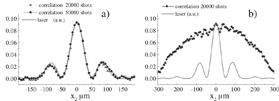

In a second set of measurements the source size is reduced to , by inserting a small pinhole after the ground glass. As a result, the spatial coherence of the light illuminating the object is increased. As the speckle size at the diaphragm is now , on average the object is illuminated by a single speckle of size much larger than the slit separation. The results are reported in the second row of Fig.4. As expected mandel:1995 the interference fringes are now visible in the instantaneous intensity distribution of the object beam 1 [frame (d)], and become sharper after averaging over some hundreds of shots [frame (e)]. Notice that the shape of the interference pattern is now elongated in the vertical direction, because the light emerging from the small source is not collimated. Horizontal sections of , plotted in Fig.6b, show a very good agreement with the diffraction pattern from laser illumination. Instead, no interference fringes at all appear in the correlation function of the intensities in the two arms, when plotted as a function of [frame (f)]. Notice that in this set of measurements the turbid medium was removed in order to increase the power. This is feasible in this case, because the very small size of the source allows a large number of independent patterns to be generated in a single tour of the glass disk.
Figures 4,5,6 evidence a remarkable complementarity between the observation of interference fringes in the correlation function (ghost diffraction), and in the intensity distribution of the object beam (ordinary diffraction). It also shows the fundamental role played by the spatial incoherence of the source in producing a ghost diffraction pattern: the more incoherent is the source, the more the two beams are spatially correlated and the more information about the object is available in the ghost diffraction pattern. The more coherent is the source, the flatter is the spatial correlation function of the two beams and the less information about the object is contained in the ghost diffraction. This is completely analogous to the complementarity between the one-photon and two-photon interference in Young’s double slit experiments with photons from a PDC source abouraddy:2001c, which was explained as a complementarity between coherence and entanglement. In our case of thermal beams, the complementarity is rather between coherence and spatial correlation, showing that also in this respect the classical spatial correlation produced by splitting thermal light play the same role as entanglement of PDC photons.
These results can be easily understood by using the formalism developed in Sec.III, and in particular by inspection of Eq.(4)for the correlation function of the intensity fluctuations . In the limit of spatially coherent light the field correlation function becomes constant in space in the region of interest, and the two integrals in Eq.(4) factorize to the product of two ordinary imaging schemes, showing the diffraction pattern of the object only in the object arm 1. As a result, by plotting the correlation as a function of , no object diffraction pattern can be observed, that is, no ghost diffraction occurs. The same observation can be made with respect to , and , explaining thus the analogy between the role of light coherence in the PDC and in the thermal case.
In general, the result of a correlation measurement is obtained by inserting into Eq. (4) the propagators that describe the ghost diffraction setup: , with being the object transmission function, and . We get
| (11) |
where is the amplitude of the diffraction pattern from the object. The result of a correlation measurement is a convolution of the diffraction pattern amplitude with the second order correlation function in the far-field. Hence the far-field coherence length determines the spatial resolution in the ghost diffraction scheme: the smaller the far-field speckles, the better resolved is the pattern. In the limit of speckles much smaller than the scale of variation of the diffraction pattern
| (12) |
Since the amplitude of the object diffraction pattern is involved in Eq.(11), ghost diffraction of a pure phase object can be realized with spatially incoherent pseudo-thermal beams, a possibility which was questioned in a recent letter abouraddy:2004.
VI The ghost image: tradeoff between resolution and visibility
By simply inserting the lens in the reference arm (see Fig.1), without changing anything in the object arm, we now pass to the ghost image. As it was predicted in thermal-oe, and experimentally demonstrated in ferriexp-osa, the result of cross-correlating the intensities of the reference and object arm is now the image of the object, shown e.g. in Fig. 7a.
Two issues are important in any imaging scheme: the spatial resolution and the signal-to-noise ratio.
As pointed out in thermal-oe; ferriexp-osa, the resolution capabilities of the ghost image setup are determined by the near field coherence length (the size of the near-field speckles). This can be easily understood by inserting the propagator , into Eq. (4):
| (13) |
which shows that the result of a correlation measurement in this setup is a convolution of the object transmission function with the near-field correlation function . In the following we shall consider a bucket detection scheme, where the reference beam intensity is correlated to the total photon counts in the object arm, that is, in practice to the sum of photo counts over a proper set of pixels. This makes the imaging incoherent bache:2004a, because it amounts to measuring
| (14) |
If we take the limit of spatially coherent light, where can be considered as constant over the whole beam size, Both Eqs. (13),(14) show that no information about the object image can be obtained by scanning . Conversely in the limit of spatially incoherent light where the speckle size is much smaller than the scale of variation of the object, , and both Eqs. (13),(14) converge to .
Concerning the signal-to-noise ratio, the discussion in Sec. III pointed out that it is determined by the image visibility. We have studied the visibility of the ghost image of a double slit in a sequence of measurements where the vertical size of the apertures was progressively reduced, while leaving unchanged their horizontal size and separation. This is shown in Fig.7a, where all the frames display the correlation function measured in a bucket detection scheme as a function of the reference pixel position . Despite the fact that all the frames have been obtained with the same number of averages , the sequence display a remarkable enhancement of the visibility as the object area is reduced.

This enhancement is more clearly visible in the horizontal sections plotted in Fig. 7b, where in each point the correlation function has been normalized to , so that the numbers on the vertical axis give directly the visibility [see Eq. (7)]. We notice that the visibility increases as the object area decreases, and correspondingly the the signal-to-noise-ratio increases, as expected.
In order to understand the origin of the behaviour shown in Fig.7, we need first to consider Eq.(14), that gives the correlation function in the bucket detection scheme. Let us assume that the object simply transmits the light over a region of area and stops it elsewhere. By assuming that the coherence length is smaller than the object features, as it is necessary for the object to be resolved, the integrand at r.h.s of (14) can be non-zero for in a region located around , of area , where is the coherence area . Thus the correlation scales as the coherence area.
| (15) |
Conversely, it is not difficult to see that in the bucket detection scheme
| (16) |
where is the average intensity distribution of the light illuminating the object, that can be taken as roughly uniform on the object area (the speckles average to a broad uniform light spot, as shown in Fig. 4b). Hence the ratio of the correlation to the background scales as:
| (17) |
This formula is reminiscent of role of the mode degeneracy in Eq.(8), and indeed it reflects the fact that in a bucket detection scheme the number of spatial modes detected is proportional to , which represents a degeneracy factor that reduces the visibility of the correlation with respect to the background. The ratio in Eq. (17) is usually small, so that the visibility of the ghost image roughly coincides with it. Thus the visibility roughly scales as the ratio of the coherence area to the object transmissive area: the larger are the object dimensions with respect to the speckles, that is, the more incoherent is the light illuminating the object, the worse is the visibility of the ghost image. This is confirmed by the plot in Fig. 8, showing how the visibility increases with the inverse of the object area.

This rather counter-intuitive result also implies that a better resolution can be achieved only at the expenses of the visibility, since the resolution is determined by the speckle size. Hence, complex images that need small speckles to be resolved in their details have a lower signal-to-noise ratio than simple images which can be resolved with relatively large speckles (see also valencia:2004 for a similar conclusion). This, however, does not prevent from retrieving more complex images (see e.g. Fig. 9), provided that a larger number of data acquisitions are performed.

VII Numerical results
In this section we use a numerical model for simulating the speckle pattern created by the ground glass and the turbid medium, as to support the results of the previous section. The thermal field is created by generating a noisy field with huge phase fluctuations. We then multiply the noisy field with a Gaussian profile and a subsequent Fourier transformation gives what corresponds to the near field; the width of the Gaussian then controls the near-field speckle size. The far-field speckle size is controlled independently as in the experiment: after generating the near field, a diaphragm of diameter is introduced, beyond which only vacuum fluctuations appear; then controls the far-field speckle size. The speckle field transmitted by the diaphragm is then impinged on a 50/50 BS, with vacuum fluctuations entering the unused port, giving the two desired correlated beams. We neglect the temporal statistics, since we assume that the short measurement time of the experiment provides a speckle pattern frozen in time. We should finally mention that a Wigner formalism is used to describe the quantized fields, as described in detail in brambilla:2004.

Initially, let us briefly show that the numerical simulations are able to describe very precisely the experiment. In Fig. 10 is shown the results of two-dimensional (2D) simulations with all parameters kept as close as possible to the experiment. This includes near-field and far-field speckle sizes, object and aperture sizes, as well as number of realizations. Both the ghost diffraction pattern [Fig. 10(a)] and the ghost image [Fig. 10(b)] show very good agreement with the experimental recorded data (using the small-speckle setup of Secs. IV- VI). We stress that this comparison is not in arbitrary units.

In Sec. V we showed experimentally the behaviour of the system when using either coherent or incoherent beams to investigate the diffraction properties of an object. In order to investigate better the actual transition from coherent to incoherent illumination of the object, we have carried out numerical simulations that are presented in Fig. 11. We have there kept mm and then for each simulation changed . The simulation only includes one spatial direction (1D), and therefore the coherence properties of the beam is governed by the ratio , where is the 1D equivalent of . Thus, the smaller the more incoherent is the beam impinging on the object. For small speckles () the beams are spatially incoherent, implying a strong spatial correlations between the beams: the ghost diffraction is observed in the correlation [Fig. 11(a)]. In contrast, no diffraction pattern can be observed directly in the object beam [Fig. 11(b)]. As is increased by generating bigger speckles the beams become more and more spatially coherent (): the ghost diffraction disappears gradually [Fig. 11(a)], while the diffraction pattern starts to appear from the direct observation of the object beam [Fig. 11(b)]. Figure 11(c) shows what happens for the ghost image during this transition: the incoherence for small implies that a ghost image of the object can be observed, and it disappears gradually while increasing the coherence.
We saw in Sec. VI that the visibility of the ghost image became better as the object area was reduced, cf. Fig. 8. To investigate this phenomenon in general we show in Fig. 12 how the object size22 2 Note that we here keep the length perpendicular to the slits constant but vary the width of the slits. Experimentally, this would correspond to maintaining the needle but changing the width of the surrounding aperture. effects the visibility of the information. The trend we saw in the experiment is repeated in the numerics: in Fig. 12(a) the ghost image visibility increases as the object size decreases because fewer modes are transmitted. In Fig. 12(b) the simulation is repeated for the 1D case with a similar result. However, since in the 1D case much fewer modes are transmitted by the object the visibility is much higher. We have also in Fig. 12 plotted the visibility of the ghost diffraction fringes, and we observe that – in contrast to the ghost image case – the visibility decreases as the object size is decreased. This is is to be expected because for the diffraction pattern the modes transmitted by the object interfere coherently so (for the 2D case). In contrast, for the mean intensity the modes interfere incoherently so . Thus : the bigger the object the better the visibility of the information. We also note that there is basically no difference between the 1D and 2D results for the ghost diffraction visibility. This is because a similar argument can be done for the 1D case showing . Finally, we have checked that if the far-field speckle size is varied and all other parameters are kept fixed, then the visibility of the diffraction fringes increases as is increased: again a tradeoff between resolution and visibility is found.

VIII Conclusions
The experimental results reported in this paper confirms that correlated imaging can be performed with a classical thermal source. A remarkable complementarity between spatial coherence and correlation is predicted and confirmed by experiments and numerical simulations. By changing the coherence of the speckle field at the object plane from incoherent to coherent (measured relative to the object dimensions), the object diffraction pattern reconstructed from correlations disappears while it appears in the far field intensity distribution measured in the object arm. We also discussed from a quantitative point of view the issue of the visibility of the correlated imaging scheme. We showed that the visibility of the object image is proportional to the ratio between the object area and the field coherence area at the object plane. This means that a tradeoff between resolution and visibility exists: a better visibility can be obtained only at the expense of a lower resolution and vice versa. However, the experiment clearly shows that a fairly good resolution can be achieved since the problem of low visibility can be overcome by performing a sufficiently large number of averages.
Acknowledgments
This work was carried out in the framework of the FET project QUANTIM of the EU, of the PRIN project of MIUR ”Theoretical study of novel devices based on quantum entanglement”, and of the INTAS project ”Non-classical light in quantum imaging and continuous variable quantum channels”. M.B. acknowledges financial support from the Carlsberg Foundation.
References
- (1) D. V. Strekalov, A. V. Sergienko, D. N. Klyshko, and Y. H. Shih, “Observation of Two-Photon ”Ghost” Interference and Diffraction,” Phys. Rev. Lett. 74, 3600–3603 (1995).
- (2) P. H. Souto Ribeiro, S. Padua, J. C. Machado da Silva, and G. A. Barbosa, “Controlling the degree of visibility of Young’s fringes with photon coincidence measurements,” Phys. Rev. A 49, 4176–4179 (1994).
- (3) T. B. Pittman, Y. H. Shih, D. V. Strekalov, and A. V. Sergienko, “Optical imaging by means of two-photon quantum entanglement,” Phys. Rev. A 52, R3429–R3432 (1995).
- (4) A. F. Abouraddy, B. E. A. Saleh, A. V. Sergienko, and M. C. Teich, ”Role of Entanglement in two photon imaging,” Phys. Rev. Lett. 87, 123602 (2001); ”Entangled-photon Fourier optics,” J. Opt. Soc. Am. B 19, 1174 (2002).
- (5) R. S. Bennink, S. J. Bentley, and R. W. Boyd, “”Two-Photon” Coincidence Imaging with a Classical Source,” Phys. Rev. Lett. 89, 113601 (2002).
- (6) A. Gatti, E. Brambilla, and L. A. Lugiato, “Entangled Imaging and Wave-Particle Duality: From the Microscopic to the Macroscopic Realm,” Phys. Rev. Lett. 90, 133603 (2003).
- (7) R. S. Bennink, S. J. Bentley, R. W. Boyd, and J. C. Howell, “Quantum and Classical Coincidence Imaging,” Phys. Rev. Lett. 92, 033601 (2004).
- (8) E. Brambilla, A. Gatti, M. Bache, and L. A. Lugiato, “Simultaneous near-field and far field spatial quantum correlations in the high gain regime of parametric down-conversion,” Phys. Rev. A 69, 023802 (2004).
- (9) J. C. Howell, R. S. Bennink, S. J. Bentley, and R. W. Boyd, “Realization of the Einstein-Podolsky-Rosen Paradox Using Momentum- and Position-Entangled Photons from Spontaneous Parametric Down Conversion,” Phys. Rev. Lett. 92, 210403 (2004).
- (10) M. D’Angelo, Y.-H. Kim, S. P. Kulik, and Y. Shih, “Identifying Entanglement Using Quantum Ghost Interference and Imaging,” Phys. Rev. Lett. 92, 233601 (2004), quant-ph/0401007.
- (11) A. Gatti, E. Brambilla, M. Bache, and L. A. Lugiato, ”Ghost imaging with thermal light: comparing entanglement and classical correlation,” Phys. Rev. Lett. 93, 093602 (2004), quant-ph/0307187; ”Correlated imaging, quantum and classical,” Phys. Rev. A 70, 013802 (2004), quant-ph/0405056.
- (12) D. Magatti, F. Ferri, A. Gatti, E. Brambilla, M. Bache, and L. A. Lugiato, ”Experimental evidence of high-resolution ghost imaging and ghost diffraction with classical thermal light,” quant-ph/0408021; F. Ferri, D. Magatti, A. Gatti, E. Brambilla, M. Bache, and L. A. Lugiato, ”High-resolution ghost image and ghost diffraction experiments with thermal light,” to appear in Phys. Rev. Lett. (2004).
- (13) Y. Cai and S.-Y. Zhu, “Ghost interference with partially coherent radiation,” Optics Letters 29, 2716 (2004).
- (14) D.-Z. Cao, Z. Li, Y.-H. Zhai, and K. Wang, “One-Photon and Two-Photon Double-Slit Interferences in Spontaneous and Stimulated Parametric Down-Conversions,” (2004), quant-ph/0401109.
- (15) J. Cheng and S. Han, “Incoherent Coincidence Imaging and Its Applicability in X-ray Diffraction,” Phys. Rev. Lett. 92, 093903 (2004).
- (16) G. Scarcelli, A. Valencia, and Y. Shih, “Experimental study of the momentum correlation of a pseudothermal field in the photon-counting regime,” Phys. Rev. A 70, 051802(R) (2004), quant-ph/0409210.
- (17) A. Valencia, G. Scarcelli, M. D’Angelo, and Y. Shih, “Two-photon imaging with thermal light,” Phys. Rev. Lett. 94, 063601 (2005), quant-ph/0408001.
- (18) A. F. Abouraddy, P. R. Stone, A. V. Sergienko, B. E. A. Saleh, and M. C. Teich, “Entangled-Photon Imaging of a Pure Phase Object,” Phys. Rev. Lett. 93, 213903 (2004).
- (19) A. N. Boto, P. Kok, D. S. Abrams, S. L. Braunstein, C. P. Williams, and J. P. Dowling, “Quantum Interferometric Optical Lithography: Exploiting Entanglement to Beat the Diffraction Limit,” Phys. Rev. Lett. 85, 2733 (2000).
- (20) M. D’Angelo, M. V. Chekhova, and Y. Shih, “Two-Photon Diffraction and Quantum Lithography,” Phys. Rev. Lett. 87, 013602 (2001).
- (21) K. Wang and D.-Z. Cao, “Subwavelength coincidence interference with classical thermal light,” Phys. Rev. A 70, 041801R (2004), quant-ph/0404078.
- (22) G. Scarcelli, A. Valencia, and Y. Shih, “Two-photon interference with thermal light,” Europhys. Lett. 68, 618–624 (2004), quant-ph/0410217.
- (23) R. Hanbury-Brown and R. Q. Twiss, “Correlations between photons in 2 coherent beams of light,” Nature (London) 177, 27 (1956).
- (24) J. W. Goodman, “Statistical properties of laser speckle patterns,” in Laser speckle and related phenomena, Vol. 9 of Topics in Applied Physics, D. Dainty, ed., (Springer, Berlin, 1975), p. 9.
- (25) W. Martienssen and E. Spiller, “Coherence and Fluctuations in Light Beams,” Am. J. Phys. 32, 919 (1964).
- (26) F. T. Arecchi, “Measurement of the Statistical Distribution of Gaussian and Laser Sources,” Phys. Rev. Lett. 15, 912 (1965).
- (27) J. Cheng and S. Han, “Theoretical investigation of the quantum noise in ghost imaging,” (2004), quant-ph/0408123.
- (28) L. Mandel and E. Wolf, Optical coherence and quantum optics (Cambridge, New York, 1995).
- (29) J. W. Goodman, Statistical optics (Wiley Classic Library, New York, 2000).
- (30) M. Bache, E. Brambilla, A. Gatti, and L. A. Lugiato, “Ghost imaging schemes: fast and broadband,” Opt. Express 12, 6067 (2004), quant-ph/0409215.
- (31) A. F. Abouraddy, M. B. Nasr, B. A. Saleh, A. V. Sergienko, and M. C. Teich, “Demonstration of the complimentarity of one- and two-photon interference,” Phys. Rev. A 63, 063803 (2001).