Quantum and Fisher Information from the Husimi and Related Distributions
Abstract
The two principal/immediate influences — which we seek to interrelate here — upon the undertaking of this study are papers of Życzkowski and Słomczyński (J. Phys. A 34, 6689 [2001]) and of Petz and Sudár (J. Math. Phys. 37, 2262 [1996]). In the former work, a metric (the Monge one, specifically) over generalized Husimi distributions was employed to define a distance between two arbitrary density matrices. In the Petz-Sudár work (completing a program of Chentsov), the quantum analogue of the (classically unique) Fisher information (montone) metric of a probability simplex was extended to define an uncountable infinitude of Riemannian (also monotone) metrics on the set of positive definite density matrices. We pose here the questions of what is the specific/unique Fisher information metric for the (classically-defined) Husimi distributions and how does it relate to the infinitude of (quantum) metrics over the density matrices of Petz and Sudár? We find a highly proximate (small relative entropy) relationship between the probability distribution (the quantum Jeffreys’ prior) that yields quantum universal data compression, and that which (following Clarke and Barron) gives its classical counterpart. We also investigate the Fisher information metrics corresponding to the escort Husimi, positive-P and certain Gaussian probability distributions, as well as, in some sense, the discrete Wigner pseudoprobability. The comparative noninformativity of prior probability distributions — recently studied by Srednicki (Phys. Rev. A 71, 052107 [2005]) — formed by normalizing the volume elements of the various information metrics, is also discussed in our context.
pacs
Valid PACS 03.67.-a, 02.50.Tt, 02.50.Sk, 02.40.KyI Introduction
The two-level quantum systems (TLQS) are describable (nonclassically) in terms of density matrices () — Hermitian nonnegative definite matrices of trace unity. These matrices can be parametrized by points in the unit ball (Bloch ball/sphere (Mosseri and Dandoloff 2001, p. 10244)) in Euclidean 3-space. On the other hand, the TLQS can be described in a classical manner using a generalization of the Husimi distribution Husimi 1940 (Życzkowski and Słomczyński 2001, sec. 4.1) (cf. Guiasu 1987; Levine 1988; Bach 1979; Bach 1980; Bach 1981; Gibbons 1992). “The Husimi function is a function on phase space, and takes only non-negative values while the Wigner function can be negative and is usually violently oscillating. Hence the Husimi function can be regarded as a probability distribution in phase space, and its order of delocalization can be a measure of chaoticity of quantum states” Sugita and Aiba 2002. (Note that the original Husimi distribution was defined only for density operators in separable Hilbert space — one which admits a countable orthonormal basis — while the distribution to be studied here is defined over a finite-dimensional Hilbert space.)
There is an (uncountable) infinitude (Penrose 2005, sec. 16.7) of (quantum monotone) Riemannian metrics that can be attached to the Bloch ball of TLQS. Contrastingly, in the classical context of the Husimi distribution, there is not an infinitude, but rather a single distinguished (up to a constant multiple) monotone Riemannian metric — the Fisher information metric Chentsov 1982; Campbell 1986; Frieden 2004. (“In the classical case, decision theory provides a unique montone metric, namely, the Fisher information. In the quantum case, there are infinitely many monotone metrics on the state space” (Petz and Sudár 1996, p. 2672).) So, it appears to be an question of obvious interest — which we seek to address here — of how one reconciles/deals with this phenomenon of classical uniqueness and quantum non-uniqueness, as applied to essentially the same objects (that is, the TLQS).
II Monotone metrics
The monotone metrics are all stochastically monotone Petz and Sudár 1996. That is, geodesic distances (as well as relative entropies) between density matrices decrease under coarse-grainings (completely positive trace-preserving maps, satisfying the Schwarz inequality: ). These metrics can be used for purposes of statistical distinguishability Petz and Sudár 1996. The monotone metrics for the TLQS have been found to be rotationally invariant over the Bloch ball, depending only on the radial coordinate , that is the distance of the state in question from the origin — corresponding to the fully mixed state. They are splittable into radial and tangential components of the form (Petz and Sudár 1996, eq. (3.17)),
| (1) |
Here, using spherical coordinates (), one has . Further, is an operator monotone function such that for every . (A function is operator monotone if the relation , meaning that is nonnegative definite, implies for any such matrices and of any order.) The radial component is independent of the function , and in the case of the Bures (minimal monotone) metric (corresponding to the particular choice ), the tangential component is independent of Hall 1998.
In the classical context of the Husimi distribution, there is not an infinitude, but rather a single distinguished (up to a constant multiple) monotone metric — the Fisher information metric Chentsov 1982; Campbell 1986; Frieden 2004. (The counterpart here to stochastic mappings — which are the appropriate morphisms in the category of quantum state spaces — are stochastic matrices Petz and Sudár 1996.) The -entry of the Fisher information matrix (tensor) is the expected value with respect to the probability distribution in question of the product of the first derivative of the logarithm of the probability with respect to its -th parameter times the analogous first derivative with respect to its -th parameter. (Under certain regularity conditions, the Fisher information matrix is equal to the “second derivative matrix for the informational divergence (relative entropy)” (Clarke and Barron 1990, pp. 455-456), (Clarke and Barron 1994, p. 43).) The volume element of the Fisher information metric can be considered — in the framework of Bayesian theory — as a prior distribution (Jeffreys’ prior Clarke and Barron 1990; Slater 1996a; Kwek et al. 1999) over, for our purposes here, the Bloch ball of TLQS.
II.1 Fisher information metric for the Husimi distribution
We have found (having to make use of numerical, as well as symbolic MATHEMATICA procedures in our quest) that for the Husimi distribution over the TLQS, the Fisher information metric takes the specific form (cf. (2)),
| (2) |
Here,
| (3) |
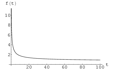
Now, a plot (Fig. 1) shows to be, in fact, a monotone function. ( is “almost” equal to .) It has a singularity at , corresponding to the fully mixed state (), where , though we have not attempted to confirm its operator monotonicity. Also, fulfills the self-adjointness condition of Petz and Sudár (Petz and Sudár 1996, p. 2667), at least at . For the pure states, that is , we have .

We further have the relation,
| (4) |
where is a specific “Morozova-Chentsov” function. There exist one-to-one correspondences between Morozova-Chentsov functions, monotone metrics and operator means (Petz 1996, Cor. 6). “Operator means are binary operations on positive operators which fulfill the main requirements of monotonicity and the transformer inequality” Petz 1996.
We can write (1) more explicitly as
| (5) |
Certainly, does not have — in terms of the radial component — the specific form (1) required of a monotone metric (cf. Slater 2000). In Fig. 2 we show both the radial components of (any) and of .

Petz (Petz 2002, p. 934) attributes the unvarying nature () of the radial component of the (quantum) monotone metrics to the (classical) Chentsov uniqueness (of Fisher information) theorem Chentsov 1982; Campbell 1986. “Loosely speaking, the unicity [sic] result in the [probability] simplex case survives along the diagonal and the off-diagonal provides new possibilities for the definition of a stochastically invariant metric” (Petz and Sudár 1996, p. 2664).
If we (counterfactually) equate the volume element of to that of a generic monotone metric (1), and solve for , we obtain a monotonically-decreasing function (Fig. 3) (cf. Slater 2000),
| (6) |
Converting to cartesian coordinates , the trace of can be simply expressed as , where (cf. Luo 2001; Frieden 2004). Also, at the fully mixed state (), the metric is simply flat, that is
| (7) |
(The Riemann and Ricci tensors evaluated at the fully mixed state have no non-zero entries.)
Numerical evidence indicates that the Fisher information matrix for the Husimi distribution over the TLQS is bounded by the corresponding information matrices for the (quantum) monotone metrics, in the sense that the monotone metric tensors minus the Fisher-Husimi information tensor are positive definite.
We can normalize the volume element of to a probability distribution by dividing by the Fisher information metric volume . If we generate a “hybridized-Husimi” (quantum Petz and Sudár 1996) monotone metric, , via the formula (1), using , then the volume of the Bloch ball of TLQS in terms of this newly-generated monotone metric is . Using this as a normalization factor, we obtain a probability distribution () of interest over the TLQS.
III Comparative Noninformativities
Let us compare — in the manner employed in Slater 1998; Clarke 1996 (cf. (Srednicki 2005; Slater, sec. VI)) — with the prior probability distribution (). The latter is gotten by normalizing the volume element of the well-studied minimal monotone (Bures) metric ((Slater 1996b, eq. (7)) (Slater 1996c, eq. (16))), that is,
| (8) |
generated from (1) using the operator monotone function . (We avoid the specific designations and because these are usually, confusingly, considered to generate the maximal and minimal monotone metrics, respectively (Petz and Sudár 1996, eq. (3.21)). Our integrations of probability distributions are conducted over and .)
The relative entropy (Kullback-Leibler distance) of with respect to [which we denote ] — that is, the expected value with respect to of — is 0.130845 “nats” of information. (We use the natural logarithm, and not 2 as a base, with one nat equalling 0.531 bits.) Let us note that the Shannon entropy () of the Husimi distribution is the Wehrl entropy () of the corresponding quantum state. Explicitly implementing (Mintert and Życzkowski 2004, eq. (6)), we have for the TLQS,
| (9) |
is always greater than the von Neumann entropy, , which for the TLQS is expressible as
| (10) |
(We, of course, notice the omnipresence in these last two formulas, as well as in (5) and further formulas below of the term . The two eigenvalues [] of are , so is expressible as .) Each monotone metric can be obtained in the form of a “contrast functional” for a certain convex subset of relative entropies Lesniewski and Ruskai 1999; Jenc̆ová 2004.
III.1 Bures prior
Now, let us convert to a posterior probability distribution () by assuming the performance of six measurements, two (with one outcome “up” and the other “down”) in each of the - and -directions. Normalizing the product of the prior and the likelihood function corresponding to the six measurement outcomes (Slater 1998, p. 3),
| (11) |
we find . (The cartesian coordinates in (11) are transformed to the spherical ones employed in our analysis.) So, in this sense is more noninformative than , the relative entropy being reduced by adding information to . On the other hand, — corresponding to the minimal monotone metric — is itself the least noninformative of the monotone-metric priors () Slater 1998. (Luo has established an inequality between the [monotone metric] Wigner-Yanase skew information and its minimal monotone counterpart Luo 2003.)
Reversing the arguments of the relative entropy functional, we obtain . But now, following the same form of posterior construction, we find , further supportive of the conclusion that is more noninformative than . In some sense, then, assumes less about the data than . But this diminishability of the relative entropy is limited. If we convert to a new posterior using the square of the likelihood function above — that is, assuming twelve measurements, four (with two outcomes “up” and the other two “down”) in each of the - and -directions, giving
| (12) |
then . To much the same effect, if we use a likelihood based on the optimal/nonseparable set of measurements for two qubits, consisting of five possible measurement outcomes, given in (Slater 2001, eq. (8)), to convert to a new posterior, then the relative entropy reaches higher still, that is from 0.130845 to 0.623855. (Employing a likelihood based on the optimal/nonseparable set of measurements for three qubits, consisting of eight possible measurement outcomes (Slater 2001, eq. (9)), the relative entropy with respect to increases further to 1.51365.) Actually, if we formally take in eq. (12), and renormalize to a new posterior, we obtain a superior reduction, that is, to . (Further, with , we get 0.0702389 and 0.0732039, with .)
III.2 Morozova-Chentsov prior
In Slater 1998, it was found that the (“Morozova-Chentsov”) prior distribution,
| (13) |
that is, the normalized volume element of the monotone metric (1) based on the operator monotone function,
| (14) |
was apparently the most noninformative of those (normalizable) priors based on the operator monotone functions that had been explicitly discussed in the literature. Now, , that is, quite large. This can be reduced to 0.893996 if, into , one incorporates measurements of the type described above; diminished further to 0.561901 with ; and further still to 0.471852 — the greatest reduction of this type — with . (For , it starts to rise to 0.652441.)
But, if we again use the likelihood based on the optimal nonseparable measurement of two qubits (Slater 1998, eq. (8)), with just five measurements, the relative entropy of the corresponding posterior form of with respect to is reduced to 0.342124, which is the smallest we have achieved so far along these lines. (For the mentioned optimal nonseparable measurement scheme for three qubits, the reduction is quite minor, only to 1.33492 nats.) We obtained intermediate-sized reductions to 0.45524 and 0.492979, respectively, by using for our measurements, twenty projectors oriented to the vertices (Decker et al. 2004, secs. 9, 10) of a dodecahedron and of an icosahedron. (The primary measurement scheme used above, and in Slater 1998, with six measurements oriented along three orthogonal directions, is tantamount to the use of an octahedron.)
III.3 Hilbert-Schmidt prior
The prior distribution generated by normalizing the volume element of the Hilbert-Schmidt metric over the Bloch sphere is (Slater 1998, eq. (10)) (Hall 1998, eq. (31))
| (15) |
which is simply the uniform distribution over the unit ball. The Hilbert-Schmidt volume element can be reproduced using the formula (1) for a quantum monotone metric, making use of , but this function is neither monotone-increasing nor decreasing over (cf. Ozawa 2001).
We have that and . Now, in terms of our usual posterior distributions based on six measurements, and , so we can conclude that the Husimi prior is more noninformative than the Hilbert-Schmidt prior .
IV Universal Data Compression
Employing as a prior distribution (Jeffreys’ prior) over the family (Riemannian manifold) of Husimi qubit probability distributions, the (classical) asymptotic minimax/maximin redundancy of universal data compression is equal to (Clarke and Barron 1994, eq. (2.4)) Clarke and Barron 1990,
| (16) |
where is the sample size (the number of qubits [TLQS]) and we used the before-mentioned volume of . (“Suppose that is a discrete random variable whose distribution is in the parametric family and we want to encode a block of data for transmission. It is known that a lower bound on the expected codeword length is the entropy of the distribution. Moreover, this entropy bound can be achieved, within one bit, when the distribution is known. Universal codes have expected length near the entropy no matter which member of the parametric family is true. The redundancy of a code is defined to be the difference between its expected length and its entropy” (Clarke and Barron 1990, p. 459).)
For the quantum/nonclassical counterpart Krattenthaler and Slater 2000 (cf. Hayashi and Matsumoto 2002; Jozsa and Presnell 2003; Jozsa et al. 1998), let us consider the use of the “Grosse-Krattenthaler-Slater” (“quasi-Bures”) probability distribution (Slater 2001, eq. (33)),
| (17) |
This is the normalized form of the monotone metric (1) associated with the (presumably operator) monotone function,
| (18) |
(Taking limits, we have for the fully mixed state, and for the pure states, .) It appears Grosse et al. (though not yet fully rigorously established) that the (quantum) asymptotic minimax/maximin redundancy, employing as a prior probability distribution over the density matrices (and their -fold tensor products (cf. Caves et al. 2002)), is . This is greater than the classical (Husimi-Fisher-information-based) analog (16) by 2.20095 nats of information. It would seem that this difference is attributable to the greater dimensionality () of an -qubit Hilbert space, as opposed to a dimensionality of for trivariate Husimi probability distributions over the TLQS.
We further note that and , both being very small. Smaller still, and — whence the designation . But then, even more strikingly, we computed that and . In Fig. 4 we show the one-dimensional marginal probability distributions over the radial coordinate of the five distributions , , , and , with those for and being — as indicated — particularly proximate.

Substitution of for into the quantum asymptotic (maximin) redundancy formula that has to be maximized over all possible prior probability distributions (Grosse et al., eq. (4.3)),
| (19) |
leads to a very slightly decreased (and hence suboptimal) redundancy, vs. . (Use of as a quantum prior over the density matrices gives us a constant term of , use of , and use of , .) To obtain the appropriate form of to use in (19), we take our probability distributions (such as (8) and (13)), divide them by and integrate the results over and . (Thus, we must have .) The minimax objective function is
| (20) |
The minimax is also achieved using the formed from .
We can, additionally, achieve an extremely good fit to by proceeding in somewhat an opposite fashion to that above — reversing our hybridization procedure. Employing , rather than in the expression (2) for and obtaining the corresponding normalized (dividing by 4.00277) volume element (), we find . (Interchanging the arguments of the relative entropy functional, we get 0.000317754.) It is quite surprising, then, that a joint plot of and readily shows them to be substantially different in character (for example, and ), since they have been shown here to generate two pairs of such highly similar probability distributions, one pair composed of (quantum) monotone ( and ), and the other pair of (quantum) non-monotone metrics ( and ).
V Escort-Husimi Distributions
For the escort-Husimi distributions Pennini and Plastino 2004, we raise the probability element of the Husimi distribution to the -th power, and renormalize to a new probability distribution. (Of course, the Husimi distribution itself corresponds to . If we set , we recover the -family of Amari Amari 1982; Naudts 2004; Jenc̆ová 2004.) To normalize the -th power of the Husimi distribution, one must divide by
| (21) |
V.1 The case
For (entropic index) , the Fisher information metric takes the form
| (22) |
where
| (23) |
We have and .
V.1.1 Relative entropies
Further, the relative entropies and , So, it appears that is even less noninformative than (recalling that ), which in turn we found above was less noninformative than the prior probabilities formed from any of the (quantum) monotone metrics. We also note that . If we “hybridize” by modifying its radial component into that required of a (quantum) monotone metric, then we find that is quite small.
V.2 The cases
For the escort-Husimi probability distribution with , the Fisher information metric takes the form
| (24) |
where
| (25) |
Now, and a plot of clearly manifests monotonic behavior also. (The monotonically-decreasing scalar curvature of equals at .) We have that , so the informativity (noninformativity) of the escort-Husimi prior probabilities appears to increase (decrease) with .
For ,
| (26) |
where
| (27) |
For ,
| (28) |
where
| (29) |
We have (as found by C. Krattenthaler, making use of explicit MATHEMATICA computations of ours for ) (cf. (Gnutzmann and Życzkowski 2001, sec. 3.2) Sugita 2003),
| (30) |
(For odd some simplification in the resulting expression occurs due to cancellation by a factor of .)
In Fig. 5 we plot , revealing their common monotonically-increasing behavior. (Of course, we have , shown already in Fig. 1. The steepness of the curves decreases with increasing .)

Let us further note that in addition to and , we have and . (We have also been able to compute that and .) So, the best of these fits of to the prior probabilities for the hybridized-escort-Husimi probability distributions is for .
V.3 Tangential components
Now, we can reexpress the formula (30) without summations, making use of the binomial theorem, as
| (31) |
So, we could study hybridized escort-Husimi metrics based on non-integral using this formula. (We note that (31), in fact, yields .) For example,
| (32) |
Thus, (31) gives us (following the formulation (1)) the tangential components of the escort-Husimi Fisher information metrics for arbitrary . (Pennini and Plastino Pennini and Plastino 2004 have argued, though, that in a quantal regime, can be no less than 1. Tsallis statistics with an entropic index of , Beck has contended, correctly describes the small-scale statistics of Lagrangian turbulence Beck 2001.)
V.4 Radial components
We do not have, at this point, a comparable complete formula for the radial components. However, C. Krattenthaler has shown — making use of explicit computations of ours for the cases — that the denominators of the functions giving the radial components are simply proportional to
| (33) |
(The Pochhammer symbol is synonymous with the rising or ascending factorial. The obtaining of comparable formulas for the numerators of the radial components might be possible using the “Rate.m” program available from the website of Krattenthaler [http://www.mat.univie.ac.at/ kratt/], if we had available additional explicit computations beyond the .) As way of illustration, the radial component of is expressible as
| (34) |
VI Positive P-Representation for TLQS
Braunstein, Caves and Milburn focused on a specific choice of positive P-representation which they called the canonical form and which is always well defined (Braunstein et al. 1991, eq. (3.3)) (cf. (Gardiner and Zoller 2004, sec. 6.4)):
| (35) |
“The canonical form is clearly positive, and…it is essentially the Q-function [Husimi distribution]” Braunstein et al. 1991.
We sought to implement this model, choosing for and independent 2-dimensional representations of the spin- coherent states (while for the Husimi distribution or Q-function, only, say , need be employed). (The “positive P representation achieves [its] considerable success by doubling the number of degrees of freedom of the system, i. e., doubling the number of dimensions of the phase space” (Braunstein et al. 1991, p. 1153). More typically, in the positive P-representation, and are allowed to vary independently over the entire complex plane.) However, then our result — using this choice of and — was not normalized to a probability distribution in the manner indicated in (35).
We noted that Braunstein, Caves and Milburn had commented that a “positive P representation can be defined for a large class of operators. We restrict ourselves here to those that are built up from the standard annihilation and creation operators of a harmonic oscillator. In particular, our work does not apply to generalizations of the positive P representation that include spin or pseudospin operators often used to describe a two-level atom” (Braunstein et al. 1991, p. 1155). (We are not aware, however, of any specific applications reported in the literature of the positive P-representation to -level [finite-dimensional] quantum systems.)
We did not perceive how to exactly (re)normalize the distribution (35) for our particular choices of and . So, we expanded just the exponential term of (35) into a power series in third order in the four phase variables and exactly normalized the product of this series with the remaining unmodified factor (the Q-function or Husimi distribution) to obtain a new (presumed) probability distribution. We then fit (numerically) the resultant tangential component of the associated Fisher information metric to the form (1) required of a monotone metric. In Fig. 6 we show what we (gratifyingly) obtained in this manner for .

In Fig. 7 we show an approximation to the radial component of , similarly obtained.

(The positive P-function “seems to possess some interesting properties and may deserve close inspection”(Lee 1995, p. 175).) It would be of interest to see how near the associated probability distributions ( and ) would be to the probability distributions (already discussed above) and . Most pressing, though, is the question of whether or not the concept of a positive P-representation does, in fact, have a meaningful and natural theoretical application to the -level quantum systems.
VII Gaussian Distribution
An approach quite distinct from that of the Husimi probability distributions, but still classical in nature, to modeling quantum systems has been presented in Guiasu 1987; Levine 1988; Bach 1979; Bach 1980; Bach 1981 (cf. Gibbons 1992). Here the family of probability distributions is taken as that of the Gaussian (complex multivariate normal distributions) having covariance matrix equal to the density matrix. For the TLQS, Slater (Slater 1995, eq. (13)) (Slater 1996d, eq. (16)) derived the corresponding Fisher information metric. This is representable as,
| (36) |
The tangential component can be reproduced, following the basic formula (1), by choosing . This is simply one-half of that — — associated with the maximal monotone (Yuen-Lax) metric Yuen and Lax 1973. Like that metric, the metric (36) yields a non-normalizable volume element (so one can not immediately apply — without some preliminary truncation — the comparative noninformativity/relative entropy test we have used above Slater 1998; Clarke 1996). Of course, the radial component of (36) is also not consistent with the requirement for a monotone metric. In fact, it rises much more steeply than , in opposite behavior to that for . In Fig. 8 we show this phenomenon.

VIII Discrete Wigner Function for a Qubit
The discrete Wigner function (pseudoprobability) , in the simplest case of a qubit, is defined on a array, with four components (Galvão 2005, eqs. (14)-(17)). The sum of in each “line” is the probability of projecting the state onto the basis vector , where indexes a set of three mutually unbiased bases (MUB) for a qubit and indexes the basis vector in each MUB. Choosing the MUB to be the eigenstates of the three Pauli operators, and using our cartesian coordinates, one can obtain three one-dimensional marginal (binomial) probability distributions over the and -axes, of the form (cf. Asplund and Björk 2001; Cunha et al. 2001). Now, the corresponding Jeffreys’ prior for the one-dimensional family of such binomial distribution is simply the beta distribution . (Let us note that the one-dimensional marginal distributions obtained for are of another form, that is, .)
Let us take the product of and , which naturally forms a (prior) probability distribution,
| (37) |
over the hypercube with vertices and renormalize/truncate it to a probability distribution over the Bloch sphere,
| (38) |
(Thus, the quantum-mechanically inaccessible region lying outside the Bloch ball, but within the hypercube is disregarded — assigned null measure — in the new normalization.)
Now, we found — strictly following the notation, formulas and line of argument above in sec. III — that and , so these two distributions are rather close in nature. Of course, is rotationally-symmetric over the Bloch sphere, while is not, so it seems to make little sense to try to compute some function to generate the tangential component. We found it problematical, using our usual (relative entropy) approach, to designate either or as more or less noninformative. (The “Husimi function is a kind of…coarse-grained Wigner function” (Sugita 2003, p. 3).)
IX Scalar curvature
In Fig. 9, we plot the scalar curvature of .

The formula for this scalar curvature is
| (39) |
where . Also, expanding about ,
| (40) |
The nonpositive monotonically-decreasing scalar curvature (Fig. 9) has its maximum at , corresponding to the fully mixed state, indicative of a flat metric there (cf. (7)) (and is at the pure states, ). For the minimal monotone (Bures) metric, the nonnegative scalar curvature is constant, that is , over the Bloch ball, and for the -dimensional convex set of density matrices, , achieves its minimum of at the fully mixed state () Dittmann 1999. (In Dittmann 1999, the metric used is one-quarter of that corresponding to (1), used here, so the results we compute here differ from those there by such a factor. For the maximal monotone metric, , which is monotonically-decreasing as increases, as is .)
For the two-level quantum sytems, Andai Andai 2003 has constructed a family of monotone metrics with non-monotone scalar curvature, and given a condition for a monotone metric to have a local minimum at the maximally mixed state.
IX.1 Metrics of constant scalar curvature
The metric has constant scalar curvature, , while, as previously noted, . Let us note that , which is also for . Here, WY denotes the Wigner-Yanase metric — the only pull-back metric among the quantum monotone metrics — and , which is the only self-dual operator monotone function Gibilisco and Isola 2003. “It is not known at the moment if there are other monotone metrics of constant sectional and scalar curvature” (Gibilisco and Isola 2003, p. 3760). It is a theorem that the “set of two-dimensional normalized density matrices equipped with the Bures metric is isometric to one closed-half of the three-sphere with radius ” Hübner 1992. The WY-metric “looks locally like a sphere of radius 2 of dimension ” (Gibilisco and Isola 2003, p. 3759). If we transform to spherical coordinates on the 3-sphere, then, the metric tensor for is diagonal in character, while the two other (constant scalar curvature) metrics are not (cf. Molnár and Timmermann 2003).
The three metrics and are Einstein. If we scale these metrics so that they are all of unit volume Gursky and LeBrun 1998, then and . The constant scalar curvatures of (unit-volume) Yamabe metrics are bounded above, and their least upper bound is a real number equal to , where is the volume of the standard metric on , and in our (Bloch sphere) case, , so the bound is Gursky and LeBrun 1998.
X Discussion
Luo Luo 2001 (cf. (Pennini and Plastino 2004, sec. 2.4) Twamley 1996; Slater 1996a; Kwek et al. 1999) has calculated the Fisher information matrix of the Husimi distribution in the Fock-Bargmann representation of the quantum harmonic oscillator with one degree of freedom. He found that the Fisher information of the position and that of the momentum move in opposite directions, and that a weighted trace of the Fisher information matrix is a constant independent of the wave function, and thus has an upper bound. (Luo did not consider the possibility of generating prior probability distributions by normalizing the volume element of the Fisher information metric.)
Gnutzmann and Życzkowski noted that one “is tempted to think of the Husimi function as a probability density on the phase space. However, the rules for calculating expectation values of some observable using the Husimi function are non-classical” (Gnutzmann and Życzkowski 2001, sec. 2.1) (cf. (Esposito et al. 2004, p. 548)). Gardiner and Zoller remarked that the “main problem of the Q-function is that not all positive normalizable Q-functions correspond to positive normalizable density operators” (Gardiner and Zoller 2004, p. 109).
Further, the comparison of distances between Husimi distributions for arbitrary quantum states based on the Fisher information metric with those employing the Monge distance Życzkowski and Słomczyński 2001, might be investigated. For the TLQS studied here, the Monge distance is, in fact, “consistent with the geometry of the Bloch ball induced by the Hilbert-Schmidt or the trace distance” (Życzkowski and Słomczyński 2001, p. 6716). (The trace distance is monotone, but not Riemannian, while the Hilbert-Schmidt distance, contrastingly, is Riemannian, but not monotone (Sommers and Życzkowski 2003, p. 10083) Ozawa 2001.) For -dimensional quantum systems (), unlike the trace, Hilbert-Schmidt or Bures distance, the Monge distance of to the fully mixed state — which provides information concerning the localization of in the classical phase space — is not the same for all pure states Życzkowski and Słomczyński 2001. The only monotone metrics for which explicit distance formulas are so-far available are the Bures (minimal monotone) and Wigner-Yanase ones Gibilisco and Isola 2003.
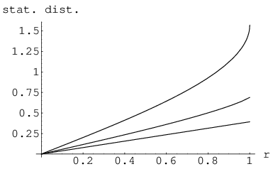
In Fig. 10 we show how the distance from the fully mixed state () increases as increases, for any monotone metric and for , and (linearly) for the Monge (or Hilbert-Schmidt) metric. The first-mentioned distance — taking the functional form (equalling for ) — dominates the second-mentioned distance (equalling for ), which in turns dominates the third (Życzkowski and Słomczyński 2001, eq. (4.10)), which takes the value for .
Let us bring to the attention of the reader, a recent preprint, which introduces a concept of escort density operators and a related one of generalized Fisher information Naudts 2005 (cf. Lutwak et al. 2005; Naudts 2004).
We have been consistently able above to find (apparently operator) monotone functions to generate the tangential components of (classical) Fisher information metrics for (rotationally-symmetric) probability distributions over the TLQS. We suspect the existence of some (yet not formally demonstrated) theorem to this effect. Also, it would be of interest to formally test the various monotone functions presented above for the property (requisite for a quantum monotone metric Petz and Sudár 1996; Petz 1996 of operator monotonicity.
We have “hybridized” above to a (quantum) monotone metric by replacing its radial component by that required (), while retaining its tangential component (formed from ). But it appears that we could also convert it by appropriately scaling (a conformal transformation) the entire metric (tangential and radial components) by some suitable function. If we do so, we find that — by explicit construction — the new metric () has the required radial component, while the tangential component is generated by a function
| (41) |
which also appears to be operator monotone. (We note that and .) But now, we have the large relative entropies and . At , is not flat, as is , but has a (limiting) scalar curvature of .
X.1 Further questions
Motivated by the analyses above, we would like to pose the question of whether there exists a family of trivariate probability distributions parametrized by the points of the Bloch ball, for which the associated (classically unique [up to a constant multiple]) Fisher information metric fully — both in terms of tangential and radial components – has the requisite form (1) for a monotone metric. Also, the volume elements (and hence associated prior probabilities) of the monotone metrics are expressible as the product of Haar measure and measures over the eigenvalues Hall 1998. To what extent, if any, does this hold true for prior probabilities not arising from monotone metrics? Are there any non-monotone metrics which give rise to prior probabilities more noninformative than (at the very least) the minimal monotone (Bures) one? What are suitable counterparts to formula (1) for -level quantum systems ()? Are there any monotone metrics which are flat at the fully mixed state, as is (7)?
XI Summary
In a classical context, for the family of Husimi probability distributions over the three-dimensional Bloch ball of two-level quantum systems (TLQS), we derived the (flat-at-the-fully-mixed-state) Fisher information metric (, given by (2)). Its tangential — but not its radial () — component conformed to that of one of the (uncountably) infinite class of (quantum) monotone metrics. The prior probability distribution () formed by normalizing the volume element of was found (sec. III.1) to be considerably less noninformative than the priors formed from any of the (quantum) monotone metrics, even that () based on the (relatively informative) minimal monotone (Bures) metric. However, if we replaced the radial component of by that required () of all (quantum) monotone metrics, the resultant “hybridized-Husimi” prior probability () became very close (in the sense of relative entropy “nats”) to , and thus comparably informative in nature, but even nearer () to another quantum-monotone-metric-based (“Grosse-Krattenthaler-Slater” or “quasi-Bures”) probability distribution () that has been conjectured to yield the asymptotic minimax/maximin redundancy for universal quantum coding. The analogous (Bayesian) role in universal (classical) coding — by a well-known result of Clarke and Barron Clarke and Barron 1990; Clarke and Barron 1994 — is played by Jeffreys’ prior (cf. Slater 1996a; Kwek et al. 1999). This takes the specific (original, non-hybridized) form for the family (manifold) of trivariate Husimi qubit probability distributions under study. We also studied the Fisher information metric for the escort-Husimi (sec. V), positive-P (sec. VI) and certain Gaussian probability distributions (sec VII), as well as, in some sense, the discrete Wigner pseudoprobability (sec. VIII). Additionally, we applied the Clarke comparative noninformativity test Slater 1998; Clarke 1996 to quantum priors (sec. III). Evidence that this test is consistent with the recently-stated criterion of “biasedness to pure states” of Srednicki Srednicki 2005 has been presented Slater.
References
- Mosseri and Dandoloff (2001) R. Mosseri and R. Dandoloff, J. Phys. A. 34, 10243 (2001).
- Husimi (1940) K. Husimi, Proc. Phys. Soc. Japan 22, 264 (1940).
- Życzkowski and Słomczyński (2001) K. Życzkowski and W. Słomczyński, J. Phys. A 34, 6689 (2001).
- Guiasu (1987) S. Guiasu, Phys. Rev. A 36, 1971 (1987).
- Levine (1988) R. D. Levine, J. Statist. Phys. 52, 1203 (1988).
- Bach (1979) A. Bach, Phys. Lett. A 73, 287 (1979).
- Bach (1980) A. Bach, J. Math. Phys. 21, 789 (1980).
- Bach (1981) A. Bach, J. Phys. A 14, 125 (1981).
- Gibbons (1992) G. W. Gibbons, J. Geom. Phys. 8, 147 (1992).
- Sugita and Aiba (2002) A. Sugita and H. Aiba, Phys. Rev. E 65, 036205 (2002).
- Penrose (2005) R. Penrose, The Road to Reality (A. A. Knopf, New York, 2005).
- Chentsov (1982) N. N. Chentsov, Statistical Decision Rules and Optimal Inference (Amer. Mat. Soc., Providence, 1982).
- Campbell (1986) L. L. Campbell, Proc. Amer. Math. Soc. 98, 135 (1986).
- Frieden (2004) B. R. Frieden, Science from Fisher Information: A Unification (Cambridge Univ, Cambridge, 2004).
- Petz and Sudár (1996) D. Petz and C. Sudár, J. Math. Phys. 37, 2662 (1996).
- Hall (1998) M. J. W. Hall, Phys.Lett.A 242, 123 (1998).
- Clarke and Barron (1990) B. S. Clarke and A. R. Barron, IEEE Trans. Info. Theory 36, 453 (1990).
- Clarke and Barron (1994) B. S. Clarke and A. R. Barron, J. Statist. Plann. Inference 41, 37 (1994).
- Slater (1996a) P. B. Slater, J. Phys. A 29, L601 (1996a).
- Kwek et al. (1999) L. C. Kwek, C. H. Oh, and X.-B. Wang, J. Phys. A 32, 6613 (1999).
- Petz (1996) D. Petz, Linear Alg. Applics. 244, 81 (1996).
- Slater (2000) P. B. Slater, Lett. Math. Phys. 52, 343 (2000).
- Petz (2002) D. Petz, J. Phys. A 35, 929 (2002).
- Luo (2001) S. Luo, J. Statist. Phys. 102, 1417 (2001).
- Slater (1998) P. B. Slater, Phys. Lett. A 247, 1 (1998).
- Clarke (1996) B. Clarke, J. Amer. Statist. Assoc. 91, 173 (1996).
- Srednicki (2005) M. Srednicki, Phys. Rev. A 71, 052107 (2005).
- (28) P. B. Slater, eprint quant-ph/0507203 (to appear in J. Phys. A).
- Slater (1996b) P. B. Slater, J. Phys. A 29, L271 (1996b).
- Slater (1996c) P. B. Slater, J.Math. Phys. 37, 2682 (1996c).
- Mintert and Życzkowski (2004) F. Mintert and K. Życzkowski, Phys. Rev. A 69, 022317 (2004).
- Lesniewski and Ruskai (1999) A. Lesniewski and M. B. Ruskai, J. Math. Phys. 40, 5702 (1999).
- Jenc̆ová (2004) A. Jenc̆ová, Intl. J. Theor. Phys. 43, 1635 (2004).
- Luo (2003) S. Luo, Proc. Amer. Math. Soc. 132, 885 (2003).
- Slater (2001) P. B. Slater, J. Phys. A 34, 7029 (2001).
- Decker et al. (2004) T. Decker, D. Janzing, and T. Beth, Intl. J. Quant. Inform. 2, 353 (2004).
- Ozawa (2001) M. Ozawa, Phys. Lett. A 268, 158 (2001).
- Krattenthaler and Slater (2000) C. Krattenthaler and P. B. Slater, IEEE Trans. Info. Theory 46, 801 (2000).
- Hayashi and Matsumoto (2002) M. Hayashi and K. Matsumoto, Phys. Rev. A 66, 022311 (2002).
- Jozsa and Presnell (2003) R. Jozsa and S. Presnell, Proc. Royal Soc. Lond. A 459, 3061 (2003).
- Jozsa et al. (1998) R. Jozsa, M. Horodecki, P. Horodecki, and R. Horodecki, Phys. Rev. Lett. 81, 1714 (1998).
- (42) H. Grosse, C. Krattenthaler, and P. B. Slater, Asymptotic redundancies for universal quantum coding. part 2 (in preparation).
- Caves et al. (2002) C. M. Caves, C. A. Fuchs, and R. Schack, J. Math. Phys. 43, 4537 (2002).
- Pennini and Plastino (2004) F. Pennini and A. Plastino, Phys. Lett. A 326, 20 (2004).
- Amari (1982) S. I. Amari, Ann. Statist. 10, 357 (1982).
- Naudts (2004) J. Naudts, J. Inequal. Pure Appl. Math. 5, 1 (2004).
- Gnutzmann and Życzkowski (2001) S. Gnutzmann and K. Życzkowski, J. Phys. A 34, 10123 (2001).
- Sugita (2003) A. Sugita, J. Phys. A 36, 9081 (2003).
- Beck (2001) C. Beck, Phys. Lett. A 287, 240 (2001).
- Braunstein et al. (1991) S. L. Braunstein, C. M. Caves, and G. J. Milburn, Phys. Rev. A 43, 1153 (1991).
- Gardiner and Zoller (2004) C. W. Gardiner and P. Zoller, Quantum Noise (Springer, Berlin, 2004).
- Lee (1995) H. W. Lee, Phys. Rep. 259, 147 (1995).
- Slater (1995) P. B. Slater, Phys. Lett. A 206, 66 (1995).
- Slater (1996d) P. B. Slater, Phys. A 223, 167 (1996d).
- Yuen and Lax (1973) H. P. Yuen and M. Lax, IEEE Trans. Info. Theory 19, 740 (1973).
- Galvão (2005) E. F. Galvão, Phys. Rev. A 71, 042302 (2005).
- Asplund and Björk (2001) R. Asplund and G. Björk, Phys. Rev. A 64, 012106 (2001).
- Cunha et al. (2001) M. O. T. Cunha, V. I. Man’ko, and M. O. Scully, Found. Phys. Lett. p. 103 (2001).
- Dittmann (1999) J. Dittmann, J. Geom. Phys. 31, 16 (1999).
- Andai (2003) A. Andai, J. Math. Phys. 44, 3675 (2003).
- Gibilisco and Isola (2003) P. Gibilisco and T. Isola, J. Math. Phys. 44, 3752 (2003).
- Hübner (1992) M. Hübner, Phys. Lett. A 163, 239 (1992).
- Molnár and Timmermann (2003) L. Molnár and W. Timmermann, J. Phys. A 36, 267 (2003).
- Gursky and LeBrun (1998) M. J. Gursky and C. LeBrun, GAFA Geom. Funct. Anal. 8, 965 (1998).
- Twamley (1996) J. Twamley, J. Phys. A 29, 3723 (1996).
- Esposito et al. (2004) G. Esposito, G. Marmo, and G. Sudarshan, From Classical to Quantum Mechanics (Cambridge Univ. Press, Cambridge, 2004).
- Sommers and Życzkowski (2003) H.-J. Sommers and K. Życzkowski, J. Phys. A 36, 10083 (2003).
- Naudts (2005) J. Naudts, Open Syst. Inform. Dyn. 12, 13 (2005).
- Lutwak et al. (2005) E. Lutwak, D. Yang, and G. Y. Zhang, IEEE Trans. Info. Theory 51, 473 (2005).