Adiabatic Approximation for weakly open systems

Patrik Thunström Email: patrik.thunstrom@kvac.uu.se Affiliation: Department of Quantum Chemistry, Uppsala University, Box 518, SE-751 20 Uppsala, Sweden Johan Åberg Email: johan.aaberg@kvac.uu.se Affiliation: Department of Quantum Chemistry, Uppsala University, Box 518, SE-751 20 Uppsala, Sweden Erik Sjöqvist Email: eriks@kvac.uu.se Affiliation: Department of Quantum Chemistry, Uppsala University, Box 518, SE-751 20 Uppsala, Sweden

August 11, 2026

Abstract

We generalize the adiabatic approximation to the case of open quantum systems, in the joint limit of slow change and weak open system disturbances. We show that the approximation is “physically reasonable” as under wide conditions it leads to a completely positive evolution, if the original master equation can be written on a time-dependent Lindblad form. We demonstrate the approximation for a non-Abelian holonomic implementation of the Hadamard gate, disturbed by a decoherence process. We compare the resulting approximate evolution with numerical simulations of the exact equation.

pacs

03.67.Lx, 03.65.Yz, 03.65.Vf

I Introduction

Recently, there has been a growing interest in the adiabatic theorem Messiah 1962 in the context of quantum information, in particular for fault tolerant holonomic quantum computation Zanardi and Rasetti 1999, and for the design of quantum adiabatic algorithms Farhi et al. 2000; Farhi et al. 2001. In this paper, we put forward a type of adiabatic approximation with focus on how an ideal (unitary) adiabatic evolution governed by a time-dependent Hamiltonian $H$ is perturbed by open-system effects. We consider the effects of a disturbance $D_{t/T}$ on a desired ideal evolution $\dot{\varrho}=-i[H(t/T),\varrho]$ , as a master equation $\dot{\varrho}=L_{t/T}\varrho=-i[H(t/T),\varrho]+\Gamma D_{t/T}(\varrho)$ , where $\Gamma$ gives the “strength” of the disturbance, and $T$ is the run-time. In the ideal case $\Gamma=0$ , the adiabatic approximation decouples the evolution of the instantaneous eigenspaces of $H$ . In the present approximation, the eigenspace structure of $H(t/T)$ still plays a role in that it determines what should decouple in the adiabatic limit. It turns out that this in general limits the applicability to systems that are weakly open, i.e., to small $\Gamma$ . The present study generalizes Refs. Romero et al. 2002; Pinto et al. 2002, as it allows degeneracy of the Hamiltonian, which is an essential feature to obtain non-Abelian holonomy effects in general Wilczek and Zee 1984 and holonomic quantum computation Zanardi and Rasetti 1999 in particular.

The concept of adiabaticity in open systems has been addressed recently by Sarandy and Lidar in Refs. Sarandy and Lidar 2005a; Sarandy and Lidar 2005 for master equations of the above type. In their approach, the adiabatic approximation is characterized by a decoupling in terms of instantaneous Jordan blocks of the superoperator $L_{t/T}$ . In other words, the decoupling is determined, in Ref. Sarandy and Lidar 2005a, by the total superoperator $L_{t/T}$ , while this is determined by $H(t/T)$ in the present approach.

The approach in Ref. Sarandy and Lidar 2005a may be difficult to use in certain applications. One example is the analysis of holonomic quantum computation in the presence of open system effects. First of all it should be noted that, although the Jordan decomposition always exists, it could be challenging to determine it in practice for more than a limited class of disturbances and systems. Furthermore, for the approximation in Ref. Sarandy and Lidar 2005a a new Jordan decomposition has to be calculated for each choice of disturbance of the ideal gate. In the present approach, where the eigenspaces of the Hamiltonian are primary, the approximate equation can be obtained irrespective of the form of the disturbance $\Gamma D_{t/T}(\varrho)$ . This is due to the fact that the spectral decomposition of $H(t/T)$ is in general known for holonomic implementations of quantum gates. For other applications, however, the preferred method of approximation has to be decided from the specific problem at hand.

Another generalization of adiabaticity to open systems has been considered in Aab, but for a specific type of open systems in the context of quantum adiabatic search.

The structure of the paper is as follows. The approximation scheme is stated in the next section. In Sec. III we show that the approximation can be obtained as an adiabatic weak open-system limit of master equations. Section IV demonstrates that the approximation leads to a completely positive evolution under wide conditions. In Sec. V we apply the present approximation scheme to a decoherence model of a non-Abelian implementation of the Hadamard gate. Moreover, we compare with numerical solutions of the exact equation. The range of applicability of the approximation is discussed in Sec. VI. The paper ends with the conclusions.

II The approximation

We consider master equations of the following type

\frac{d}{dt}\varrho(t)=-i[H(t/T),\varrho(t)]+\Gamma D_{t/T}\bm{(}\varrho(t)\bm{)},

(1)

where $H(t/T)$ is a family of Hermitian operators, $D_{t/T}$ is a superoperator, $T$ is the run-time of the evolution, and $\Gamma$ is a strength parameter of the open system effect. With the change of variables $s=t/T$ one obtains

\frac{d}{ds}\rho(s)=-iT[H(s),\rho(s)]+\Gamma TD_{s}\bm{(}\rho(s)\bm{)},

(2)

where $\rho(s)=\varrho(sT)$ . The superoperator $D_{s}$ is assumed to be linear. In addition to purely technical assumptions on $D_{s}$ such as sufficient smoothness with respect to $s$ , we assume that the solution $\varrho(t)$ does not grow without bound with respect to some operator norm, as $t$ grows. This is necessary if $\varrho(t)$ is to be a density operator, and is achieved under suitable conditions if $D_{s}$ is on the Lindblad form.

We assume that the dimension of each eigenspace of $H(s)$ is fixed, so that we may write

H(s)=\sum_{k=1}^{K}E_{k}(s)P_{k}(s).

(3)

Furthermore, for each $s$ we assume $E_{k}(s)\neq E_{l}(s)$ for all $k,l$ such that $k\neq l$ , and $P_{k}(s)$ are projection operators such that $P_{k}(s)P_{l}(s)=\delta_{kl}P_{k}(s)$ and $\sum_{k}P_{k}(s)=\hat{1}$ .

Under conditions that are elucidated in Sec. III, the adiabatic approximation of Eq. (2) takes the form

	$\displaystyle\dot{\rho}$	$\displaystyle=$	$\displaystyle-i[TH(s)+Q(s),\rho]$		(4)
			$\displaystyle+\Gamma T\sum_{klk^{\prime}l^{\prime}}g_{klk^{\prime}l^{\prime}}P_{k}(s)D_{s}\bm{(}P_{k^{\prime}}(s)\rho P_{l^{\prime}}(s)\bm{)}P_{l}(s),$		(4)

where

Q(s)=i\sum_{k}\dot{P}_{k}(s)P_{k}(s)

(5)

is Hermitian (see Eq. (57)) and $g_{klk^{\prime}l^{\prime}}$ are $0$ or $1$ depending on the pairwise eigenvalue differences

\displaystyle\Delta_{kk^{\prime}}(s)=E_{k}(s)-E_{k^{\prime}}(s),

(6)

as is described in Sec. III.2. In the case of closed evolution $\Gamma=0$ , we retain the standard adiabatic approximation remark1.

An alternative form of Eq. (4) may be obtained by making the change of variables

\widetilde{\rho}(s)=U(s)\rho(s)U^{\dagger}(s),

(7)

where $U(s)$ is any sufficiently smooth family of unitary operators such that

U(s)P_{k}(s)U^{\dagger}(s)=P_{k}(0),\quad\forall k.

(8)

In terms of $\widetilde{\rho}(s)$ , Eq. (2) takes the form

\dot{\widetilde{\rho}}=-iT[\widetilde{H}(s),\widetilde{\rho}(s)]-i[Z(s),\widetilde{\rho}(s)]+\Gamma T\widetilde{D}_{s}(\widetilde{\rho}),

(9)

where

$\displaystyle\widetilde{H}(s)$	$\displaystyle=$	$\displaystyle U(s)H(s)U^{\dagger}(s)=\sum_{k}E_{k}(s)P_{k}(0),$
$\displaystyle Z(s)$	$\displaystyle=$	$\displaystyle i\dot{U}(s)U^{\dagger}(s),$
$\displaystyle\widetilde{D}_{s}(\widetilde{\rho})$	$\displaystyle=$	$\displaystyle U(s)D_{s}\bm{(}U^{\dagger}(s)\widetilde{\rho}(s)U(s)\bm{)}U^{\dagger}(s),$	(10)

and we have used that $U(s)\dot{U}^{\dagger}(s)=-\dot{U}(s)U^{\dagger}(s)$ . We decompose the density operator as $\widetilde{\rho}=\sum_{kl}\widetilde{\rho}^{(kl)}$ , where $\widetilde{\rho}^{(kl)}=P_{k}(0)\widetilde{\rho}P_{l}(0)$ . We refer to $\widetilde{\rho}^{(ll)}$ as the “diagonal” terms, while we refer to $\widetilde{\rho}^{(kl)}$ , with $k\neq l$ , as the “off-diagonal” terms. The approximate Eq. (4) can be written as

$\displaystyle\frac{d}{ds}\widetilde{\rho}^{(kl)}$	$\displaystyle=$	$\displaystyle-iT\Delta_{kl}(s)\widetilde{\rho}^{(kl)}(s)$	(11)
		$\displaystyle-iZ_{k}(s)\widetilde{\rho}^{(kl)}(s)+i\widetilde{\rho}^{(kl)}(s)Z_{l}(s)$
		$\displaystyle+\Gamma T\sum_{k^{\prime}l^{\prime}}g_{klk^{\prime}l^{\prime}}P_{k}(0)\widetilde{D}_{s}(\widetilde{\rho}^{(k^{\prime}l^{\prime})})P_{l}(0),$

where $Z_{l}(s)=P_{l}(0)Z(s)P_{l}(0)$ . The properties of $g_{klk^{\prime}l^{\prime}}$ imply that the diagonal terms $\widetilde{\rho}^{(ll)}$ always evolve according to the following equation

	$\displaystyle\frac{d}{ds}\widetilde{\rho}^{(ll)}$	$\displaystyle=$	$\displaystyle-i[Z_{l}(s),\widetilde{\rho}^{(ll)}(s)]$		(12)
			$\displaystyle+\Gamma T\sum_{k}P_{l}(0)\widetilde{D}_{s}(\widetilde{\rho}^{(kk)})P_{l}(0).$		(12)

The first term on the right-hand side of Eq. (12) yields the non-Abelian holonomy Wilczek and Zee 1984 of the standard adiabatic approximation, while the second term introduces a coupling between the diagonal terms of the density operator. Equation (12) implies that for the approximate evolution the diagonal terms always evolve independently of the off-diagonal terms. In the simplest case where $g_{klk^{\prime}l^{\prime}}=\delta_{kk^{\prime}}\delta_{ll^{\prime}}$ , for $k\neq l$ , the off-diagonal terms evolve independently of each other and of the diagonal terms.

We note that if $\widetilde{\rho}^{(kl)}(s)$ are the solutions of Eq. (11), then $U^{\dagger}(s)\widetilde{\rho}^{(kl)}(s)U(s)=P_{k}(s)\rho(s)P_{l}(s)$ , where $\rho(s)$ is the solution of Eq. (4). This follows from the fact that Eq.(11) is equivalent to Eq. (4), as is demonstrated in Sec. III.3.

III The approximation as an adiabatic weak open-system limit

Here, we put forward one possible way to justify the above approximation scheme. First, we note that Eq. (9) may be written as

\frac{d}{ds}\widetilde{\rho}(s)=L^{(1)}_{s}\widetilde{\rho}(s)+L^{(2)}_{s}\widetilde{\rho}(s),

(13)

where

	$\displaystyle L_{s}^{(1)}$	$\displaystyle=$	$\displaystyle-iT[\widetilde{H}(s),\cdot],$
	$\displaystyle L_{s}^{(2)}$	$\displaystyle=$	$\displaystyle-i[Z(s),\cdot]+\Gamma T\widetilde{D}_{s}.$		(14)

Since $[\widetilde{H}(s),\widetilde{H}(s^{\prime})]=0$ , it follows that $[L_{s}^{(1)},L_{s^{\prime}}^{(1)}]=0$ . This implies that Eq. (13) can be rewritten as the following integral equation

$\displaystyle e^{\Lambda(s)}\overline{\rho}(s)$	$\displaystyle=$	$\displaystyle e^{\Lambda(s)}\overline{\rho}(0)$
		$\displaystyle+e^{\Lambda(s)}\int_{0}^{s}e^{-\Lambda(s^{\prime})}L_{s^{\prime}}^{(2)}\left(e^{\Lambda(s^{\prime})}\overline{\rho}(s^{\prime})\right)ds^{\prime},$
$\displaystyle\Lambda(s)$	$\displaystyle=$	$\displaystyle\int_{0}^{s}L_{s}^{(1)}(s^{\prime\prime})ds^{\prime\prime},$	(15)

where we have made the change of variables

\widetilde{\rho}(s)=e^{\Lambda(s)}\overline{\rho}(s).

(16)

The superoperator $L_{s}^{(1)}$ is anti-Hermitian with respect to the Hilbert-Schmidt inner product $(A,B)={\textrm{Tr}}(A^{\dagger}B)$ . Thus, $\exp[\Lambda(s)]$ is unitary, and we can rewrite Eq. (III) as

	$\displaystyle\overline{\rho}(s)$	$\displaystyle=$	$\displaystyle\overline{\rho}(0)$		(17)
			$\displaystyle+\int_{0}^{s}e^{-\Lambda(s^{\prime})}L_{s^{\prime}}^{(2)}\left(e^{\Lambda(s^{\prime})}\overline{\rho}(s^{\prime})\right)ds^{\prime}.$		(17)

Note that $\sigma=\exp[\Lambda(s)]\sigma(0)$ is the solution of the equation $\dot{\sigma}=-iT[\widetilde{H}(s),\sigma]$ . Since $\widetilde{H}(s)$ possesses a time-independent eigenbasis it follows that the corresponding evolution operator can be written as

	$\displaystyle V(s)$	$\displaystyle=$	$\displaystyle\sum_{k}\exp[-iTI_{k}(s)]P_{k}(0),$
	$\displaystyle I_{k}(s)$	$\displaystyle=$	$\displaystyle\int_{0}^{s}E_{k}(s^{\prime})ds^{\prime}.$		(18)

Thus,

	$\displaystyle e^{\Lambda(s)}\sigma$	$\displaystyle=$	$\displaystyle V(s)\sigma V^{\dagger}(s)$		(19)
		$\displaystyle=$	$\displaystyle\sum_{kl}e^{-iT\{I_{k}(s)-I_{l}(s)\}}P_{k}(0)\sigma P_{l}(0),$		(19)

for every linear operator $\sigma$ . We obtain

	$\displaystyle\overline{\rho}(s)$	$\displaystyle=$	$\displaystyle e^{-\Lambda(s)}\widetilde{\rho}(s)$		(20)
		$\displaystyle=$	$\displaystyle\sum_{kl}e^{iT\{I_{k}(s)-I_{l}(s)\}}P_{k}(0)\widetilde{\rho}(s)P_{l}(0).$		(20)

If Eq. (20) is combined with Eq. (17) the result is

$\displaystyle\overline{\rho}(s)$	$\displaystyle=$	$\displaystyle\overline{\rho}(0)$	(21)
		$\displaystyle+\sum_{klk^{\prime}l^{\prime}}\int_{0}^{s}e^{iTI_{klk^{\prime}l^{\prime}}(s^{\prime})}$
		$\displaystyle\quad\times P_{k}(0)L_{s^{\prime}}^{(2)}\bm{(}P_{k^{\prime}}(0)\overline{\rho}(s^{\prime})P_{l^{\prime}}(0)\bm{)}P_{l}(0)ds^{\prime},$

where

I_{klk^{\prime}l^{\prime}}(s)=I_{k}(s)-I_{l}(s)-I_{k^{\prime}}(s)+I_{l^{\prime}}(s).

(22)

Inserting Eq. (III) into Eq. (21) yields

$\displaystyle\overline{\rho}(s)$	$\displaystyle=$	$\displaystyle\overline{\rho}(0)$	(23)
		$\displaystyle-i\sum_{kk^{\prime}}\int_{0}^{s}e^{iTI_{kk^{\prime}}(s^{\prime})}[P_{k}(0)Z(s^{\prime})P_{k^{\prime}}(0),\overline{\rho}(s^{\prime})]ds^{\prime}$
		$\displaystyle+\Gamma T\sum_{klk^{\prime}l^{\prime}}\int_{0}^{s}e^{iTI_{klk^{\prime}l^{\prime}}(s^{\prime})}$
		$\displaystyle\quad\times P_{k}(0)D_{s^{\prime}}\bm{(}P_{k^{\prime}}(0)\overline{\rho}(s^{\prime})P_{l^{\prime}}(0)\bm{)}P_{l}(0)ds^{\prime},$

where we have introduced

I_{kl}(s)=I_{k}(s)-I_{l}(s).

(24)

III.1 The diagonal terms

The diagonal terms of Eq. (23) read

$\displaystyle\overline{\rho}^{(ll)}(s)$	$\displaystyle=$	$\displaystyle P_{l}(0)\overline{\rho}(s)P_{l}(0)$	(25)
	$\displaystyle=$	$\displaystyle\overline{\rho}^{(ll)}(0)-i\int_{0}^{s}[Z_{l}(s^{\prime}),\overline{\rho}^{(ll)}(s^{\prime})]ds^{\prime}$
		$\displaystyle+\Gamma T\sum_{k}\int_{0}^{s}P_{l}(0)D_{s^{\prime}}\bm{(}\overline{\rho}^{(kk)}(s^{\prime})\bm{)}P_{l}(0)ds^{\prime}$
		$\displaystyle+X_{d}(s).$

Here,

	$\displaystyle X_{d}(s)$
	$\displaystyle=\sum_{k:k\neq l}\int_{0}^{s}e^{iTI_{lk}(s^{\prime})}P_{l}(0)Z(s^{\prime})P_{k}(0)\overline{\rho}^{(kl)}(s^{\prime})ds^{\prime}$
	$\displaystyle-\sum_{k:k\neq l}\int_{0}^{s}e^{iTI_{kl}(s^{\prime})}\overline{\rho}^{(lk)}(s^{\prime})P_{k}(0)Z(s^{\prime})P_{l}(0)ds^{\prime}$		(26)
	$\displaystyle+\Gamma T\!\!\!\!\sum_{k^{\prime}l^{\prime}:k^{\prime}\neq l^{\prime}}\int_{0}^{s}e^{-iTI_{k^{\prime}l^{\prime}}(s^{\prime})}P_{l}(0)D_{s^{\prime}}\bm{(}\overline{\rho}^{(k^{\prime}l^{\prime})}(s^{\prime})\bm{)}P_{l}(0)ds^{\prime},$

where we here have used that $I_{llk^{\prime}l^{\prime}}(s)=-I_{k^{\prime}l^{\prime}}(s)$ .

We now show that the operator $X_{d}(s)$ vanishes in suitable limits of $T$ and $\Gamma$ . First, we cite Lemma 7.2.17 from Marsden and Hoffman 1987.

Lemma 1

Suppose the function $h(s)$ is real valued, has a continuous second derivative on the closed bounded interval $[0,1]$ , and $\frac{d}{ds}h(s)\neq 0$ for all $s\in[0,1]$ . Let the function $f(s)$ have a continuous derivative on $[0,1]$ . Then, for sufficiently large $T$ , there exists a constant $C$ such that

\int_{0}^{1}e^{iTh(s)}f(s)ds\leq CT^{-1}.

(27)

Since the integrands in Eq. (III.1) all take the form $\exp[iTh(s)]F(s)$ it may be tempting to use Lemma 1, or similar results like the Riemann-Lebesgue Lemma Churchill 1963, directly on these integrals. However, since $F$ depends on the solution $\overline{\rho}$ , one should keep in mind that the solution $\rho$ (and hence $\overline{\rho}$ ) depends on $T$ , and may contain fluctuations growing with $T$ , which potentially may cancel the averaging effect of the phase factors $\exp[iTh(s)]$ . This makes a direct use of Lemma 1 dangerous when applied to terms containing $\overline{\rho}$ . In other words, we cannot allow the function $f$ in Eq. (27) to depend on $T$ , neither directly nor indirectly. It is, however, quite straightforward to avoid this problem in the present case.

Let $\{|n\rangle\}_{n}$ be some fixed orthonormal basis, independent of $s$ , $T$ , and $\Gamma$ . With respect to this basis the first integral in Eq. (III.1) can be written as

\sum_{mn}|m\rangle\langle n|\int_{0}^{1}e^{iTI_{lk}(s^{\prime})}\bm{(}P_{l}(0)Z(s^{\prime})P_{k}(0)\bm{)}_{mn}\overline{\rho}^{(kl)}_{nm}(s^{\prime})ds^{\prime},

(28)

which is a sum containing integrals on the form

\int_{0}^{s}e^{iTh(s^{\prime})}f(s^{\prime})K\bm{(}\overline{\rho}^{(kl)}(s^{\prime})\bm{)}ds^{\prime}.

(29)

Here, $h(s)=\pm[I_{k}(s)-I_{l}(s)]$ for some $k,l$ and $K$ denotes a linear map from the operator to a matrix element in the matrix representation of it, i.e., $K(\cdot)=\langle n|\cdot|m\rangle$ for some $n,m$ . Note that the function $f$ only depends on $s$ , not on $\overline{\rho}$ or $T$ . Similarly, the second term on the right-hand side of Eq. (III.1) can be written as a sum involving integrals of the form (29).

Now, by partial integration of Eq. (29) one obtains

	$\displaystyle R_{Z}(s)$	$\displaystyle=$	$\displaystyle K\bm{(}\overline{\rho}^{(kl)}(s)\bm{)}\int_{0}^{s}e^{iTh(s^{\prime})}f(s^{\prime})ds^{\prime}$		(30)
			$\displaystyle-\int_{0}^{s}\!\!K\!\!\left(\frac{d}{ds}\overline{\rho}^{(kl)}(s^{\prime})\right)\int_{0}^{s^{\prime}}\!e^{iTh(s^{\prime\prime})}f(s^{\prime\prime})ds^{\prime\prime}ds^{\prime}.$		(30)

By differentiation of Eq. (23), and by use of the standard operator norm $||\sigma||=\sup_{||\psi||=1}||\sigma|\psi\rangle||$ , one finds

\displaystyle\left|\left|\frac{d}{ds}{\overline{\rho}}^{(kl)}(s^{\prime})\right|\right|

\displaystyle\leq

\displaystyle A^{(d)}_{1}+B^{(d)}_{1}\Gamma T,

(31)

for some constants $A^{(d)}_{1}$ and $B^{(d)}_{1}$ , where the index $d$ signifies the diagonal terms. From Eq. (30) it follows that

|R_{Z}(s)|\leq(1+A^{(d)}_{1}+B^{(d)}_{1}\Gamma T)\bigg|\int_{0}^{s}e^{iTh(s^{\prime})}f(s^{\prime})ds^{\prime}\bigg|,

(32)

where we have used that $|K(\overline{\rho}^{(kl)})|\leq||\overline{\rho}^{(kl)}||\leq 1$ , as a consequence of the fact that $\overline{\rho}(s)$ is a density operator.

We note that $\frac{d}{ds}h(s)=E_{k}(s)-E_{l}(s)$ for all $s\in[0,1]$ , which is nonzero by assumption if $k\neq l$ . Furthermore, we assume that the family of Hermitian operators $H(s)$ has an Hermitian continuous first derivative, which implies that the eigenvalues $E_{k}(s)$ can be ordered, for each $s$ , in such a way that they have a continuous first derivative (see Ref. Rellich 1969, pp. 44-45). Thus, the second derivative of $h(s)$ is continuous if $H(s)$ has a continuous first derivative. Moreover, the function $f$ does not depend on $T$ , and has a continuous first derivative if $Z(s)$ and $D_{s}$ has. We may thus apply Lemma 1 to the right-hand side of Eq. (32), from which it follows that there exists some constant $C^{(d)}_{1}$ such that

|R_{Z}(s)|\leq C_{1}^{(d)}(1+A_{1}^{(d)})T^{-1}+C_{1}^{(d)}B_{1}^{(d)}\Gamma.

(33)

The third integral in Eq. (III.1) may be treated in the same way, but including the extra factor $\Gamma T$ , which results in terms $R_{D}(s)$ bounded as

|R_{D}(s)|\leq C^{(d)}_{2}(1+A^{(d)}_{2})\Gamma+C_{2}^{(d)}B_{2}^{(d)}\Gamma^{2}T.

(34)

In total, we find that the norm (or, alternatively, the elements in some matrix representation) of $X_{d}(s)$ is bounded as

||X_{d}(s)||\leq A_{3}^{(d)}T^{-1}+B_{3}^{(d)}\Gamma+C_{3}^{(d)}\Gamma^{2}T,

(35)

for some constants $A_{3}^{(d)}$ , $B_{3}^{(d)}$ , and $C_{3}^{(d)}$ .

Next, we prove that the diagonal terms of the solution of the exact Eq. (23) converges to the solution of the approximate equation of the diagonal terms, under certain conditions.

The set of operators $\sigma$ such that $\sum_{k}P_{k}(0)\sigma P_{k}(0)=\sigma$ , forms a linear subspace $\mathcal{L}$ of the space of all linear operators on $\mathcal{H}$ . Define

	$\displaystyle f_{d}(s,\sigma)$	$\displaystyle=$	$\displaystyle-i\sum_{l}P_{l}(0)[Z_{l}(s),P_{l}(0)\sigma P_{l}(0)]P_{l}(0)$
			$\displaystyle+\Gamma T\sum_{kl}P_{l}(0)D_{s}\bm{(}P_{k}(0)\sigma P_{k}(0)\bm{)}P_{l}(0).$

For $\sigma,\sigma^{\prime}\in\mathcal{L}$ and $s\in[0,1]$ , we have

	$\displaystyle\|\|f_{d}(s,\sigma)-f_{d}(s,\sigma^{\prime})\|\|$
	$\displaystyle\leq\sum_{l}\|\|P_{l}(0)[Z_{l}(s),P_{l}(0)(\sigma-\sigma^{\prime})P_{l}(0)]P_{l}(0)\|\|$
	$\displaystyle\quad+\Gamma T\sum_{kl}\|\|P_{l}(0)D_{s}\!\bm{(}P_{k}(0)(\sigma-\sigma^{\prime})P_{k}(0)\bm{)}P_{l}(0)\|\|$
	$\displaystyle\leq(F^{(d)}+G^{(d)}\Gamma T)\|\|\sigma-\sigma^{\prime}\|\|,$		(36)

for some constants $F^{(d)}$ and $G^{(d)}$ . In the last inequality we have used that $Z_{l}(s)$ and $D_{s}$ are continuous functions of $s$ and that there exist maxima of $||Z_{l}(s)||$ and $|||D_{s}|||=\sup_{||\sigma||=1}||D_{s}(\sigma)||$ , the latter following from $[0,1]$ being a compact set. Note that the constants $F^{(d)}$ and $G^{(d)}$ can be chosen independently of $\Gamma$ and $T$ . Equation (III.1) means that $F^{(d)}+G^{(d)}\Gamma T$ is a Lipschitz constant for $f_{d}$ on the set $[0,1]\times\mathcal{L}$ .

Suppose that $\overline{\rho}^{a}_{d}(s)$ is the solution of the approximate equation for the diagonal terms, i.e., Eq. (25) with $X_{d}(s)\equiv 0$ . Moreover, let

\overline{\rho}_{d}(s)=\sum_{l}P_{l}(0)\overline{\rho}(s)P_{l}(0)=\sum_{l}\overline{\rho}^{(ll)}(s),

(37)

where $\overline{\rho}(s)$ is the exact solution of Eq. (23). We now intend to prove that $||\overline{\rho}^{a}_{d}(s)-\overline{\rho}_{d}(s)||$ vanishes for all $s$ , in a suitable limit. The error $\mathcal{E}$ , with respect to the standard operator norm, can be estimated as

$\displaystyle\mathcal{E}(s)$	$\displaystyle=$	$\displaystyle\|\|\overline{\rho}^{a}_{d}(s)-\overline{\rho}_{d}(s)\|\|$	(38)
	$\displaystyle=$	$\displaystyle\left\|\left\|\int_{0}^{s}\Big(f(s^{\prime},\overline{\rho}^{a}_{d}(s^{\prime}))-f(s^{\prime},\overline{\rho}_{d}(s^{\prime}))\Big)ds^{\prime}-X_{d}(s)\right\|\right\|$
	$\displaystyle\leq$	$\displaystyle\|\|X_{d}(s)\|\|+\int_{0}^{s}\|\|f(s^{\prime},\overline{\rho}^{a}_{d}(s^{\prime}))-f(s^{\prime},\overline{\rho}_{d}(s^{\prime}))\|\|ds^{\prime}$
	$\displaystyle\leq$	$\displaystyle A_{3}^{(d)}T^{-1}+B_{3}^{(d)}\Gamma+C_{3}^{(d)}\Gamma^{2}T$
		$\displaystyle+(F^{(d)}+G^{(d)}\Gamma T)\int_{0}^{s}\mathcal{E}(s^{\prime})ds^{\prime}.$

From the above inequalities one obtains an integral inequality for the error $\mathcal{E}(s)$ . This integral inequality can be shown Amann 1990 to have the solution

	$\displaystyle\|\|\overline{\rho}^{a}_{d}(s)-\overline{\rho}_{d}(s)\|\|$		(39)
	$\displaystyle\leq(A_{3}^{(d)}T^{-1}+B_{3}^{(d)}\Gamma+C_{3}^{(d)}\Gamma^{2}T)e^{s(F^{(d)}+G^{(d)}\Gamma T)}.$

One can conclude that a sufficient condition for convergence of the approximate and the exact solution is the simultaneous limits $T\rightarrow\infty$ and $\Gamma\rightarrow 0$ , under the condition that $\Gamma T$ is bounded.

III.2 The off-diagonal terms

The off-diagonal terms contain two types of phase factors, viz., $\exp[iTI_{kl}(s)]$ and $\exp[iTI_{klk^{\prime}l^{\prime}}(s)]$ . While $\frac{d}{ds}I_{kl}(s)=\Delta_{kl}(s)$ is always nonzero due to the assumption of distinct eigenvalues, the functions $\frac{d}{ds}I_{klk^{\prime}l^{\prime}}(s)=\Delta_{kl}(s)-\Delta_{k^{\prime}l^{\prime}}(s)$ may be zero at isolated points, or more systematically, even if $\Delta_{kl}(s)\neq 0$ . Thus, the averaging effect leading to the adiabatic decoupling of the exact equation depends upon whether the graphs of the functions $\Delta_{kl}(s)$ avoid each other, cross, or coincide. We now study the following two physically reasonable special cases.

(i)

For each pair $(k,l)$ and $(k^{\prime},l^{\prime})$ it holds that $\Delta_{kl}(s)=\Delta_{k^{\prime}l^{\prime}}(s),\quad\forall s\in[0,1]$ , or $\Delta_{kl}(s)\neq\Delta_{k^{\prime}l^{\prime}}(s),\quad\forall s\in[0,1]$ .
(ii)

For each pair $(k,l)$ and $(k^{\prime},l^{\prime})$ it holds that $\Delta_{kl}(s)=\Delta_{k^{\prime}l^{\prime}}(s),\quad\forall s\in[0,1]$ , or $\Delta_{kl}(s)\neq\Delta_{k^{\prime}l^{\prime}}(s)$ for all $s$ , except possibly at isolated points. At each such point $\widetilde{s}$ it holds that $\frac{d}{ds}(\Delta_{kl}(\widetilde{s})-\Delta_{k^{\prime}l^{\prime}}(\widetilde{s}))\neq 0$ .

In the first case the condition says that the functions $\Delta_{kl}(s)$ and $\Delta_{k^{\prime}l^{\prime}}(s)$ either coincide at all points, or never cross. In other words, the difference $\Delta_{kl}(s)-\Delta_{k^{\prime}l^{\prime}}(s)$ is either zero or nonzero on the whole interval $[0,1]$ . In the second case we allow the above mentioned graphs to cross at isolated points. At those points where they do cross we put a restriction on how they cross, in form of the first derivative of $\Delta_{kl}-\Delta_{k^{\prime}l^{\prime}}$ .

As the approximation depends on the behavior of the functions $\Delta_{kl}$ we need to keep track of those which coincide systematically. To do this in the above two special cases, we define

g_{klk^{\prime}l^{\prime}}=\left\{\begin{array}[]{lcr}1&\text{if}&\Delta_{kl}(s)=\Delta_{k^{\prime}l^{\prime}}(s),\quad\forall s\in[0,1],\\ 0&\textrm{else}.&\end{array}\right.

(40)

Hence, $g_{klk^{\prime}l^{\prime}}=1$ only if the two functions $\Delta_{kl}(s)$ and $\Delta_{k^{\prime}l^{\prime}}(s)$ coincide systematically. Note that this definition holds for all combinations of $k,l,k^{\prime},l^{\prime}$ , including those involving diagonal elements. It follows that

g_{klk^{\prime}l^{\prime}}=g_{k^{\prime}l^{\prime}kl},\quad g_{klk^{\prime}l^{\prime}}=g_{lkl^{\prime}k^{\prime}},

(41)

and

	$\displaystyle g_{klk^{\prime}l}=\delta_{kk^{\prime}},$		$\displaystyle g_{klkl^{\prime}}=\delta_{ll^{\prime}},$
	$\displaystyle g_{kkk^{\prime}l^{\prime}}=\delta_{k^{\prime}l^{\prime}},$		$\displaystyle g_{klk^{\prime}k^{\prime}}=\delta_{kl},$		(42)

where the latter conditions hold under the assumption $E_{k}(s)\neq E_{l}(s)$ , $k\neq l$ .

The equation for the off diagonal term $\overline{\rho}^{(kl)}(s)$ can be written

$\displaystyle\overline{\rho}^{(kl)}(s)$	$\displaystyle=$	$\displaystyle\overline{\rho}^{(kl)}(0)-i\int_{0}^{s}Z_{k}(s^{\prime})\overline{\rho}^{(kl)}(s^{\prime})ds^{\prime}+i\int_{0}^{s}\overline{\rho}^{(kl)}(s^{\prime})Z_{l}(s^{\prime})ds^{\prime}$	(43)
		$\displaystyle+\Gamma T\sum_{k^{\prime}l^{\prime}}g_{klk^{\prime}l^{\prime}}\int_{0}^{s}P_{k}(0)D_{s^{\prime}}\Big(\overline{\rho}^{(k^{\prime}l^{\prime})}(s^{\prime})\Big)P_{l}(0)ds^{\prime}+X_{o}(s),$	(43)
$\displaystyle X_{o}(s)$	$\displaystyle=$	$\displaystyle-i\sum_{k^{\prime}:k^{\prime}\neq k}\int_{0}^{s}e^{iTI_{kk^{\prime}}(s^{\prime})}P_{k}(0)Z(s^{\prime})P_{k^{\prime}}(0)\overline{\rho}^{(k^{\prime}l)}(s^{\prime})ds^{\prime}$	(44)
		$\displaystyle-i\sum_{k^{\prime}:k^{\prime}\neq l}\int_{0}^{s}e^{iTI_{k^{\prime}l}(s^{\prime})}\overline{\rho}^{(kk^{\prime})}(s^{\prime})P_{k^{\prime}}(0)Z(s^{\prime})P_{l}(0)ds^{\prime}$
		$\displaystyle+\Gamma T\sum_{k^{\prime}l^{\prime}:g_{klk^{\prime}l^{\prime}}=0}\int_{0}^{s}e^{iTI_{klk^{\prime}l^{\prime}}(s^{\prime})}P_{k}(0)D_{s^{\prime}}\Big(P_{k^{\prime}}(0)\overline{\rho}(s^{\prime})P_{l^{\prime}}(0)\Big)P_{l}(0)ds^{\prime}.$

As in the proof of the approximate equation of the diagonal terms we need a Lipschitz constant. Consider the linear operators $\sigma$ which fulfills $\sum_{k,l:k\neq l}P_{k}(0)\sigma P_{l}(0)=\sigma$ . This operator subspace is denoted by $\mathcal{L}^{\perp}$ . Define

	$\displaystyle f_{o}(s,\sigma)=$
	$\displaystyle-i\sum_{kl:k\neq l}Z_{k}(s^{\prime})P_{k}(0)\sigma P_{l}(0)ds^{\prime}$
	$\displaystyle+i\sum_{kl:k\neq l}P_{k}(0)\sigma P_{l}(0)Z_{l}(s^{\prime})$		(45)
	$\displaystyle+\Gamma T\sum_{kl:k\neq l}\sum_{k^{\prime}l^{\prime}}g_{klk^{\prime}l^{\prime}}P_{k}(0)D_{s^{\prime}}\bm{(}P_{k^{\prime}}(0)\sigma P_{l^{\prime}}(0)\bm{)}P_{l}(0).$

With a similar reasoning as for the diagonal terms we obtain

||f_{o}(s,\sigma)-f_{o}(s,\sigma^{\prime})||\leq(F^{(o)}+G^{(o)}\Gamma T)||\sigma-\sigma^{\prime}||,

(46)

for all $s\in[0,1]$ and $\sigma,\sigma^{\prime}\in\mathcal{L}^{\perp}$ . Here, $F^{(o)}$ and $G^{(o)}$ are constants. We further define

\displaystyle\overline{\rho}_{o}(s)=\sum_{kl:k\neq l}P_{k}(0)\overline{\rho}(s)P_{l}(0)=\sum_{kl:k\neq l}\overline{\rho}^{(kl)}(s),

(47)

where $\overline{\rho}(s)$ is the solution of Eq. (23). Similarly we let

\displaystyle\overline{\rho}_{o}^{a}(s)=\sum_{kl:k\neq l}\overline{\rho}^{(kl)}_{a}(s),

(48)

where $\overline{\rho}^{(kl)}_{a}(s)$ are the solutions of Eq. (43), with $X_{o}(s)\equiv 0$ . Clearly, both $\overline{\rho}_{o}(s)$ and $\overline{\rho}_{o}^{a}(s)$ belong to $\mathcal{L}^{\perp}$ .

III.2.1 Case (i)

Here, the functions $\Delta_{kl}(s)$ and $\Delta_{k^{\prime}l^{\prime}}(s)$ either coincide at all points or never cross. Following the reasoning of the diagonal case, one finds that

\displaystyle||X_{o}(s)||\leq A^{(o1)}_{3}T^{-1}+B^{(o1)}_{3}\Gamma+C^{(o1)}_{3}\Gamma^{2}T

(49)

and we may use the Lipschitz condition in Eq. (46) to obtain

	$\displaystyle\|\|\overline{\rho}_{o}(s)-\overline{\rho}_{o}^{a}(s)\|\|$		(50)
	$\displaystyle\leq(A^{(o1)}_{3}T^{-1}+B^{(o1)}_{3}\Gamma+C^{(o1)}_{3}\Gamma^{2}T)e^{s(F^{(o)}+G^{(o)}\Gamma T)},$

for all $s\in[0,1]$ . Thus, as for the diagonal terms, we find the conditions $T\rightarrow\infty$ , $\Gamma\rightarrow 0$ , and $\Gamma T$ bounded, for convergence of the approximate and exact solution.

III.2.2 Case (ii)

In this case we allow the graphs of the functions $\Delta_{kl}(s)$ to cross, but only at isolated points, and with a nonzero angle. Consider two distinct pairs $(k,l)$ and $(k^{\prime},l^{\prime})$ . It follows that the function $\Delta_{kl}(s)-\Delta_{k^{\prime}l^{\prime}}(s)$ has only isolated zeros. Since the interval $[0,1]$ is compact and since $\Delta_{kl}(s)-\Delta_{k^{\prime}l^{\prime}}(s)$ is continuous, there can only be a finite number of isolated zeros. We may partition the interval $[0,1]$ into subintervals were each subinterval has at most one zero of $\Delta_{kl}(s)-\Delta_{k^{\prime}l^{\prime}}(s)$ in its interior. Due to the zeros of $\Delta_{kl}(s)-\Delta_{k^{\prime}l^{\prime}}(s)$ , Lemma 1 is no longer applicable, but we may instead use the stationary phase theorem, which we cite from Marsden and Hoffman 1987 (Theorem 7.2.10). Note that we here present a weakened form of the theorem, which precisely covers the aspects we need.

Theorem 1

Let $h(s)$ be analytic in a neighborhood of the closed bounded interval $[a,b]$ and be real on $[a,b]$ . Let $f(s)$ have a continuous first derivative on $[a,b]$ . If $\frac{d}{ds}h(s)=0$ at exactly one point $s_{0}\in(a,b)$ and if the second derivative of $h$ at $s_{0}$ is nonzero, then for sufficiently large $T$ there exists a constant $D$ such that

\int_{a}^{b}e^{iTh(s)}f(s)ds\leq DT^{-1/2}.

(51)

We write $X_{o}(s)$ as a sum of integrals of the form (29), each of which is decomposed into integrals on subintervals. In the present case, we may reason in the same way as in the steps from Eq. (30) to Eq. (32), with the exception that each integral spans only a subinterval. Note that we only need to use Theorem 1 on neighborhoods of the points where the functions $\Delta_{kl}$ cross. On the rest of the interval we may use Lemma 1. Thus, in order to use Theorem 1, the eigenvalues $E_{k}(s)$ only have to be analytic functions of $s$ in a neighborhood of each point $s_{0}$ where $\Delta_{kl}(s_{0})-\Delta_{k^{\prime}l^{\prime}}(s_{0})=0$ . Since the Hilbert space is finite-dimensional and since $H(s)$ is Hermitian, this is the case if $H(s)$ is analytic in a neighborhood of each $s_{0}$ (see Ref. Rellich 1969, pp. 33-34, or Ref. reed, Theorem XII.3). We also require that $Z(s)$ and $D_{s}$ have continuous first derivatives in $s$ .

The value of the integral

\left|\int_{a}^{b}e^{iTh(s)}f(s)ds\right|

(52)

is $O(T^{-1})$ if the subinterval $[a,b]$ does not contain a zero of $\Delta_{kl}(s)-\Delta_{k^{\prime}l^{\prime}}(s)$ , and $O(T^{-1/2})$ if it does. When summing up the contributions from the subintervals, it follows that the value of the integral in Eq. (32), for sufficiently large $T$ can be bounded as $D^{(o2)}_{1}T^{-1/2}$ , for some constant $D^{(o2)}_{1}$ . Thus, the first two terms on the right-hand side of Eq. (44) are bounded by a finite sum of expressions on the form

|R_{Z}(s)|\leq(1+A^{(o2)}_{1}+B^{(o2)}_{1}\Gamma T)D^{(o2)}_{1}T^{-1/2},

(53)

for sufficiently large $T$ . Similarly, for the third term on the right-hand side of Eq. (44) gives a finite sum of bounds of the form

|R_{D}(s)|\leq(1+A^{(o2)}_{2}+B^{(o2)}_{2}\Gamma T)D^{(o2)}_{2}\Gamma T^{1/2}.

(54)

Thus, for sufficiently large $T$ we obtain

||X_{o}(s)||\leq A^{(o2)}_{3}T^{-1/2}+B^{(o2)}_{3}\Gamma T^{1/2}+C^{(o2)}_{3}\Gamma^{2}T^{3/2}.

By combining this with the Lipschitz condition (46), one obtains

		$\displaystyle\|\|\overline{\rho}_{o}(s)-\overline{\rho}_{o}^{a}(s)\|\|$	$\displaystyle\leq(A^{(o2)}_{3}T^{-1/2}+B^{(o2)}_{3}\Gamma T^{1/2}$		(55)
			$\displaystyle+C^{(o2)}_{3}\Gamma^{2}T^{3/2})e^{s(F^{(o)}+G^{(o)}\Gamma T)},$		(55)

for all $s\in[0,1]$ . Since, $\Gamma T^{1/2}=(\Gamma T)T^{-1/2}$ and $\Gamma^{2}T^{3/2}=(\Gamma T)^{2}T^{-1/2}$ , it is sufficient with the simultaneous conditions $T\rightarrow\infty$ , $\Gamma\rightarrow 0$ , and $\Gamma T$ bounded, for the error to vanish. Although we obtain the same conditions as in case (i), Eq. (55) nevertheless indicates worse scaling properties of the error than Eq. (39) does. This point will be discussed further in Sec. III.4.

III.3 The approximate equations

In Secs. III.1 and III.2 we have motivated the approximate equations for diagonal as well as off-diagonal terms $\overline{\rho}^{(kl)}(s)$ . For the diagonal terms the approximate equation is Eq. (25) with $X_{d}(s)\equiv 0$ . For the off-diagonal terms the approximate equation is Eq. (43) with $X_{o}(s)\equiv 0$ . One may transform the integral equations into differential equations, followed by a change of variables back to $\widetilde{\rho}^{(kl)}(s)$ . With use of the definition of $g_{klk^{\prime}l^{\prime}}$ , this results in Eqs. (12) and (11), for the diagonal and the off-diagonal terms, respectively. Note that Eq. (11) holds, not only for the off-diagonal terms, but for the diagonal terms as well. This is the case since the expression in Eq. (11) reduces to Eq. (12), due to Eq. (III.2), if we consider the diagonal terms.

The transformation to Eq. (4) from Eq. (11) is straightforward for the dissipator. The only part which may need comment is the operator $Q(s)$ in Eq. (4). If one transforms from the variable $\widetilde{\rho}(s)$ , back to the variable $\rho(s)$ , combining all the terms, one obtains

$\displaystyle\dot{\rho}$	$\displaystyle=$	$\displaystyle-iT[H(s),\rho]$	(56)
		$\displaystyle+\Gamma T\sum_{klk^{\prime}l^{\prime}}g_{klk^{\prime}l^{\prime}}P_{k}(s)D_{s}\bm{(}P_{k^{\prime}}(s)\rho P_{l^{\prime}}(s)\bm{)}P_{l}(s)$
		$\displaystyle-\sum_{k}P_{k}(s)\dot{P}_{k}(s)\rho-\rho\sum_{k}\dot{P}_{k}(s)P_{k}(s).$

By differentiating $P_{k}^{2}(s)=P_{k}(s)$ one obtains $\dot{P}_{k}(s)P_{k}(s)+P_{k}(s)\dot{P}_{k}(s)=\dot{P}_{k}(s)$ . If this expression is summed over $k$ and is combined with the fact that $\sum_{k}\dot{P}_{k}(s)=0$ , the result is

\sum_{k}P_{k}(s)\dot{P}_{k}(s)=-\sum_{k}\dot{P}_{k}(s)P_{k}(s).

(57)

By combining this expression with Eq. (56) one obtains Eq. (4).

III.4 Time scales

For the diagonal terms, as well as for the off-diagonal terms in case (i), we have found that the error between the solution of the exact equation and the solution of the approximate equation satisfies a bound of the form

\mathcal{E}\leq(AT^{-1}+B\Gamma+C\Gamma^{2}T)e^{F+G\Gamma T}.

(58)

In view of the limiting processes considered in the previous sections, a physical interpretation of this condition might be to assume that the strength parameter $\Gamma$ depends on the run-time $T$ . If $\Gamma=\alpha/T$ , with $\alpha\geq 0$ a constant independent of $T$ , then the error would go to zero when $T\rightarrow\infty$ . This, however, paints our abilities to control open-system effects in a bit too rosy colors. In practice, the open-system effects are often residual uncontrollable errors and the strength $\Gamma$ is given by the situation at hand, and we have no possibility to decrease $\Gamma$ as $T$ increases.

On the other hand, from Eq. (58) it is quite clear that the approximation is good if the run time $T$ is sufficiently large, the characteristic time scale of the open-system effects $\Gamma^{-1}$ is sufficiently large, and the run time $T$ is in the order of or smaller than $\Gamma^{-1}$ . Unlike the standard adiabatic approximation where the error can be made arbitrarily small by increasing the run-time, the present approximation appears to be limited, since for a given open-system strength $\Gamma$ , the error cannot be made arbitrarily small as the run-time has to be at the same order or smaller than the characteristic time scale of the open-system effects remark2. One should keep in mind, though, that we only have obtained sufficient conditions, not necessary conditions, for the accuracy of the approximation. As pointed out in Sec.VI, these sufficient conditions may in some cases be unnecessarily pessimistic.

For the off-diagonal terms in case (ii), we similarly obtained the condition $T\rightarrow\infty$ , $\Gamma\rightarrow 0$ , and $\Gamma T$ bounded. However, this does not tell us at what rate the error decreases. One may compare Eqs. (55) and (58). As an example, consider those terms that solely depend on $T$ , and not $\Gamma$ . This part scales like $T^{-1/2}$ and $T^{-1}$ in Eqs. (55) and Eq. (58), respectively. Thus, while both these parts goes to zero when the run-time $T$ increases, the rate is slower for case (ii) than for the diagonal terms and case (i). Similarly one may compare the other terms, in Eqs. (55) and (58), containing combinations of $T$ and $\Gamma$ . Again one finds that the scaling of the error with increasing $T$ and decreasing $\Gamma$ is worse in case (ii) than for the diagonal terms and case (i). This suggests that the range of applicability of the approximation is tighter in case (ii).

One may note that the constants $A$ , $B$ , $C$ , $G$ , and $F$ in Eq. (58) play an important role as they “set the scales”, in the sense that they determine what “large $T$ ” and “small $\Gamma$ ” means. We have avoided to give explicit estimates of these constants. It would be possible to perform the derivations in the previous sections in such a way that estimates of these constants are obtained. However, it seems a better strategy to derive such constants more specifically for the system and the initial conditions at hand.

In essence, we have shown that there exists a region of large $T$ and small $\Gamma$ where the approximation is good, but we have not determined how large $T$ and how small $\Gamma$ must be. This is analogous to perturbation theory where one knows the approximation to be good if the perturbation parameter is sufficiently small, but usually one does not know how small “sufficiently small” is.

IV Complete positivity

So far we have assumed very little about the exact nature of the disturbance $D_{s}$ . Except that $D_{s}$ should be linear as a superoperator and be sufficiently smooth as a function of $s$ , we have only required that it should lead to an evolution which keeps the solution $\rho(s)$ bounded. In this section we investigate in more detail what evolution the approximation gives rise to, and we do so for a restricted class of superoperators $D_{s}$ .

For an important class of master equations $\dot{\varrho}=L\varrho$ , the superoperator $L$ can be written on the (time-independent) Lindblad form Lindblad 1976. If $L$ is bounded, then the Lindblad form guarantees that the resulting evolution is trace preserving and completely positive Lindblad 1976; Gorini et al. 1976. To be more precise, the master equation induces a one-parameter family of linear maps $\Lambda_{x}$ such that $\rho(s_{2})=\Lambda_{s_{2}-s_{1}}\rho(s_{1})$ , for $s_{2}\geq s_{1}$ . Each $\Lambda_{x}$ is trace preserving and completely positive if $L$ can be written on the Lindblad form. The complete positivity guarantees that the evolution maps density operators to density operators, even if the evolution acts on one member of an entangled pair of systems Kraus 1983.

If the superoperator $L$ is time-dependent we instead obtain a two-parameter family of linear maps $\Lambda_{s_{2},s_{1}}$ such that $\rho(s_{2})=\Lambda_{s_{2},s_{1}}\rho(s_{1})$ , for $s_{2}\geq s_{1}$ . In the finite-dimensional case it can be shown that a sufficient condition for $\Lambda_{s_{2},s_{1}}$ to be completely positive is that the time-dependent superoperator $L_{s}$ can be written on a time-dependent Lindblad form, and that $L_{s}$ has a continuous first derivative on the interval $[0,1]$ . For discussions on the complete positivity of the dynamical maps generated by time-dependent Lindbladians, see Refs. Alicki and Lendi 1987; Lendi 1986. Note that the Lindblad form of the master equation is not necessary in order to obtain complete positivity, or positivity of the dynamical maps. More general master equations which are non-local in time (integro-differential equations) have been considered in the literature (see, e.g., Wilkie 2000). Moreover, time-local equations $\dot{\rho}(s)=L_{s}\rho(s)$ , where $L_{s}$ is not of the lindblad form have also been considered (see, e.g., Breuer 2004). In this section we assume that the disturbance $D_{s}$ can be written on the time-dependent Lindblad form. It may be possible to generalize the reasoning in this section to the type of master equations considered in Breuer 2004. This question is, however, not treated here.

Here it is shown that if the superoperator $D_{s}$ can be written on the time-dependent Lindblad form, then the approximate equation can also be written on the time-dependent Lindblad form. Thus, under suitable conditions it follows that the approximate evolution is “physically reasonable” in the sense that it is trace preserving and completely positive.

Suppose $D_{s}(\rho)$ can be written on the time-dependent Lindblad form

	$\displaystyle D_{s}(\rho)$	$\displaystyle=$	$\displaystyle-i[F(s),\rho]+\sum_{n}V_{n}(s)\rho V_{n}^{\dagger}(s)$		(59)
			$\displaystyle-\frac{1}{2}\sum_{n}V_{n}^{\dagger}(s)V_{n}(s)\rho-\frac{1}{2}\rho\sum_{n}V_{n}^{\dagger}(s)V_{n}(s),$		(59)

where $F(s)$ is Hermitian. To calculate the term of Eq. (4) involving $D_{s}$ , we use Eq. (59) together with the conditions in Eq. (III.2), to obtain the approximate equation $\dot{\rho}=-i[TH(s)+Q(s),\rho]+\Gamma TR_{s}(\rho)$ , where

$\displaystyle R_{s}(\rho)$	$\displaystyle=$	$\displaystyle\sum_{klk^{\prime}l^{\prime}}g_{klk^{\prime}l^{\prime}}P_{k}(s)D_{s}\bm{(}P_{k^{\prime}}(s)\rho P_{l^{\prime}}(s)\bm{)}P_{l}(s)$	(60)
	$\displaystyle=$	$\displaystyle-i\sum_{k}\big[P_{k}(s)F(s)P_{k}(s),\rho\big]$
		$\displaystyle+\sum_{klk^{\prime}l^{\prime}n}g_{klk^{\prime}l^{\prime}}P_{k}(s)V_{n}(s)P_{k^{\prime}}(s)\rho P_{l^{\prime}}(s)V_{n}^{\dagger}(s)P_{l}(s)$
		$\displaystyle-\frac{1}{2}\sum_{kn}P_{k}(s)V_{n}^{\dagger}(s)V_{n}(s)P_{k}(s)\rho$
		$\displaystyle-\frac{1}{2}\sum_{ln}\rho P_{l}(s)V_{n}^{\dagger}(s)V_{n}(s)P_{l}(s).$

One may note the following

	$\displaystyle\sum_{k}P_{k}(s)V_{n}^{\dagger}(s)V_{n}(s)P_{k}(s)$		(61)
	$\displaystyle=\sum_{klk^{\prime}l^{\prime}}g_{klk^{\prime}l^{\prime}}P_{l^{\prime}}(s)V_{n}^{\dagger}(s)P_{l}(s)P_{k}(s)V_{n}(s)P_{k^{\prime}}(s),$

which follows from Eq. (III.2). By combining Eqs. (60) and (61) the result is

	$\displaystyle R_{s}(\rho)=-i\sum_{k}\big[P_{k}(s)F(s)P_{k}(s),\rho\big]$		(62)
	$\displaystyle+\sum_{klk^{\prime}l^{\prime}n}g_{klk^{\prime}l^{\prime}}P_{k}(s)V_{n}(s)P_{k^{\prime}}(s)\rho P_{l^{\prime}}(s)V_{n}^{\dagger}(s)P_{l}(s)$
	$\displaystyle-\frac{1}{2}\sum_{klk^{\prime}l^{\prime}n}g_{klk^{\prime}l^{\prime}}P_{l^{\prime}}(s)V_{n}^{\dagger}(s)P_{l}(s)P_{k}(s)V_{n}(s)P_{k^{\prime}}(s)\rho$
	$\displaystyle-\frac{1}{2}\sum_{klk^{\prime}l^{\prime}n}g_{klk^{\prime}l^{\prime}}\rho P_{l^{\prime}}(s)V_{n}^{\dagger}(s)P_{l}(s)P_{k}(s)V_{n}(s)P_{k^{\prime}}(s).$

Define a matrix $G$ with elements $G_{kk^{\prime},ll^{\prime}}=g_{klk^{\prime}l^{\prime}}$ . $G$ is symmetric due to Eq. (41), which implies that $G$ is diagonalizable such that $G_{kk^{\prime},ll^{\prime}}=\sum_{m}\lambda_{m}c_{kk^{\prime}}^{(m)}c_{ll^{\prime}}^{(m)\ast}$ . This can be used to show that Eq. (62) can be rewritten as

$\displaystyle R_{s}(\rho)$	$\displaystyle=$	$\displaystyle-i\sum_{k}\big[P_{k}(s)F(s)P_{k}(s),\rho\big]$	(63)
		$\displaystyle+\sum_{n}\sum_{m}M_{n}^{(m)}(s)\rho M_{n}^{(m)\dagger}(s)$
		$\displaystyle-\frac{1}{2}\sum_{n}\sum_{m}M_{n}^{(m)\dagger}(s)M_{n}^{(m)}(s)\rho$
		$\displaystyle-\frac{1}{2}\sum_{n}\sum_{m}\rho M_{n}^{(m)\dagger}(s)M_{n}^{(m)}(s),$

where

M_{n}^{(m)}(s)=\sum_{kk^{\prime}}\sqrt{\lambda_{m}}c_{kk^{\prime}}^{(m)}P_{k}(s)V_{n}(s)P_{k^{\prime}}(s).

(64)

Hence, we have shown that the approximate equation can be written on the time-dependent Lindblad form.

V Example: Non-Abelian Holonomy

Holonomic quantum computation Zanardi and Rasetti 1999 is a recently proposed approach to quantum circuits using the idea of adiabatic evolution. Here, we wish to apply the present approximation scheme for weak open-system effects in holonomic single-qubit rotation gates.

We consider a four-level system consisting of three ground states $0$ , $1$ , and $a$ whose coupling to an excited state $e$ is modeled by the Hamiltonian Unanyan et al. 1999

H(s)=|e\rangle\big(\langle 0|\omega_{0}(s)+\langle 1|\omega_{1}(s)+\langle a|\omega_{a}(s)\big)+\mathrm{H.c}.

(65)

Here, $s=t/T$ , with $T$ being the run-time of the process, and $\omega_{0}$ , $\omega_{1}$ , and $\omega_{a}$ are tunable, possibly complex-valued, coupling parameters. For each $s$ , $H$ possesses a doubly degenerate zero-energy (dark) eigensubspace spanned by $|\chi_{1}\rangle$ and $|\chi_{2}\rangle$ and two bright eigenvectors $|\chi_{3}\rangle$ and $|\chi_{4}\rangle$ , the latter with energies $\pm\omega$ , where

\omega=\sqrt{|\omega_{0}|^{2}+|\omega_{1}|^{2}+|\omega_{a}|^{2}}.

(66)

This type of system is found in various implementations of holonomic gates, including ion-traps Duan et al. 2001, Josephson junctions Faoro et al. 2003, semiconductor quantum dots Solinas et al. 2003, and neutral atoms in cavities Recati et al. 2002.

In the present investigation $\omega(s)$ is chosen to be constant. It follows that we may measure energy in units of $\omega$ , and thus let the vector $[\omega_{0}(s),\omega_{1}(s),\omega_{a}(s)]$ to be of unit length. Since $\hbar=1$ it follows that we measure time, and especially the run-time, in units of $\omega^{-1}$ . We use this convention in the rest of this section.

Holonomic single-qubit rotations acting on the computational space spanned by $|0\rangle$ and $|1\rangle$ may be obtained in adiabatic transport of the doubly degenerate dark states along paths restricted by the parametrization

$\displaystyle\omega_{0}(s)$	$\displaystyle=$	$\displaystyle\sin\theta(s)\sin\varphi(s),$
$\displaystyle\omega_{1}(s)$	$\displaystyle=$	$\displaystyle\sin\theta(s)\cos\varphi(s),$
$\displaystyle\omega_{a}(s)$	$\displaystyle=$	$\displaystyle\cos\theta(s),$	(67)

where the angles $\theta$ and $\varphi$ parametrize a 2-sphere. Explicitly, a loop $\mathcal{C}$ in parameter space starting and ending at $(\omega_{0},\omega_{1},\omega_{a})=(0,0,1)$ , yields the holonomic rotation gate

\displaystyle u[\mathcal{C}]=e^{-\Omega(|0\rangle\langle 1|-|1\rangle\langle 0|)},

(68)

$\Omega$ being the solid angle swept by $\mathcal{C}$ .

We assume that the system is influenced by an environment which is sensitive to whether the system is in the state $a$ or not. This may be modeled by adding the Lindbladian

V=|a\rangle\langle a|

(69)

and its concomitant strength $\Gamma$ .

V.1 Application of the approximation

First, we notice that there is an arbitrariness in the choice of eigenbasis of $H(s)$ , which can be formulated as a choice of gauge. This arbitrariness in the choice of gauge is related to the arbitrariness in the choice of $U(s)$ in Eq. (8). Let $\{|\chi_{k}(s)\rangle\}_{k}$ be an instantaneous orthonormal eigenbasis of $H(s)$ . Given such a basis one may construct a family $U(s)$ by

U(s)=U_{0}\sum_{k}|\chi_{k}(0)\rangle\langle\chi_{k}(s)|,

(70)

where $U_{0}$ is a fixed unitary operator such that $[U_{0},P_{n}(0)]=0$ for all $n$ . Every family $U(s)$ constructed via Eq. (70) is unitary and satisfies Eq. (8). Moreover, every family $U(s)$ that satisfies Eq. (8) can be reached via Eq. (70) for some choice of instantaneous orthonormal eigenbasis $\{|\chi_{k}(s)\rangle\}_{k}$ and $U_{0}$ . As the present approximation is independent of the choice of allowed $U(s)$ , it follows that the approximation is also independent of the choice of gauge.

Here we briefly describe a procedure to put the approximate master equation into matrix form. As the present application only regards the computational subspace we disregard the off-diagonal terms of the approximate solution, and only consider Eq. (12). In the present case there are three diagonal terms, corresponding to the dark subspace and the two bright states. In order to write Eq. (12) on matrix form we first choose an instantaneous orthonormal eigenbasis $\{|\chi_{k}(s)\rangle\}_{k}$ of $H(s)$ , from which one can construct $U(s)$ via Eq. (70), with $U_{0}=\hat{1}$ . Define

\bm{\rho}^{a}=\left(\begin{array}[]{c c c c c c}\rho^{a}_{11}&\rho^{a}_{12}&\rho^{a}_{21}&\rho^{a}_{22}&\rho^{a}_{33}&\rho^{a}_{44}\end{array}\right)^{t},

(71)

where $\rho_{kl}^{a}(s)=\langle\chi_{k}(0)|\widetilde{\rho}^{a}(s)|\chi_{l}(0)\rangle$ , and where $\widetilde{\rho}^{a}(s)$ is the solution of Eq. (12). Note that we here use the initial eigenbasis $\{|\chi_{k}(0)\rangle\}_{k}$ . This is related to the fact that Eq. (12) is written in the “rotated frame”, as described by Eqs. (7) and (8). When inserting $U(s)$ into Eq. (12) the result can be written as

\dot{\bm{\rho}}^{a}=\bm{M}^{a}(s)\bm{\rho}^{a}.

(72)

If the instantaneous eigenbasis is chosen to be

$\displaystyle\|\chi_{1}(s)\rangle$	$\displaystyle=$	$\displaystyle\cos\varphi(s)\|0\rangle-\sin\varphi(s)\|1\rangle,$
$\displaystyle\|\chi_{2}(s)\rangle$	$\displaystyle=$	$\displaystyle\sin\varphi(s)\cos\theta(s)\|0\rangle+\cos\varphi(s)\cos\theta(s)\|1\rangle-\sin\theta(s)\|a\rangle,$
$\displaystyle\|\chi_{3}(s)\rangle$	$\displaystyle=$	$\displaystyle\frac{1}{\sqrt{2}}\Big(\sin\varphi(s)\sin\theta(s)\|0\rangle+\cos\varphi(s)\sin\theta(s)\|1\rangle+\cos\theta(s)\|a\rangle+\|e\rangle\Big),$
$\displaystyle\|\chi_{4}(s)\rangle$	$\displaystyle=$	$\displaystyle\frac{1}{\sqrt{2}}\Big(\sin\varphi(s)\sin\theta(s)\|0\rangle+\cos\varphi(s)\sin\theta(s)\|1\rangle+\cos\theta(s)\|a\rangle-\|e\rangle\Big),$	(73)

then, with the Hamiltonian in Eq. (65) and the Lindbladian in Eq. (69), one obtains

\bm{M}^{a}=\!\left(\!\begin{array}[]{cccccc}0&-\frac{d\varphi}{ds}\cos\theta(s)&-\frac{d\varphi}{ds}\cos\theta(s)&0&0&0\\ \vskip 6.0pt plus 2.0pt minus 2.0pt\cr\frac{d\varphi}{ds}\cos\theta(s)&-\frac{\Gamma T}{2}\sin^{2}\theta(s)&0&-\frac{d\varphi}{ds}\cos\theta(s)&0&0\\ \vskip 6.0pt plus 2.0pt minus 2.0pt\cr\frac{d\varphi}{ds}\cos\theta(s)&0&-\frac{\Gamma T}{2}\sin^{2}\theta(s)&-\frac{d\varphi}{ds}\cos\theta(s)&0&0\\ 0&\frac{d\varphi}{ds}\cos\theta(s)&\frac{d\varphi}{ds}\cos\theta(s)&-f(s)&\frac{1}{2}f(s)&\frac{1}{2}f(s)\\ 0&0&0&\frac{1}{2}f(s)&-\frac{1}{4}g(s)&\frac{\Gamma T}{4}\cos^{4}\theta(s)\\ 0&0&0&\frac{1}{2}f(s)&\frac{\Gamma T}{4}\cos^{4}\theta(s)&-\frac{1}{4}g(s)\end{array}\!\right).

(74)

Here, $f(s)=\Gamma T\sin^{2}\!\theta(s)\cos^{2}\!\theta(s)$ and $g(s)=\Gamma T\left[1+\sin^{2}\!\theta(s)\right]\cos^{2}\!\theta(s)$ .

From the above analysis it follows that the solutions of Eq. (12) can be written $\widetilde{\rho}^{(nn)}(s)=\sum_{kl}\rho_{kl}^{a}(s)|\chi_{k}(0)\rangle\langle\chi_{l}(0)|$ , where the sum over $k,l$ spans the appropriate elements for each $n$ . Since these operators are written in the “rotated frame”, it is appropriate to invert this transformation to more easily analyze the gate operation. By inverting the transformation in Eq. (7) one finds that these operators can be written

	$\displaystyle U^{\dagger}(s)\widetilde{\rho}^{(nn)}(s)U(s)$	$\displaystyle=$	$\displaystyle\sum_{kl}\rho_{kl}^{a}(s)\|\chi_{k}(s)\rangle\langle\chi_{l}(s)\|$		(75)
		$\displaystyle=$	$\displaystyle P_{n}(s)\rho(s)P_{n}(s),$		(75)

where $\rho(s)$ is the solution of Eq. (4).

There are some subtleties associated with the choice of basis and the usual difficulty with spherical coordinates, viz., that $\varphi$ is not defined at the north and south pole of parameter space. In fact, with the choice of basis in Eq. (V.1), the gauge potential $Z(s)$ has singularities at both poles. Nevertheless, if we avoid loops around the poles and take appropriate limits if we wish to approach the poles, then this gauge is unproblematic. Another possibility is to rotate the dark instantaneous eigenvectors as

	$\displaystyle\|\chi_{k}\rangle\rightarrow\|\chi^{\prime}_{k}\rangle$	$\displaystyle=$	$\displaystyle\sum_{j=1}^{2}\|\chi_{j}\rangle\langle\chi_{j}\|W\|\chi_{k}\rangle,\ k=1,2,$
	$\displaystyle W$	$\displaystyle=$	$\displaystyle e^{\varphi\big(\|\chi_{1}\rangle\langle\chi_{2}\|-\|\chi_{2}\rangle\langle\chi_{1}\|\big)}.$		(76)

With this basis one obtains a gauge where the vector potential is well defined except at the south pole of parameter space. The rotated dark states does, however, give a system of differential equations too extensive to be presented explicitly here.

We restrict the parametrization to

\varphi(s)=a\,s+b,\quad\theta(s)=c\,s+d,\quad a,b,c,d\in\mathbb{R},

(77)

and the paths in parameter space to half “orange slices”

$\displaystyle(\varphi=0,\theta=0,t=0)$	$\displaystyle\rightarrow$	$\displaystyle(0,\pi/2,T_{1})$
	$\displaystyle\rightarrow$	$\displaystyle(\delta\varphi,\pi/2,T_{2}+T_{1})$
	$\displaystyle\rightarrow$	$\displaystyle(\delta\varphi,0,T_{3}+T_{2}+T_{1})$
	$\displaystyle\rightarrow$	$\displaystyle(0,0,T_{4}+T_{3}+T_{2}+T_{1}),$

where $T_{1},\ldots,T_{4}$ are the run-times for the path segments, see Fig. 1. Note that the fourth path originates from the deformation of a well defined square to the orange slice on the parameter sphere. In the limit $\theta\rightarrow 0$ the fourth path is reduced to a single point at the north pole. This implies that $T_{4}$ can be set to zero without loss of adiabaticity. Note that in the present decoherence model a nonzero $T_{4}$ only affects the two bright states.

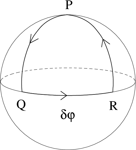
Refer to caption — Figure 1: Path in parameter space starting and ending at P. The duration of the path segments P $\rightarrow$ Q, Q $\rightarrow$ R, and R $\rightarrow$ P is $T_{1}$ , $T_{2}$ , and $T_{3}$ , respectively, as described in Eq. (V.1). $\delta\varphi$ is the opening angle in the equatorial plane. Note that for this path the enclosed solid angle equals $\delta\varphi$ .

For the initial state vector $|\Psi\rangle=\cos(x/2)|0\rangle+e^{-iy}\sin(x/2)|1\rangle$ , the output state of the approximation projected onto the computational space may be written as

	$\displaystyle\bm{\rho}^{a}_{\mathrm{out}}$	$\displaystyle=$	$\displaystyle\bm{u}[\mathcal{C}]\bm{\rho}^{\prime}\bm{u}^{\dagger}[\mathcal{C}],$
	$\displaystyle\bm{\rho}^{\prime}$	$\displaystyle=$	$\displaystyle\left(\begin{array}[]{cc}\frac{1}{2}+\frac{1}{2}\,\cos x&f_{1}\\ f_{1}^{*}&\left(\frac{1}{2}-\frac{1}{2}\cos x\right)f_{2}\end{array}\right),$

where

	$\displaystyle f_{1}$	$\displaystyle=$	$\displaystyle\frac{1}{2}e^{-\frac{1}{4}\Gamma\left(T_{3}+2T_{2}+T_{1}\right)}e^{-iy}\sin x,$		(82)
	$\displaystyle f_{2}$	$\displaystyle=$	$\displaystyle\frac{1}{3}+\frac{2}{3}e^{-\frac{3}{16}\Gamma(T_{3}+T_{1})},$		(83)

and $\bm{u}[\mathcal{C}]$ is the holonomy Eq. (68) in the $\{|0\rangle,|1\rangle\}$ basis. Thus, the output is determined by the holonomy transformation of the $\delta\varphi$ -independent $\bm{\rho}^{\prime}$ . It is worth to point out that this feature is due to the particular choice of parametrization and the chosen loop in parameter space, and not some intrinsic property of the decoherence. Furthermore, in addition to destroying the superpositions between the computational states the decoherence also gives an intensity loss from the computational space. This intensity loss arises as the states corresponding to $\chi_{2}(s)$ , $\chi_{3}(s)$ , and $\chi_{4}(s)$ decoheres into mixed states, as all three of them contain the $a$ state.

As a final observation we note that Eq. (72) can be obtained more or less directly from Eq. (2). We may represent Eq. (2) using an instantaneous orthonormal eigenbasis $\{|\chi_{k}(s)\rangle\}_{k}$ as

\dot{\bm{\rho}}=\bm{M}(s)\bm{\rho},

(84)

where $\bm{M}(s)$ is a $16\times 16$ matrix, and where

\bm{\rho}\equiv\left(\begin{array}[]{c c c c c c c c}\rho_{11}&\rho_{12}&\cdots&\rho_{14}&\rho_{21}&\cdots&\rho_{44}\end{array}\right)^{t}

(85)

with $\rho_{kl}(s)=\langle\chi_{k}(s)|\rho(s)|\chi_{l}(s)\rangle,\ k,l=1,\ldots,4$ . Due to Eq. (7) it follows that Eq. (84) is also obtained if we instead represent Eq. (9) using the $\{|\chi_{k}(0)\rangle\}_{k}$ basis, where we again assume that $U(s)$ is constructed via Eq. (70) with $U_{0}=\hat{1}$ . Equation (11) is obtained by removing couplings from Eq. (9). For the chosen basis, this corresponds to a removal of off-diagonal elements in $\bm{M}(s)$ , such that the new approximate matrix can be arranged in a block diagonal form. Each of these diagonal blocks corresponds to a collection of coupled terms. One block corresponds to the diagonal terms, and there is one block for each collection of off-diagonal terms that couples among themselves, as determined by $g_{klk^{\prime}l^{\prime}}$ . If one is interested in the evolution of a particular collection of coupled terms, then the approximate equation is obtained if one removes those rows and columns from $\bm{M}(s)$ that correspond to terms not included in the collection. In the present example, the matrix $\bm{M}^{a}(s)$ in Eq. (74) is obtained if we use the basis in Eq. (V.1) to represent the exact master equation, and remove those rows and columns from $\bm{M}(s)$ that correspond to the off-diagonal terms.

V.2 Numerical analysis

We compare the approximate solution in Eq. (V.1) with a numerical solution of Eq. (84) in the Hadamard case $\Omega=\pi/4$ by putting $\delta\varphi=\pi/4$ . For the calculation we have used the gauge where the vector potential is well defined at the north pole. We further put $T_{4}=0$ . We distribute the run-time $T$ proportionally to the length of the three circle segments, i.e., $T_{1}=T_{3}=2T/5$ , $T_{2}=T/5$ .

In the numerical treatment of the evolution we decompose the interval $[0,T]$ into subintervals with step size $\Delta t$ , on which $\bm{M}(t)$ is taken to be constant. The resulting approximate evolution is on the form $\bm{\rho}_{K}=\big[\Pi_{k=0}^{K}\exp\bm{(}\Delta t\bm{M}(t_{k})\bm{)}\big]\bm{\rho}_{0}$ . The step size $\Delta t=0.01$ is used. The step size $\Delta t=0.005$ has been tested, without any significant change of the result.

For quantum gates, the relevant error is that at the end-point. This error may contain a contribution in form of an intensity loss out of the computational subspace. To detect this intensity loss, we use the quantities

	$\displaystyle I(T)$	$\displaystyle=$	$\displaystyle 1-{\textrm{Tr}}\big(P\varrho(T)\big),$
	$\displaystyle I^{a}(T)$	$\displaystyle=$	$\displaystyle 1-{\textrm{Tr}}\big(P\varrho^{a}(T)\big)$		(86)

with $P$ the projector onto the computational subspace spanned by $|0\rangle$ and $|1\rangle$ . The error within this subspace is analyzed in terms of the fidelity Uhlmann 1976; Jozsa 1994

	$\displaystyle D(\varrho_{\mathrm{norm}}(T),\varrho^{a}_{\mathrm{norm}}(T))$
	$\displaystyle\equiv{\textrm{Tr}}\sqrt{\sqrt{\varrho_{\mathrm{norm}}(T)}\varrho^{a}_{\mathrm{norm}}(T)\sqrt{\varrho_{\mathrm{norm}}(T)}},$		(87)

where

	$\displaystyle\varrho_{\mathrm{norm}}(T)$	$\displaystyle=$	$\displaystyle\rho_{\mathrm{norm}}(1)=\frac{P\varrho(T)P}{{\textrm{Tr}}\big(P\varrho(T)\big)},$
	$\displaystyle\varrho^{a}_{\mathrm{norm}}(T)$	$\displaystyle=$	$\displaystyle\rho^{a}_{\mathrm{norm}}(1)=\frac{P\varrho^{a}(T)P}{{\textrm{Tr}}\big(P\varrho^{a}(T)\big)},$		(88)

are the normalized outputs of the exact and the approximate evolution, respectively. This normalization may correspond to a post-selection procedure.

In Fig. 2, we show $\langle 1|\varrho(T)|1\rangle$ and $\langle 1|\varrho^{a}(T)|1\rangle$ , for $\Gamma=0,0.01,0.1$ . We have chosen the initial state vector $|\Psi\rangle=\cos(x/2)|0\rangle+e^{-iy}\sin(x/2)|1\rangle$ with $x=\pi/5$ and $y=3\pi/4$ . The corresponding normalized fidelity $D$ is shown in Fig. 3 and the intensity losses $I(T)$ and $I_{a}(T)$ are shown in Fig. 4. These simulations indicate that for this model system the error seems to decrease with increasing run-times $T$ at a rate more or less equal to the ordinary adiabatic approximation in the closed case, independent of the strength $\Gamma$ of the decoherence process. We have confirmed this finding for other input states.

VI Range of applicability

The analysis in Sec. III suggests that, for a given $\Gamma$ , the error bound in Eq. (58) has a minimum for some value of the run-time $T$ . It is quite straightforward to obtain an example of a system where this appears to be the case. One may consider a time-dependent Hamiltonian of the form

H(s)=e^{-isZ}H_{0}e^{isZ},

(89)

where $H_{0}$ and $Z$ are fixed Hermitian operators. The spectrum of this Hamiltonian is fixed, but the eigenbasis rotates. One may consider the master equation

\dot{\rho}=-iT[H(s),\rho]-\Gamma T[A,[A,\rho]],

(90)

where $A$ is a fixed Hermitian operator. The double commutator in the above equation causes decoherence with respect to the eigenbasis of $A$ . We have chosen a four dimensional Hilbert space and have generated $H_{0}$ , $Z$ , and $A$ , as well as the pure initial state, randomly. Figure 5 shows the maximum error in the Hilbert-Schmidt norm $\max_{s\in[0,1]}||\rho(s)-\rho^{a}(s)||$ for various choices of $T$ and $\Gamma$ . As seen in Fig. 5 we indeed seem to have the expected behavior of the approximation. In the ideal case, $\Gamma=0$ , the error appears to go to zero as $T$ increases, while for non-vanishing $\Gamma$ there seems to be a minimum error.

However, the error does not always seem to behave in this manner. In the example presented in Sec. V.2 there is no trace of this minimum error. Rather the error seems to vanish for large $T$ for any value of $\Gamma$ . In other words, the error bounds derived in Sec. III appears to be unnecessarily pessimistic in some cases. We here put forward some reasons why this may be the case.

One aspect is the question of which error to consider. In Sec. III we considered the maximum deviation between the exact and approximate solution during the whole evolution, while in Sec. V.2, the relevant error was taken at the end of the evolution. In some cases the maximum deviation need not occur at the end of the evolution, which may cause the “end point error” to be smaller than the maximum deviation. One may also note that Sec. V.2 focused on one single diagonal term of the total density operator and that the error for this part may be smaller than the total error.

Another reason for the approximation to be accurate under wider conditions is if the dissipator $D_{s}$ is such that it does not couple off-diagonal terms to diagonal terms, or off-diagonal terms to other off-diagonal terms. Under such conditions the dissipator is unaffected by the approximation and it seems reasonable that the approximation should have a wider range of applicability. However, this cannot be the sole reason, as is indicated by the results in Sec. V.2, since the dissipator used (i.e., decoherence with pointer state $a$ ) does belong to the class of dissipators that do couple the diagonal and off-diagonal terms. Suppose, however, that the evolution is such that the magnitude of the off-diagonal terms tends to decrease with increasing run-times. For example, this may occur if a decoherence or relaxation process acts suitably in relation to the instantaneous eigenspaces. Consider the diagonal terms: even if there would be a coupling to the off-diagonal terms, the importance of this coupling naturally diminishes if the off-diagonal terms tends to decrease in magnitude. If the open system process is such that it tends to suppress the off-diagonal terms, it thus seems reasonable to expect that the approximate equation should be accurate at large run-times. This reduction of off-diagonal terms reasonably should be more relevant for the end point error than for the maximum deviation. Another reason for the end-point error to vanish is if the approximate and exact equations have a common asymptotic state.

There is clearly room for further investigations of when and why the present approximation is accurate beyond the joint limit of slow change and weak open system effects.

VII Conclusions

We present an adiabatic approximation scheme for weakly open systems. Contrary to the adiabatic approximation for closed systems, the presence of open system effects introduces a coupling between the instantaneous eigenspaces of the time-dependent, possibly degenerate, Hamiltonian. We show that the present approximation can be obtained as a slow-change weak open-system limit, in the sense that the time scale inversely proportional to the strength of the open system effect puts an upper limit on the run-time. In the ideal case of closed systems this limiting time scale becomes infinite, and the ordinary adiabatic approximation Messiah 1962 is retained.

We demonstrate the approximation scheme for a non-Abelian holonomic implementation of a Hadamard gate, exposed to a decoherence process. We compare the approximation with numerically obtained solutions of the exact master equation. These calculations indicate that the error between the approximate and the exact evolution decreases with increasing run-time at a rate more or less independent of the strength of the decoherence process. This result suggests that the approximation scheme may have a wider range of applicability than the weak open-system limit.

References

Messiah (1962) A. Messiah, Quantum Mechanics (North-Holland, Amsterdam, 1962), Vol. 2.
Zanardi and Rasetti (1999) P. Zanardi and M. Rasetti, Phys. Lett. A 264, 94 (1999).
Farhi et al. (2000) E. Farhi, J. Goldstone, S. Gutmann, and M. Sipser, eprint quant-ph/0001106.
Farhi et al. (2001) E. Farhi, J. Goldstone, S. Gutmann, J. Lapan, A. Lundgren, and D. Preda, Science 292, 472 (2001).
Romero et al. (2002) K. M. F. Romero, A. C. A. Pinto, and M. T. Thomaz, Physica A 307, 142 (2002).
Pinto et al. (2002) A. C. A. Pinto, K. M. F. Romero, and M. T. Thomaz, Physica A 311, 169 (2002).
Wilczek and Zee (1984) F. Wilczek and A. Zee, Phys. Rev. Lett 52, 2111 (1984).
Sarandy and Lidar (2005a) M. S. Sarandy and D. A. Lidar, Phys. Rev. A 71, 012331 (2005a).
Sarandy and Lidar (2005) M. S. Sarandy and D. A. Lidar, eprint quant-ph/0502014.
(10) J. Åberg, D. Kult, and E. Sjöqvist, Phys. Rev. A 71, 060312(R) (2005a).
(11) By putting $\Gamma=0$ in Eq. (4) we obtain the Schrödinger equation $|\dot{\psi}\rangle=-i[TH(s)+Q(s)]|\psi\rangle$ . If $H(s)$ is nondegenerate with orthonormal eigenbasis $\{|\chi_{k}(s)\rangle\}_{k}$ , then we may write $|\psi(s)\rangle=\sum_{k}c_{k}(s)|\chi_{k}(s)\rangle$ . The resulting equations for the coefficients $c_{k}$ become $\dot{c}_{k}(s)=[-iTE_{k}(s)+\langle\dot{\chi}_{k}(s)|\chi_{k}(s)\rangle]c_{k}(s)$ .
Marsden and Hoffman (1987) J. E. Marsden and M. J. Hoffman, Basic Complex Analysis (Freeman, New York, 1987).
Churchill (1963) R. V. Churchill, Fourier Series and Boundary Value Problems (McGraw-Hill, New York, 1963).
Rellich (1969) F. Rellich, Perturbation Theory of Eigenvalue Problems (Gordon and Breach, New York, 1969).
Amann (1990) H. Amann, de Gruyter Studies in Mathematics. Ordinary Differential Equations (Walter de Gruyter, Berlin, 1990), Vol. 13.
(16) M. Reed and B. Simon, Methods of Modern Mathematical Physics IV: Analysis of Operators (Academic Press, New York, 1978).
(17) Note that a similar breakdown of adiabaticity after a finite time has previously been reported in Ref. Sarandy and Lidar 2005a and has been further discussed in Ref. Sarandy and Lidar 2005.
Lindblad (1976) G. Lindblad, Comm. Math. Phys. 48, 119 (1976).
Gorini et al. (1976) V. Gorini, A. Kossakowski, and E. C. G. Sudarshan, J. Math. Phys. 17, 821 (1976).
Kraus (1983) K. Kraus, States, Effects, and Operations, Lecture Notes in Physics Vol. 190 (Springer, Berlin, 1983).
Alicki and Lendi (1987) R. Alicki and K. Lendi, Quantum Dynamical Semigroups and Applications, Lecture Notes in Physics Vol. 286 (Springer, Berlin, 1987).
Lendi (1986) K. Lendi, Phys. Rev. A 33, 3358 (1986).
Wilkie (2000) J. Wilkie, Phys. Rev. E 62, 8808 (2000).
Breuer (2004) H.-P. Breuer, Phys. Rev. A 70, 012106 (2004).
Unanyan et al. (1999) R. G. Unanyan, B. W. Shore, and K. Bergmann, Phys. Rev. A 59, 2910 (1999).
Duan et al. (2001) L. M. Duan, J. I. Cirac, and P. Zoller, Science 292, 1695 (2001).
Faoro et al. (2003) L. Faoro, J. Siewert, and R. Fazio, Phys. Rev. Lett. 90, 028301 (2003).
Solinas et al. (2003) P. Solinas, P. Zanardi, N. Zanghì, and F. Rossi, Phys. Rev. A 67, 062315 (2003).
Recati et al. (2002) A. Recati, T. Calarco, P. Zanardi, J. I. Cirac, and P. Zoller, Phys. Rev. A 66, 032309 (2002).
Uhlmann (1976) A. Uhlmann, Rep. Math. Phys 9, 273 (1976).
Jozsa (1994) R. Jozsa, J. Mod. Opt. 41, 2315 (1994).

	$\displaystyle\|\|f_{d}(s,\sigma)-f_{d}(s,\sigma^{\prime})\|\|$
	$\displaystyle\leq\sum_{l}\|\|P_{l}(0)[Z_{l}(s),P_{l}(0)(\sigma-\sigma^{\prime})P_{l}(0)]P_{l}(0)\|\|$
	$\displaystyle\quad+\Gamma T\sum_{kl}\|\|P_{l}(0)D_{s}\!\bm{(}P_{k}(0)(\sigma-\sigma^{\prime})P_{k}(0)\bm{)}P_{l}(0)\|\|$
	$\displaystyle\leq(F^{(d)}+G^{(d)}\Gamma T)\|\|\sigma-\sigma^{\prime}\|\|,$		(36)

$\displaystyle\|\chi_{1}(s)\rangle$	$\displaystyle=$	$\displaystyle\cos\varphi(s)\|0\rangle-\sin\varphi(s)\|1\rangle,$
$\displaystyle\|\chi_{2}(s)\rangle$	$\displaystyle=$	$\displaystyle\sin\varphi(s)\cos\theta(s)\|0\rangle+\cos\varphi(s)\cos\theta(s)\|1\rangle-\sin\theta(s)\|a\rangle,$
$\displaystyle\|\chi_{3}(s)\rangle$	$\displaystyle=$	$\displaystyle\frac{1}{\sqrt{2}}\Big(\sin\varphi(s)\sin\theta(s)\|0\rangle+\cos\varphi(s)\sin\theta(s)\|1\rangle+\cos\theta(s)\|a\rangle+\|e\rangle\Big),$
$\displaystyle\|\chi_{4}(s)\rangle$	$\displaystyle=$	$\displaystyle\frac{1}{\sqrt{2}}\Big(\sin\varphi(s)\sin\theta(s)\|0\rangle+\cos\varphi(s)\sin\theta(s)\|1\rangle+\cos\theta(s)\|a\rangle-\|e\rangle\Big),$	(73)