跳到论文正文
W Papers独立论文阅读器 arXiv:quant-ph/0503013 论文正文 计算阅读时间 · 0%
引用这篇论文根据当前论文元数据生成,正式投稿前建议核对。


License: Assumed arXiv.org perpetual non-exclusive license
arXiv:quant-ph/0503013v1 [quant-ph] 01 Mar 2005

Entanglement Distillation Protocols and Number Theory

H. Bombin and M.A. Martin-Delgado Affiliation:  Departamento de Física Teórica I, Universidad Complutense, 28040. Madrid, Spain.
Abstract

We show that the analysis of entanglement distillation protocols for qudits of arbitrary dimension DD benefits from applying basic concepts from number theory, since the set 𝐙Dn\mathbf{Z}_{D}^{n} associated to Bell diagonal states is a module rather than a vector space. We find that a partition of 𝐙Dn\mathbf{Z}_{D}^{n} into divisor classes characterizes the invariant properties of mixed Bell diagonal states under local permutations. We construct a very general class of recursion protocols by means of unitary operations implementing these local permutations. We study these distillation protocols depending on whether we use twirling operations in the intermediate steps or not, and we study them both analitically and numerically with Monte Carlo methods. In the absence of twirling operations, we construct extensions of the quantum privacy algorithms valid for secure communications with qudits of any dimension DD. When DD is a prime number, we show that distillation protocols are optimal both qualitatively and quantitatively.

pacs
03.67.-a, 03.67.Lx

I Introduction

Quantum Information Theory (QIT) revolves around the concept of entanglement review1, review2, book, rmp. It is the product of combining the superposition principle of Quantum Mechanics with multipartite systems – described by tensor product of Hilbert spaces. Entanglement is central to transmiting information in a quantum communication protocol or processing information in a quantum computation. There are two basic open problems in the study of entanglement: separability and distillability. Separability is concerned with two questions, namely, whether a quantum state is factorizable and if not, how much entanglement it contains. These questions are of great importance even in practice since entanglement amounts to interaction between two or more parties, and thus it demands more resources to establish an entangled state than a factorized one.

Likewise, distillability bennett1, super, qpa, chiara1, horodeckis, permutations, beyond is concerned with two questions: whether a quantum state is distillable, and if it is, how to devise an explicit protocol to extract entanglement out of the initial low entangled state. The main focus of our paper is on the construction of distillation protocols, rather than a direct analysis of the distillability issue.

The study of distillation protocols for qudits is justified since it is known that for mixed states of dimension higher than 2×2,2×32\times 2,2\times 3, it is neither known a complete critierion for separability nor for distillability horodeckis.

Separability and distillability are interconnected. Entanglement of a mixed state is a necessary condition for being distillable. However, it was quite a surprise to find that there exist states that though entangled, they cannot be distilled. They are the bound entangled states that are characterized by being PPT (Positive Partial Transposition) entangled states pavel, bound1, bound2. This situation soon raised the question of whether Non-PPT states were all distillable. Although there is not a conclusive answer, yet there is strong evidence that this is neither the case since Werner states which are finite-nn undistillable have been found evidence1, evidence2.

In this paper we study entanglement distillation protocols for qudits using the recursion method bennett1, super. The mixed states to be distilled are diagonal Bell states of qudits, but they do not need to be tensor product of pairs of Bell states. Moreover, we can also distill non-diagonal states.

We make significative progress in the understanding of these protocols and find new efficient variants of them by using number theory. This number theory enters in the properties of the module 𝐙Dn\mathbf{Z}_{D}^{n} that appears in the labelling of the Bell diagonal sates of qudits. Local permutations acting on these states by means of unitary operations serve to construct generalized distillation protocols permutations. As a byproduct, we also introduce heterotropic states (38) as the invariant states under the group of local permutations.

As a result of this study, we find that qudit states with dimension DD a prime number are qualitatively and quantitatively the best choices for quantum distillation protocols based on the recursion method. Qualitatively, since we show that for DD not a prime number there appear disturbing attractor points in the space of fidelity parameters that deviate the distillation process from the desired fixed point that represents the maximally entangled state. This phenomenon is absent when DD is a prime number and 𝐙Dn\mathbf{Z}_{D}^{n} becomes a vector space. Quantitatively, since we propose distillation protocols that when DD is a prime number, they distill all states with fidelity bigger than 1D\frac{1}{D} without resorting to twirling operations.

We hereby summarize briefly some of our main results:

i/ We proof that the group of local permutations for qudits of arbitrary dimension DD is the semidirect product of the group of translations and simplectic transformations. This structure plays an important role in the distillation protocols for qudits.

ii/ We simplify the problem of finding the best distillation protocol to that of finding the best set of coefficients of a certain polinomial constrained to the existence of a suitable vector space.

iii/ We introduce the concept of joint performance parameter η\eta (65) that allows us the comparison of distillation protocols with different values of fidelity, probability of success and number of Bell pairs used altogether. It is a figure of merit for low fidelity states above the distillation threshold where the recursion method is specially suited for distillation, prior to switching a hashing or breeding method.

iv/ We analyze several distillation protocols assisted with twirling operations as the dimension DD of qudits vary. We find that the best performance according to η\eta is not achieved for qubits (D=2D=2), but for qutrits (D=3D=3) and n=3n=3 input pairs of Bell states as shown in Fig. 1 and Fig. 2. We also find that it is not possible to improve η\eta by indefinitely increasing the number of input pairs nn.

v/ We propose a distillation protocol without resorting to twirling operations for n=4n=4 input Bell states and m=2m=2 output Bell states that is iterative and its yield is greatly improved: about four orders of magnitude with respect to the protocols based on twirling, even for states quite near the fixed point. This is shown in Fig. 5.

vi/ We propose and study an extension of the Quantum Privacy Amplification protocols qpa that work for arbitrary dimension DD.

vii/ We find indications of the existence of non-distillable NPPT states by studying the distillation capacities of protocols for several values of DD, as shown in Fig. 7.

This paper is organized as follows: In order to facilitate the reading and exposition of our results, we present the proofs of our theorems and technicalities of the numerical methods in independent appendices. Sect. II deals with the basic properties of diagonal Bell states for qudits and introduce a partition of the module 𝐙Dn\mathbf{Z}_{D}^{n}. Sect. III treats the group of local permutations acting on qudits in diagonal Bell states. Sect IV describes the group of local permutations and the twirling operations associated with it. We characterize states that are invariant under these operations as heterotropic states. In Sect. V we present all our distillation protocols based on local permutations of qudits in diagonal Bell states, both with and without resorting to twirling operations. To this end, we make extensive use of the theoretical results found in previous sections and devise numerical methods to analyse efficiently the properties of the proposed distillation protocols as different parameters such as DD, FF, n,mn,m etc. vary. Sect. VI is devoted to conclusions and future prospects.

II Basic Properties of Diagonal Bell States for Qudits

II.1 Bell States Basic Notation

The quantum systems we are going to consider are qudits, which are described by a Hilbert space of dimension D≥2D\geq 2, and finite. The elements of a given orthogonal basis can be denoted |x⟩|x\rangle with x=0,…,D−1x=0,\dots,D-1. This set of numbers is naturally identified with the elements of the set modulus

𝐙D:=𝐙/D​𝐙,\mathbf{Z}_{D}:=\mathbf{Z}/D\mathbf{Z}, (1)

and we shall informally use them as if they belonged to 𝐙D\mathbf{Z}_{D}. In general, whenever an element of 𝐙D\mathbf{Z}_{D} appears in an expression, any integer in that expression must be understood to be mapped to 𝐙D\mathbf{Z}_{D}.

We consider two separated parties, Alice and Bob, each of them owning one of these systems. The entire Hilbert space then is ℋ=ℋA⊗ℋB\mathcal{H}=\mathcal{H}_{A}\otimes\mathcal{H}_{B}. A mixed state of the whole system is called separable when it can be expressed as a convex sum of product states werner:

ρ=∑ipi​|ei⟩​⟨ei|⊗|fi⟩​⟨fi|,|ei⟩∈ℋA,|fi⟩∈ℋB;\rho=\sum_{i}p_{i}|e_{i}\rangle\langle e_{i}|\otimes|f_{i}\rangle\langle f_{i}|,\ \ |e_{i}\rangle\in\mathcal{H}_{A},\,|f_{i}\rangle\in\mathcal{H}_{B}; (2)

A state which is not separable is said to be entangled.

Elements of the computational basis of a pair of qudits shared by Alice and Bob are denoted as

|i​j⟩:=|i⟩⊗|j⟩,i,j∈𝐙D.|i\;j\rangle:=|i\rangle\otimes|j\rangle,\qquad i,j\in\mathbf{Z}_{D}. (3)

To shorthen the notation, it is convenient to introduce the symbols

𝒮𝑘:=1D∑k∈𝐙D,δ(k):=Dδk,0,φ(k):=e2​π​iD​k,\displaystyle{{\underset{\text{\raisebox{-0.60275pt}{$k$}}}{\raisebox{-2.58334pt}{\text{\LARGE$\mathcal{S}$}}}}}:=\frac{1}{\sqrt{D}}{\sum_{k\in\mathbf{Z}_{D}}},\quad\delta(k):=\sqrt{D}\delta_{k,0},\quad\varphi(k):={\rm e}^{\frac{2\pi{\rm i}}{D}k}, (4)

chosen so that 𝒮k​φ​(i​k)=δ⁡(i){\text{\Large$\mathcal{S}$}}_{k}\,\varphi(ik)=\delta(i) and 𝒮k​δ​(i−k)​f​(k)=f⁡(i){\text{\Large$\mathcal{S}$}}_{k}\,\delta(i-k)f(k)=f(i) (i∈𝐙D)(i\in\mathbf{Z}_{D}). Bell states are defined as gisin1, gisin2, mamd1, mamd2

|i​j⟩​ℬ:=𝒮𝑘​φ​(k​i)​|k​k−j⟩i,j∈𝐙D.|i\;j\rangle\!\text{\hskip 0.86108pt}\text{\raisebox{-2.15277pt}{${\scriptscriptstyle{\mathcal{B}}}$}}:={{\underset{\text{\raisebox{-0.60275pt}{$k$}}}{\raisebox{-2.58334pt}{\text{\LARGE$\mathcal{S}$}}}}}\varphi(ki)|k\;k-j\rangle\qquad i,j\in\mathbf{Z}_{D}. (5)

Bell states are an example of maximally entangled states. In fact, any maximally entangled state can be identified with the |0 0⟩​ℬ|0\;0\rangle\!\text{\hskip 0.86108pt}\text{\raisebox{-2.15277pt}{${\scriptscriptstyle{\mathcal{B}}}$}} state by suitably choosing the computational basis of each of the qudits, due to the Schmidt decomposition.

The fidelity of a mixed state ρ\rho is defined as

F:=maxΨ⁡⟨Ψ|ρ|Ψ⟩,F:=\max_{\Psi}\langle\Psi|\rho|\Psi\rangle, (6)

where the maximum is taken over the set of maximally entangled states. The aim of distillation protocols is to get maximally entangled pairs (fidelity one) by means of local operations and classical communication (LOCC), starting with entangled states of fidelity lower than one. Because of the previous comment, we will always suppose, without lose of generality, that the initial fidelity of the states to be distilled is equal to ℬ​ ​⟨0 0|ρ|0 0⟩​ℬ\text{\raisebox{-2.15277pt}{${\scriptscriptstyle{\mathcal{B}}}$}}\!\text{\hskip 1.07639pt}\langle 0\;0|\rho|0\;0\rangle\!\text{\hskip 0.86108pt}\text{\raisebox{-2.15277pt}{${\scriptscriptstyle{\mathcal{B}}}$}}, and the aim of our protocols will be to obtain distilled states as close as possible to this Bell state.

Of special interest are the mixtures of perfectly entangled states and white noise, known as isotropic states:

ρiso:=F⁡|0 0⟩​ℬ​ ​⟨0 0|+1−FD2−1​(1−|0 0⟩​ℬ​ ​⟨0 0|),\rho_{\rm iso}:=F\>|0\;0\rangle\!\text{\hskip 0.86108pt}\text{\raisebox{-2.15277pt}{${\scriptscriptstyle{\mathcal{B}}}$}}\!\text{\hskip 1.07639pt}\langle 0\;0|+\frac{1-F}{D^{2}-1}\>\bigl(1-|0\;0\rangle\!\text{\hskip 0.86108pt}\text{\raisebox{-2.15277pt}{${\scriptscriptstyle{\mathcal{B}}}$}}\!\text{\hskip 1.07639pt}\langle 0\;0|\bigr), (7)

where FF is the fidelity of the state. These states are known to be entangled and distillable iff F>1DF>\frac{1}{D} horodeckis.

The main interest of these states comes not only from their physical meaning, but also from the possibility of transforming any state in an isotropic one through a twirling operation. In general, the twirling consists in a random application of the elements of a certain group of unitary operations, say 𝒰\mathcal{U}, to each of the systems in an ensemble. Namely, its action is

T𝒰​(ρ):=∫𝒰d​U​U​ρ​U†.T_{\mathcal{U}}(\rho):=\int_{\mathcal{U}}dU\,U\rho\,U^{\dagger}. (8)

The result of such an operator must be a sum over the states invariant under the action of the group. In the case of isotropic states, a suitable election is the set of transformations of the form U⊗U∗U\otimes U^{\ast}.

When managing multiple shared pairs, vector notation is necessary; 𝐤∈𝐙Dn\boldsymbol{\mathrm{k}}\in\mathbf{Z}_{D}^{n} stands for 𝐤=(k1,…,kn),ki∈𝐙D\boldsymbol{\mathrm{k}}=(k_{1},\dots,k_{n}),k_{i}\in\mathbf{Z}_{D}. Scalar product will be employed with its usual meaning. The generalization of the previous expressions is straightforward:

𝒮𝐤:=𝒮k1​⋯​𝒮kn,δ⁡(𝐤):=δ⁡(k1)​⋯​δ​(kn).{{\underset{\text{\raisebox{-0.60275pt}{$\boldsymbol{\mathrm{k}}$}}}{\raisebox{-2.58334pt}{\text{\LARGE$\mathcal{S}$}}}}}:={{\underset{\text{\raisebox{-0.60275pt}{$k_{1}$}}}{\raisebox{-2.58334pt}{\text{\LARGE$\mathcal{S}$}}}}}\dotsi{{\underset{\text{\raisebox{-0.60275pt}{$k_{n}$}}}{\raisebox{-2.58334pt}{\text{\LARGE$\mathcal{S}$}}}}},\quad\delta(\boldsymbol{\mathrm{k}}):=\delta(k_{1})\dotsi\delta(k_{n}). (9)

Again, 𝒮𝐤​φ​(𝐢⋅𝐤)=δ⁡(𝐢){\text{\Large$\mathcal{S}$}}_{\boldsymbol{\mathrm{k}}}\,\varphi(\boldsymbol{\mathrm{i}}\cdot\boldsymbol{\mathrm{k}})=\delta(\boldsymbol{\mathrm{i}}) for any 𝐢∈𝐙Dn\boldsymbol{\mathrm{i}}\in\mathbf{Z}_{D}^{n}. The computational basis and the Bell basis are:

|𝐢​𝐣⟩\displaystyle|\boldsymbol{\mathrm{i}}\;\boldsymbol{\mathrm{j}}\rangle :=⨂k=1𝑛​|ik​jk⟩,\displaystyle:=\overset{n}{\bigotimes_{k=1}}\,|i_{k}\;j_{k}\rangle,
|𝐢​𝐣⟩​ℬ\displaystyle|\boldsymbol{\mathrm{i}}\;\boldsymbol{\mathrm{j}}\rangle\!\text{\hskip 0.86108pt}\text{\raisebox{-2.15277pt}{${\scriptscriptstyle{\mathcal{B}}}$}} :=⨂k=1𝑛​|ik​jk⟩​ℬ=𝒮𝐤​φ​(𝐢⋅𝐤)​|𝐤​𝐤−𝐣⟩,\displaystyle:=\overset{n}{\bigotimes_{k=1}}\,|i_{k}\;j_{k}\rangle\!\text{\hskip 0.86108pt}\text{\raisebox{-2.15277pt}{${\scriptscriptstyle{\mathcal{B}}}$}}={{\underset{\text{\raisebox{-0.60275pt}{$\boldsymbol{\mathrm{k}}$}}}{\raisebox{-2.58334pt}{\text{\LARGE$\mathcal{S}$}}}}}\varphi(\boldsymbol{\mathrm{i}}\cdot\boldsymbol{\mathrm{k}})|\boldsymbol{\mathrm{k}}\;\boldsymbol{\mathrm{k}}-\boldsymbol{\mathrm{j}}\rangle, (10)

with 𝐢,𝐣∈𝐙Dn\boldsymbol{\mathrm{i}},\boldsymbol{\mathrm{j}}\in\mathbf{Z}_{D}^{n}. In order to simplify the notation, sometimes we will work with vectors over 𝐙D2​n\mathbf{Z}_{D}^{2n} and write states as |𝐱⟩|\boldsymbol{\mathrm{x}}\rangle in the place of |𝐢​𝐣⟩|\boldsymbol{\mathrm{i}}\;\boldsymbol{\mathrm{j}}\rangle, with

𝐱:=(i1,…,in,j1,…,jn).\boldsymbol{\mathrm{x}}:=(i_{1},\dots,i_{n},j_{1},\dots,j_{n}). (11)

II.2 A Partition of 𝐙Dn\mathbf{Z}_{D}^{n} with Divisor Classes

In general, 𝐙D\mathbf{Z}_{D} is not a field and thus 𝐙Dn\mathbf{Z}_{D}^{n} is not a vector space, but a module. We can still make use of some properties associated to vector spaces and so we will abuse a bit of the term vector. For a detailed exposition see appendix A, but it is enough to know the following. The usual definition of linear independence makes sense, as one can demonstrate that any linearly independent set of vectors can be extended to a complete base and also that a square matrix composed by such a set is invertible. A subspace is defined to be the set of linear combinations of a linearly independent set, and its dimension is the cardinality of these set of generators. Orthogonality poses no problem, since the set orthogonal to a subspace is a subspace, and it has the expected dimension.

Working with this pseudo-vector space 𝐙Dn\mathbf{Z}_{D}^{n} requires care. Some vectors can be taken to the null vector by multiplying them by a non-zero number. For example, for D=4D=4 we have 2⋅(0,2)=(0,0)2\cdot(0,2)=(0,0). In order to classify this anomalous vectors, consider the set of divisors of D:

div(D):={d∈𝐍:d|D}.\mathrm{div}(D):=\{\,d\in\mathbf{N}:d|D\,\}. (12)

This set inherits the ordering of 𝐍\mathbf{N}, and we shall use this property to introduce a suitable gcd\gcd function in 𝐙D\mathbf{Z}_{D}:

Definition II.1

For every S⊂𝐙DS\subset\mathbf{Z}_{D} we define the greatest common divisor of SS, or gcd⁡(S)\gcd(S), to be the greatest d∈div⁡(D)d\in\mathrm{div}(D) such that Dd​s=0\frac{D}{d}s=0, ∀s∈S\forall\,s\in S.

The nomenclature was chosen because for any d∈div⁡(D)d\in\mathrm{div}(D) and x∈𝐙x\in\mathbf{Z} we have

d|x⇔D|Dd​x⇔Dd​x=0(modD),d|x\iff D|\frac{D}{d}x\iff\frac{D}{d}x=0\pmod{D}, (13)

and then for any set of integers XX

gcd(X¯)=max{d∈div(D):d|x∀x∈X},\gcd(\overline{X})=\max\{\,d\in\mathrm{div}(D):d|x\>\forall\,x\in X\,\}, (14)

where X¯\overline{X} is the corresponding set in 𝐙D\mathbf{Z}_{D}.

DD 22 3 4 5 6
ϕ1​(D)\phi_{1}(D) 1 2 2 4 2
ϕ2​(D)\phi_{2}(D) 3 8 12 24 24
ϕ3​(D)\phi_{3}(D) 7 26 56 124 182
Table 1: Values of the generalized Euler’s totient function ϕn​(D)\phi_{n}(D) for several qudit dimensions DD.
D 2 3 4 5 6
♯​𝒫S​(D,1)\sharp\mathcal{P}_{\scriptscriptstyle{\mathrm{S}}}(D,1) 6 24 48 120 144
♯​𝒫S​(D,2)\sharp\mathcal{P}_{\scriptscriptstyle{\mathrm{S}}}(D,2) 720 51,840 737,280 9.36⋅1069.36\cdot 10^{6} ∼3.7⋅107\sim 3.7\cdot 10^{7}
♯​𝒫S​(D,3)\sharp\mathcal{P}_{\scriptscriptstyle{\mathrm{S}}}(D,3) 1,451,520 ∼9.2⋅109\sim 9.2\cdot 10^{9} ∼3.0⋅1012\sim 3.0\cdot 10^{12} ∼9.1⋅1013\sim 9.1\cdot 10^{13} ∼1.3⋅1016\sim 1.3\cdot 10^{16}
Table 2: Values of the number of elements of the group 𝒫S​(D,n)\mathcal{P}_{\scriptscriptstyle{\mathrm{S}}}(D,n) for several qudit dimensions DD.

Vectors over 𝐙D\mathbf{Z}_{D} are n-tuples of elements in 𝐙D\mathbf{Z}_{D}, and so we extend the gcd\gcd function to act over 𝐙Dn\mathbf{Z}_{D}^{n} in the natural way, that is, if 𝐯=(v1,…​vn)\boldsymbol{\mathrm{v}}=(v_{1},\dots\,v_{n}), gcd⁡(𝐯):=gcd⁡({v1,…,vn})\gcd(\boldsymbol{\mathrm{v}}):=\gcd(\{v_{1},\dots,v_{n}\}). Now we can consider an equivalence relation in 𝐙Dn\mathbf{Z}_{D}^{n} governed by the equality under the gcd\gcd function. The corresponding partition consists in the sets:

Cd​(D,n):={𝐯∈𝐙Dn:gcd⁡(𝐯)=d},d∈div⁡(D)C_{d}(D,n):=\{\,\boldsymbol{\mathrm{v}}\in\mathbf{Z}_{D}^{n}:\gcd(\boldsymbol{\mathrm{v}})=d\,\},\ d\in\mathrm{div}(D) (15)

The most important of these sets is C1​(D,n)C_{1}(D,n), since it contains those vectors 𝐯\boldsymbol{\mathrm{v}} for with {𝐯}\{\boldsymbol{\mathrm{v}}\} is linearly independent. Later we will need its cardinality when considering properties of local unitary operators acting on diagonal Bell states. Thus, it is useful to define:

ϕn​(D):={1if D=1♯​C1​(D,n)if D>1\phi_{n}(D):=\begin{cases}1&\text{if $D=1$}\\ \sharp C_{1}(D,n)&\text{if $D>1$}\end{cases} (16)

For the particular case of n=1n=1, ϕ1​(x)\phi_{1}(x) corresponds to Euler’s totient ϕ\phi-function Euler. Euler’s ϕ\phi-function appears naturally in number theory since it gives for a natural number nn, the cardinality of the set {m=1,…,n−1:gcd(m,n)=1}\{\,m=1,\dots,n-1:\gcd(m,n)=1\,\}. That is, ϕ1​(n)\phi_{1}(n) is the total number of coprime integers (or totatives) below or equal to nn. For example, there are eight totatives of 24, namely, {1,5,7,11,13,17,19,23}\{1,5,7,11,13,17,19,23\}, thus ϕ1​(24)=8\phi_{1}(24)=8. For n≠1n\neq 1, we have therefore introduced a generalization of Euler’s totient function for elements in 𝐙Dn\mathbf{Z}_{D}^{n}. The following lemma gives us how to compute the cardinalities of the sets Cd​(D,n)C_{d}(D,n), which shall naturally arise in our analysis of distillation protocols.

Lemma II.2

For every n∈𝐍n\in\mathbf{N}, D∈𝐍−{1}D\in\mathbf{N}-\{1\} and d∈div⁡(D)d\in\mathrm{div}(D):

  1. 1.
    ϕn​(D)=Dn​∏p|Dp​primepn−1pn\phi_{n}(D)=D^{n}\prod_{p|D\atop p\>\mathrm{prime}}\frac{p^{n}-1}{p^{n}} (17)
  2. 2.
    ♯​Cd​(D,n)=ϕn​(Dd)\sharp C_{d}(D,n)=\phi_{n}(\frac{D}{d}) (18)
  3. 3.
    ∑d′∈div⁡(D)ϕn​(d′)=Dn\sum_{d^{\prime}\in\mathrm{div}(D)}\phi_{n}(d^{\prime})=D^{n} (19)

The proof of this lemma can be found in appendix B. As an illustration, we list several values of ϕn​(D)\phi_{n}(D) in Table 1.

III The group of local permutations

The main constraint Alice and Bob have to face when they intend to distill qudits is that they can perform only local operations. If we consider only unitary operations, we are led to the group 𝒰loc\mathcal{U}_{\scriptscriptstyle{\mathrm{loc}}} of local unitary operations. Its elements are all of the form

U=UA⊗UB.U=U_{\mathrm{A}}\otimes U_{\mathrm{B}}. (20)

In this section we shall study the subgroup 𝒰B​loc\mathcal{U}_{\scriptscriptstyle{\mathrm{B\,loc}}}, defined as the group of local unitary operations which are closed over the space of Bell diagonal states, that is, states of the form

ρ(n)=∑𝐱∈𝐙D2​np𝐱(n)​|𝐱⟩​ℬ​ ​⟨𝐱|,\rho^{\scriptscriptstyle(n)}=\sum_{\boldsymbol{\mathrm{x}}\in\mathbf{Z}_{D}^{2n}}p^{\scriptscriptstyle(n)}_{\boldsymbol{\mathrm{x}}}\,|\boldsymbol{\mathrm{x}}\rangle\!\text{\hskip 0.86108pt}\text{\raisebox{-2.15277pt}{${\scriptscriptstyle{\mathcal{B}}}$}}\!\text{\hskip 1.07639pt}\langle\boldsymbol{\mathrm{x}}|, (21)

where the label (n)(n) is a reminder that we are considering states of nn pairs of qudits. The aim is to use the acquired knowledge to devise distillation protocols specially suited for these states.

More specifically, we analyze the group 𝒰B​loc​(D,n)\mathcal{U}_{\scriptscriptstyle{\mathrm{B\,loc}}}(D,n) of local unitary operators over the space spanned by the tensor product of nn pairs of qudits of dimension DD for which the image of a Bell diagonal state is another Bell diagonal state. The first we notice is that the result of applying such an operator over a pure Bell state is another Bell state (it cannot be the convex sum of several Bell states because it must remain pure). Since the mapping of Bell states must be one to one, the action of any U∈𝒰B​loc​(D,n)U\in\mathcal{U}_{\scriptscriptstyle{\mathrm{B\,loc}}}(D,n) involves a permutation of the Bell states:

U​ρ​U†=∑𝐱∈𝐙D2​np𝐱(n)​|π⁡(𝐱)⟩​ℬ​ ​⟨π⁡(𝐱)|,U\rho\,U^{\dagger}=\sum_{\boldsymbol{\mathrm{x}}\in\mathbf{Z}_{D}^{2n}}p^{\scriptscriptstyle(n)}_{\boldsymbol{\mathrm{x}}}\,|\pi(\boldsymbol{\mathrm{x}})\rangle\!\text{\hskip 0.86108pt}\text{\raisebox{-2.15277pt}{${\scriptscriptstyle{\mathcal{B}}}$}}\!\text{\hskip 1.07639pt}\langle\pi(\boldsymbol{\mathrm{x}})|, (22)

where π:𝐙D2​n→𝐙D2​n\pi:\mathbf{Z}_{D}^{2n}\rightarrow\mathbf{Z}_{D}^{2n} is a permutation. So we introduce 𝒫loc​(D,n)\mathcal{P}_{\scriptscriptstyle{\mathrm{loc}}}(D,n), the group of local permutations, as the set of permutations over 𝐙D2​n\mathbf{Z}_{D}^{2n} implementable over Bell states by local (unitary) means.

Before stating the main result of this section, we shall define several groups. Consider the family of unitary operators u𝐱u_{\boldsymbol{\mathrm{x}}} (𝐱∈𝐙D2​n\boldsymbol{\mathrm{x}}\in\mathbf{Z}_{D}^{2n}) over Bob’s part of the system such that by definition

1⊗u𝐱∗​|𝟎⟩​ℬ:=|𝐱⟩​ℬ,1\otimes u_{\boldsymbol{\mathrm{x}}}^{\ast}\,|\boldsymbol{\mathrm{0}}\rangle\!\text{\hskip 0.86108pt}\text{\raisebox{-2.15277pt}{${\scriptscriptstyle{\mathcal{B}}}$}}:=|\boldsymbol{\mathrm{x}}\rangle\!\text{\hskip 0.86108pt}\text{\raisebox{-2.15277pt}{${\scriptscriptstyle{\mathcal{B}}}$}}, (23)

where conjugation is taken respect to the computational basis. With this operators at hand, we construct the group 𝒰B​inv​(D,n)\mathcal{U}_{\scriptscriptstyle{\mathrm{B\,inv}}}(D,n) with the elements U𝐱:=u𝐱⊗u𝐱∗U_{\boldsymbol{\mathrm{x}}}:=u_{\boldsymbol{\mathrm{x}}}\otimes{u_{\boldsymbol{\mathrm{x}}}}^{\ast}. We claim that it is a subgroup of 𝒰B​loc​(D,n)\mathcal{U}_{\scriptscriptstyle{\mathrm{B\,loc}}}(D,n). An explicit calculation shows that the action of its elements is

U𝐱​|𝐲⟩​ℬ=φ⁡(𝐱t​Ω​𝐲)​|𝐲⟩​ℬ,U_{\boldsymbol{\mathrm{x}}}\,|\boldsymbol{\mathrm{y}}\rangle\!\text{\hskip 0.86108pt}\text{\raisebox{-2.15277pt}{${\scriptscriptstyle{\mathcal{B}}}$}}=\varphi(\boldsymbol{\mathrm{x}}^{t}\,\Omega\,\boldsymbol{\mathrm{y}})\,|\boldsymbol{\mathrm{y}}\rangle\!\text{\hskip 0.86108pt}\text{\raisebox{-2.15277pt}{${\scriptscriptstyle{\mathcal{B}}}$}}, (24)

where Ω∈𝐌2​n×2​n​(𝐙D)\Omega\in\mathbf{M}_{2n\times 2n}(\mathbf{Z}_{D}) is

Ω:=[01−10].\,\Omega\,:=\begin{bmatrix}0&1\\ -1&0\end{bmatrix}. (25)

So the special feature of 𝒰B​inv\mathcal{U}_{\scriptscriptstyle{\mathrm{B\,inv}}} is that for ρ(n)\rho^{\scriptscriptstyle(n)} Bell diagonal U𝐱​ρ(n)​U𝐱†=ρ(n)U_{\boldsymbol{\mathrm{x}}}\rho^{\scriptscriptstyle(n)}U_{\boldsymbol{\mathrm{x}}}^{\dagger}=\rho^{\scriptscriptstyle(n)}, which means that its elements implement the identity permutation.

We also define two subgroups of the group of permutations over 𝐙D2​n\mathbf{Z}_{D}^{2n}. The translation group 𝒫T​(D,n)\mathcal{P}_{\scriptscriptstyle{\mathrm{T}}}(D,n) contains the permutations of the form

π𝐚​(𝐱)=𝐱+𝐚,\pi_{\boldsymbol{\mathrm{a}}}(\boldsymbol{\mathrm{x}})=\boldsymbol{\mathrm{x}}+\boldsymbol{\mathrm{a}}, (26)

with 𝐚∈𝐙D2​n\boldsymbol{\mathrm{a}}\in\mathbf{Z}_{D}^{2n}, and the symplectic group 𝒫S​(D,n)\mathcal{P}_{\scriptscriptstyle{\mathrm{S}}}(D,n) contains in turn those whose action is

πM​(𝐱)=M​𝐱,\pi_{\scriptscriptstyle{M}}(\boldsymbol{\mathrm{x}})=M\boldsymbol{\mathrm{x}}, (27)

where M∈𝐌2​n×2​n​(𝐙D)M\in\mathbf{M}_{2n\times 2n}(\mathbf{Z}_{D}) is such that

Mt​Ω​M=Ω.M^{t}\,\Omega\,M=\,\Omega\,. (28)

𝒫S​(D,n)\mathcal{P}_{\scriptscriptstyle{\mathrm{S}}}(D,n) is a finite non-simple group. A suitable generator set for this group is presented in appedix C. Now, we are in position to establish the following theorem that plays an important role in the distillation protocols for qudits to be devised later on.

Theorem III.1

  1. 1.

    𝒫loc\mathcal{P}_{\scriptscriptstyle{\mathrm{loc}}} is the semidirect product of 𝒫S\mathcal{P}_{\scriptscriptstyle{\mathrm{S}}} and 𝒫T\mathcal{P}_{\scriptscriptstyle{\mathrm{T}}}:

    𝒫loc​(D,n)=𝒫T​(D,n)⋉𝒫S​(D,n)\mathcal{P}_{\scriptscriptstyle{\mathrm{loc}}}(D,n)=\mathcal{P}_{\scriptscriptstyle{\mathrm{T}}}(D,n)\ltimes\mathcal{P}_{\scriptscriptstyle{\mathrm{S}}}(D,n) (29)
  2. 2.

    Given U1,U2∈𝒰B​loc​(D,n)U_{1},U_{2}\in\mathcal{U}_{\scriptscriptstyle{\mathrm{B\,loc}}}(D,n) such that they yield the same permutation in 𝒫loc\mathcal{P}_{\scriptscriptstyle{\mathrm{loc}}}, there exists U𝐱∈𝒰B​inv​(D,n)U_{\boldsymbol{\mathrm{x}}}\in\mathcal{U}_{\scriptscriptstyle{\mathrm{B\,inv}}}(D,n) such that

    U1​U2−1=ϕ​U𝐱U_{1}U_{2}^{-1}=\phi\,U_{\boldsymbol{\mathrm{x}}} (30)

    where ϕ\phi is a phase.

We prove this theorem in appendix D. For qubits (D=2D=2), part 1 of this theorem was proved in permutations using a mapping between Bell states and Pauli matrices. Our proof does not rely on this mapping and being completely different, it becomes general enough so as to treat all qudits of dimension DD on equal footing.

𝒫S\mathcal{P}_{\scriptscriptstyle{\mathrm{S}}} is specially well suited to construct distillation protocols, and so it is worth a closer study of its properties. There is another interesting way of writing (28); if we call 𝐮i\boldsymbol{\mathrm{u}}_{i} the first nn rows (columns) of MM and 𝐯i\boldsymbol{\mathrm{v}}_{i} the last nn rows (columns), the condition can be rewritten in a canonical simplectic form:

𝐮it​Ω​𝐮j\displaystyle\boldsymbol{\mathrm{u}}_{i}^{t}\,\Omega\,\boldsymbol{\mathrm{u}}_{j} =0\displaystyle=0
𝐯it​Ω​𝐯j\displaystyle\boldsymbol{\mathrm{v}}_{i}^{t}\,\Omega\,\boldsymbol{\mathrm{v}}_{j} =0\displaystyle=0 (31)
𝐮it​Ω​𝐯j\displaystyle\boldsymbol{\mathrm{u}}_{i}^{t}\,\Omega\,\boldsymbol{\mathrm{v}}_{j} =δi​j\displaystyle=\delta_{ij}

This point of view is specially useful when systematically constructing the elements of 𝒫S\mathcal{P}_{\scriptscriptstyle{\mathrm{S}}}, thanks to the following result:

Theorem III.2

  1. 1.

    Consider a linearly independent set of vectors {𝐮1,…,𝐮r,𝐯1,…,𝐯s,𝐯r+1,…,𝐯r+t}⊂𝐙D2​n\{\boldsymbol{\mathrm{u}}_{1},\dots,\boldsymbol{\mathrm{u}}_{r},\boldsymbol{\mathrm{v}}_{1},\dots,\boldsymbol{\mathrm{v}}_{s},\boldsymbol{\mathrm{v}}_{r+1},\dots,\boldsymbol{\mathrm{v}}_{r+t}\}\subset\mathbf{Z}_{D}^{2n} with (s≤r≤n,s+t≤ns\leq r\leq n,s+t\leq n). If this set satisfies conditions (III), it is always possible to complete it preserving them.

  2. 2.

    The cardinality of 𝒫S\mathcal{P}_{\scriptscriptstyle{\mathrm{S}}} is

    ♯​𝒫S​(D,n)=Dn2​∏k=1nϕ2​k​(D)\sharp\mathcal{P}_{\scriptscriptstyle{\mathrm{S}}}(D,n)=D^{n^{2}}\prod_{k=1}^{n}\phi_{2k}(D) (32)

We prove this theorem in appendix E. As an illustration, we list several values of ♯​𝒫S​(D,n)\sharp\mathcal{P}_{\scriptscriptstyle{\mathrm{S}}}(D,n) in Table 2. Clearly numbers grow fast, which makes unfeasible any numerical investigation which requires going over the elements of the whole group even for not very large values of nn. In any case, it can be helpful to have an algorith which allows this task without the expense of storing the elements. Consider any suitable ordering over 𝐙D2​n\mathbf{Z}_{D}^{2n}. Given an element of 𝒫S​(D,n)\mathcal{P}_{\scriptscriptstyle{\mathrm{S}}}(D,n), we can increase its last row according to this order till another element is reached. If this fails, the same can be done for the previous row, and so on and so forth. However, this is not very efficient, and we can do it better combining part one of theorem III.2 with lemma C.1. For example, for any of the last nn rows we could substitute the search with the application of a suitable generator from lemma C.1. Then the additional information contained in the proof of theorem III.2 would guarantee that we were not forgetting any element of the group. Moreover, as we shall later see, tipically we are only interested in some of the rows of the matrix, and then part 1 of the theorem is crucial since it allows usto ignore unimportant rows.

IV Twirling with 𝒰B​inv\mathcal{U}_{\scriptscriptstyle{\mathrm{B\,inv}}} and 𝒫loc\mathcal{P}_{\scriptscriptstyle{\mathrm{loc}}}

We now explore the possibility of using the groups of the previous section with the twirling operator (8), which for finite groups is:

T𝒰​(ρ):=1♯​𝒰​∑U∈𝒰U​ρ​U†.T_{\mathcal{U}}(\rho):=\frac{1}{\sharp\mathcal{U}}\sum_{U\in\mathcal{U}}\,U\rho\,U^{\dagger}. (33)

Consider now the group 𝒰B​inv​(D,n)\mathcal{U}_{\scriptscriptstyle{\mathrm{B\,inv}}}(D,n). From (24), it follows

𝒮𝐳​U𝐳​|𝐱⟩​ℬ​ ​⟨𝐲|​U𝐳†=δ⁡(𝐱−𝐲)​|𝐱⟩​ℬ​ ​⟨𝐱|,{{\underset{\text{\raisebox{-0.60275pt}{$\boldsymbol{\mathrm{z}}$}}}{\raisebox{-2.58334pt}{\text{\LARGE$\mathcal{S}$}}}}}\,U_{\boldsymbol{\mathrm{z}}}\,|\boldsymbol{\mathrm{x}}\rangle\!\text{\hskip 0.86108pt}\text{\raisebox{-2.15277pt}{${\scriptscriptstyle{\mathcal{B}}}$}}\!\text{\hskip 1.07639pt}\langle\boldsymbol{\mathrm{y}}|\,U_{\boldsymbol{\mathrm{z}}}^{\dagger}=\delta(\boldsymbol{\mathrm{x}}-\boldsymbol{\mathrm{y}})\,|\boldsymbol{\mathrm{x}}\rangle\!\text{\hskip 0.86108pt}\text{\raisebox{-2.15277pt}{${\scriptscriptstyle{\mathcal{B}}}$}}\!\text{\hskip 1.07639pt}\langle\boldsymbol{\mathrm{x}}|, (34)

which means that the action of T𝒰B​invT_{\mathcal{U}_{\scriptscriptstyle{\mathrm{B\,inv}}}} over a state leaves Bell diagonal elements invariant, whereas the off-diagonal components are sent to zero.

The group 𝒫S\mathcal{P}_{\scriptscriptstyle{\mathrm{S}}} can also be successfully used in twirling operations. This asseveration, however, has no meaning by itself since 𝒫S\mathcal{P}_{\scriptscriptstyle{\mathrm{S}}} is not a group of transformations over the nn pairs of qudits. We have to choose any mapping U:𝒫S⟶𝒰B​locU:\mathcal{P}_{\scriptscriptstyle{\mathrm{S}}}\longrightarrow\mathcal{U}_{\scriptscriptstyle{\mathrm{B\,loc}}} such that

U⁡(π)​|𝐱⟩​ℬ​ ​⟨𝐱|​U†​(π)=|π⁡(𝐱)⟩​ℬ​ ​⟨π⁡(𝐱)|.U(\pi)|\boldsymbol{\mathrm{x}}\rangle\!\text{\hskip 0.86108pt}\text{\raisebox{-2.15277pt}{${\scriptscriptstyle{\mathcal{B}}}$}}\!\text{\hskip 1.07639pt}\langle\boldsymbol{\mathrm{x}}|U^{\dagger}(\pi)=|\pi(\boldsymbol{\mathrm{x}})\rangle\!\text{\hskip 0.86108pt}\text{\raisebox{-2.15277pt}{${\scriptscriptstyle{\mathcal{B}}}$}}\!\text{\hskip 1.07639pt}\langle\pi(\boldsymbol{\mathrm{x}})|. (35)

There are many possible realizations for this mapping, and at least in general the image of the mapping is not a subgroup of 𝒰B​loc\mathcal{U}_{\scriptscriptstyle{\mathrm{B\,loc}}}. However, it is a group when considered as a set of transformations over Bell diagonal states. Thus, for ρ\rho Bell diagonal the following makes sense:

T𝒫S​(ρ):=1♯​𝒫S​∑π∈𝒫SU⁡(π)​ρ​U​(π)†.T_{\mathcal{P}_{\scriptscriptstyle{\mathrm{S}}}}(\rho):=\frac{1}{\sharp\mathcal{P}_{\scriptscriptstyle{\mathrm{S}}}}\sum_{\pi\in\mathcal{P}_{\scriptscriptstyle{\mathrm{S}}}}\,U(\pi)\rho\,U(\pi)^{\dagger}. (36)

To perform the sum we need to know which are the states invariant under the action of the group.

Theorem IV.1

For every 𝐱,𝐲∈𝐙D2​n\boldsymbol{\mathrm{x}},\boldsymbol{\mathrm{y}}\in\mathbf{Z}_{D}^{2n}, gcd⁡(𝐱)=gcd⁡(𝐲)\gcd(\boldsymbol{\mathrm{x}})=\gcd(\boldsymbol{\mathrm{y}}) if and only if there exists a permutation in 𝒫S​(D,n)\mathcal{P}_{\scriptscriptstyle{\mathrm{S}}}(D,n) with associated matrix MM such that 𝐱=M​𝐲\boldsymbol{\mathrm{x}}=M\boldsymbol{\mathrm{y}}.

Proof. The if direction follows from MM being invertible, since then d​M​𝐢=M​d​𝐢=0dM\boldsymbol{\mathrm{i}}=Md\boldsymbol{\mathrm{i}}=0 iff d​𝐢=0d\boldsymbol{\mathrm{i}}=0. We now proof the only if direction. Let d=gcd⁡(𝐱)d=\gcd(\boldsymbol{\mathrm{x}}) and consider any 𝐮∈𝐙D2​n\boldsymbol{\mathrm{u}}\in\mathbf{Z}_{D}^{2n} such that d​𝐮=𝐱d\boldsymbol{\mathrm{u}}=\boldsymbol{\mathrm{x}} (note that gcd⁡(𝐮)=1\gcd(\boldsymbol{\mathrm{u}})=1). {𝐮}\{\boldsymbol{\mathrm{u}}\} is linearly independent, and so there exists a matrix MM associated to a permutation in 𝒫S​(D,n)\mathcal{P}_{\scriptscriptstyle{\mathrm{S}}}(D,n) having 𝐮\boldsymbol{\mathrm{u}} as its first column (see theorem III.2). Then, if 𝐯=(d,0,…,0)\boldsymbol{\mathrm{v}}=(d,0,\dots,0) we have 𝐱=M1​𝐯\boldsymbol{\mathrm{x}}=M_{1}\boldsymbol{\mathrm{v}}. The same reasoning is true for 𝐲\boldsymbol{\mathrm{y}}, giving 𝐲=M2​𝐯\boldsymbol{\mathrm{y}}=M_{2}\boldsymbol{\mathrm{v}} and thus M=M1​M2−1M=M_{1}M_{2}^{-1}. □\square

Now, let us recall the partition in 𝐙D2​n\mathbf{Z}_{D}^{2n} associated to the function gcd\gcd (see (15)). We define the related states

ρd:=1♯​Cd​∑𝐱∈Cd|𝐱⟩​ℬ​ ​⟨𝐱|.\rho_{\scriptscriptstyle d}:=\frac{1}{\sharp C_{d}}\sum_{\boldsymbol{\mathrm{x}}\in C_{d}}|\boldsymbol{\mathrm{x}}\rangle\!\text{\hskip 0.86108pt}\text{\raisebox{-2.15277pt}{${\scriptscriptstyle{\mathcal{B}}}$}}\!\text{\hskip 1.07639pt}\langle\boldsymbol{\mathrm{x}}|. (37)

These are the invariant states we were searching for. Thus, if ρ\rho is Bell diagonal:

T𝒫S​(ρ)=∑d∈div⁡(D)Tr⁡(ρd​ρ)Tr⁡(ρd​ρd)​ρdT_{\mathcal{P}_{\scriptscriptstyle{\mathrm{S}}}}(\rho)=\sum_{d\in\mathrm{div}(D)}\frac{\mathrm{Tr}(\rho_{\scriptscriptstyle d}\rho)}{\mathrm{Tr}(\rho_{\scriptscriptstyle d}\rho_{\scriptscriptstyle d})}\rho_{\scriptscriptstyle d} (38)

Note that we have not taken into account the number of pairs involved, since it is unimportant. However, usually twirling operations are interesting for n=1n=1. In this case, in analogy with isotropic states, we shall call heterotropic states those states invariant under (38). If ρ\rho is not Bell diagonal, we can still obtain the same result with the operator

T𝒰B​loc×𝒫S​(ρ):=1♯​𝒰B​inv​1♯​𝒫S​∑π∈𝒫S∑U∈𝒰B​invU⁡(π)​U​ρ​U†​U​(π)†.T_{\mathcal{U}_{\scriptscriptstyle{\mathrm{B\,loc}}}\times\mathcal{P}_{\scriptscriptstyle{\mathrm{S}}}}(\rho):=\frac{1}{\sharp\mathcal{U}_{\scriptscriptstyle{\mathrm{B\,inv}}}}\frac{1}{\sharp\mathcal{P}_{\scriptscriptstyle{\mathrm{S}}}}\sum_{\pi\in\mathcal{P}_{\scriptscriptstyle{\mathrm{S}}}}\sum_{U\in\mathcal{U}_{\scriptscriptstyle{\mathrm{B\,inv}}}}\,U(\pi)U\rho\,U^{\dagger}U(\pi)^{\dagger}. (39)

As a corollary, if DD is prime there are just two Bell diagonal invariant states

ρ1\displaystyle\rho_{\scriptscriptstyle 1} =1D2​n−1​(1−|𝟎⟩​ℬ​ ​⟨𝟎|),\displaystyle=\frac{1}{D^{2n}-1}\bigl(1-|\boldsymbol{\mathrm{0}}\rangle\!\text{\hskip 0.86108pt}\text{\raisebox{-2.15277pt}{${\scriptscriptstyle{\mathcal{B}}}$}}\!\text{\hskip 1.07639pt}\langle\boldsymbol{\mathrm{0}}|\bigr), (40)
ρD\displaystyle\rho_{\scriptscriptstyle D} =|𝟎⟩​ℬ​ ​⟨𝟎|,\displaystyle=|\boldsymbol{\mathrm{0}}\rangle\!\text{\hskip 0.86108pt}\text{\raisebox{-2.15277pt}{${\scriptscriptstyle{\mathcal{B}}}$}}\!\text{\hskip 1.07639pt}\langle\boldsymbol{\mathrm{0}}|, (41)

and thus the result of the twirling operation is an isotropic state, which is the simplest example of an heterotropic state.

V Permutation assisted distillation

In the distillation protocols we consider, which are iterative, each iteration cycle can be decomposed in the following steps:

  1. 1.

    At start, Alice and Bob share nn qudit pairs of dimension DD and state matrix ρ(n)\rho^{\scriptscriptstyle(n)}.

  2. 2.

    They apply by local means one of the permutations πM∈𝒫S​(D,n)\pi_{\scriptscriptstyle{M}}\in\mathcal{P}_{\scriptscriptstyle{\mathrm{S}}}(D,n) in (27).

  3. 3.

    They measure the last n−mn-m qudit pairs, both of them in their computational basis.

  4. 4.

    If the results of the measurement agree for each of the measured pairs, they keep the first mm pairs (in the state ρ(m)\rho^{\scriptscriptstyle(m)}). Else, they discard them.

In most situations, the initial nn pairs are independent and have equal state matrices ρ\rho. In these cases

ρ(n)=ρ⊗n.\rho^{\scriptscriptstyle(n)}=\rho^{\otimes n}. (42)

In general (for m>1m>1) this does not guarantee that ρ(m)\rho^{\scriptscriptstyle(m)} will be a product state, however, and thus it is preferable to consider the most general case.

The process can be performed several times in order to improve the entanglement progressively, but it is worth taking into account that a scheme of this kind with ss steps and, say, n=2n=2 and m=1m=1, is equivalent to a single-step one with n′=2sn^{\prime}=2^{s} and m′=1m^{\prime}=1. It is enough to perform initially all the permutations and afterwards all the measurements. Although convergence properties are the same, the equivalence is not complete since from a practical point of view the step by step method will give a better yield. This is so because an undesired result in the measurement is more harmful in the second case, as more pairs must be discarded at once.

In appendix F we derive an expression for the state of the remaining pairs of qudits after a successful measurement. It appears that the protocol is blind to non diagonal states (in the Bell basis). So let us define

p𝐱(n)\displaystyle{}p^{\scriptscriptstyle(n)}_{\boldsymbol{\mathrm{x}}} :=ℬ​ ​⟨𝐱|ρ(n)|𝐱⟩​ℬ,\displaystyle:=\text{\raisebox{-2.15277pt}{${\scriptscriptstyle{\mathcal{B}}}$}}\!\text{\hskip 1.07639pt}\langle\boldsymbol{\mathrm{x}}|\rho^{\scriptscriptstyle(n)}|\boldsymbol{\mathrm{x}}\rangle\!\text{\hskip 0.86108pt}\text{\raisebox{-2.15277pt}{${\scriptscriptstyle{\mathcal{B}}}$}},\qquad 𝐱∈𝐙D2​n;\displaystyle\boldsymbol{\mathrm{x}}\in\mathbf{Z}_{D}^{2n};
p𝐱(m)\displaystyle p^{\scriptscriptstyle(m)}_{\boldsymbol{\mathrm{x}}} :=ℬ​ ​⟨𝐱|ρ(m)|𝐱⟩​ℬ,\displaystyle:=\text{\raisebox{-2.15277pt}{${\scriptscriptstyle{\mathcal{B}}}$}}\!\text{\hskip 1.07639pt}\langle\boldsymbol{\mathrm{x}}|\rho^{\scriptscriptstyle(m)}|\boldsymbol{\mathrm{x}}\rangle\!\text{\hskip 0.86108pt}\text{\raisebox{-2.15277pt}{${\scriptscriptstyle{\mathcal{B}}}$}},\qquad 𝐱∈𝐙D2​m.\displaystyle\boldsymbol{\mathrm{x}}\in\mathbf{Z}_{D}^{2m}.

If we call VMV_{\scriptscriptstyle{M}} the space generated by the last n−mn-m rows of MM (the matrix associated to πM\pi_{\scriptscriptstyle{M}}) the probability of obtaining the desired measure is

P=∑𝐱∈VM⊥p𝐱(n),P=\sum_{\boldsymbol{\mathrm{x}}\in V_{\scriptscriptstyle{M}}^{\bot}}p^{\scriptscriptstyle(n)}_{\boldsymbol{\mathrm{x}}}, (43)

and the recurrence relation for the probabilities is

p𝐱(m)=1P​∑𝐲∈VMpΩ​𝐲+M−1​𝐱¯(n),p^{\scriptscriptstyle(m)}_{\boldsymbol{\mathrm{x}}}=\frac{1}{P}\sum_{\boldsymbol{\mathrm{y}}\in V_{\scriptscriptstyle{M}}}p^{\scriptscriptstyle(n)}_{\,\Omega\,\boldsymbol{\mathrm{y}}+M^{-1}\boldsymbol{\mathrm{\bar{x}}}}, (44)

where 𝐱∈𝐙D2​m\boldsymbol{\mathrm{x}}\in\mathbf{Z}_{D}^{2m} and 𝐱¯∈𝐙D2​n\boldsymbol{\mathrm{\bar{x}}}\in\mathbf{Z}_{D}^{2n} is

𝐱¯:=(x1,…,xm,0,…,0⏟n−m,xn+1,…,xn+m,0,…,0⏟n−m).\boldsymbol{\mathrm{\bar{x}}}:=(x_{1},\dots,x_{m},\underset{n-m}{\underbrace{0,\dots,0}},x_{n+1},\dots,x_{n+m},\underset{n-m}{\underbrace{0,\dots,0}}). (45)

Note that since M−1=Ωt​Mt​ΩM^{-1}=\,\Omega\,^{t}M^{t}\,\Omega\,, rows m+1m+1 to nn (of MM) do not take part in the expression, and therefore the protocol does not depend on them.

Consider the following family of heterotropic states:

ρdfix:=∑𝐱∈𝐙D21D​d2​δ​(d​𝐱)​|𝐱⟩​ℬ​ ​⟨𝐱|,d∈div⁡(D).\rho^{\mathrm{fix}}_{d}:=\sum_{\boldsymbol{\mathrm{x}}\in\mathbf{Z}_{D}^{2}}\frac{1}{Dd^{2}}\delta(d\boldsymbol{\mathrm{x}})|\boldsymbol{\mathrm{x}}\rangle\!\text{\hskip 0.86108pt}\text{\raisebox{-2.15277pt}{${\scriptscriptstyle{\mathcal{B}}}$}}\!\text{\hskip 1.07639pt}\langle\boldsymbol{\mathrm{x}}|,\qquad d\in\mathrm{div}(D). (46)

From theorem IV.1 we know that

δ⁡(d​M​𝐱)=δ⁡(d​𝐱).\delta(dM\boldsymbol{\mathrm{x}})=\delta(d\boldsymbol{\mathrm{x}}). (47)

Using this fact and equation (124), one can readily check that for ρ(n)=ρdfix⊗n\rho^{\scriptscriptstyle(n)}={\rho^{\mathrm{fix}}_{d}}^{\otimes n} (44) gives ρ(m)=ρdfix⊗m\rho^{\scriptscriptstyle(m)}={\rho^{\mathrm{fix}}_{d}}^{\otimes m}. Therefore, these heterotropic states are always fixed points of the protocol and candidates for attractors.

In the case of single-step protocols, we are only interested in the final joint fidelity (the probability of the state being |𝟎⟩​ℬ​ ​⟨𝟎||\boldsymbol{\mathrm{0}}\rangle\!\text{\hskip 0.86108pt}\text{\raisebox{-2.15277pt}{${\scriptscriptstyle{\mathcal{B}}}$}}\!\text{\hskip 1.07639pt}\langle\boldsymbol{\mathrm{0}}|)

F(m)=1P​∑𝐱∈VMpΩ​𝐱(n)F^{\scriptscriptstyle(m)}=\frac{1}{P}{\sum_{\boldsymbol{\mathrm{x}}\in V_{\scriptscriptstyle{M}}}p^{\scriptscriptstyle(n)}_{\,\Omega\,\boldsymbol{\mathrm{x}}}} (48)

where the label (m)(m) reminds us that this is the joint probability of the mm pairs being in the desired state. In general, the fidelity of each pair will be greater. If m=1m=1 these distinction vanishes, and we will simply write F′F^{\prime} instead of F(1)F^{\scriptscriptstyle(1)}. Equations (48) and (43) show how the effect of the entire process relies only in the set VMV_{\scriptscriptstyle{M}}, thereby reducing the search for efficient protocols according to part one of theorem III.2.

We now consider the Fourier transform of the probabilities

p𝐱~(n):=∑𝐱∈𝐙D2​nφ⁡(𝐱~⋅𝐱)​p𝐱(n),𝐱~∈𝐙D2​np^{\scriptscriptstyle(n)}_{\boldsymbol{\mathrm{\tilde{x}}}}:=\sum_{\boldsymbol{\mathrm{x}}\in\mathbf{Z}_{D}^{2n}}\varphi(\boldsymbol{\mathrm{\tilde{x}}}\cdot\boldsymbol{\mathrm{x}})p^{\scriptscriptstyle(n)}_{\boldsymbol{\mathrm{x}}},\qquad\boldsymbol{\mathrm{\tilde{x}}}\in\mathbf{Z}_{D}^{2n}\\ (49)

to obtain

P=Dm−n​∑𝐱~∈VMp𝐱~(n),P=D^{m-n}{\sum_{\boldsymbol{\mathrm{\tilde{x}}}\in V_{\scriptscriptstyle{M}}}p^{\scriptscriptstyle(n)}_{\boldsymbol{\mathrm{\tilde{x}}}}}, (50)

where we have used

∑𝐯∈Vφ⁡(𝐯⋅𝐮):={0if 𝐮∉V⊥♯​Vif 𝐮∈V⊥,\sum_{\boldsymbol{\mathrm{v}}\in V}\varphi(\boldsymbol{\mathrm{v}}\cdot\boldsymbol{\mathrm{u}}):=\begin{cases}0&\text{if $\boldsymbol{\mathrm{u}}\not\in V^{\bot}$}\\ \sharp V&\text{if $\boldsymbol{\mathrm{u}}\in V^{\bot}$}\end{cases}, (51)

with VV being a subspace of 𝐙Dn\mathbf{Z}_{D}^{n} and 𝐮∈𝐙Dn\boldsymbol{\mathrm{u}}\in\mathbf{Z}_{D}^{n}. Gathering these results, we have

F(m)=Dn−m​∑𝐱∈VMpΩ​𝐱(n)∑𝐱∈VMp𝐱~(n),F^{\scriptscriptstyle(m)}=D^{n-m}\frac{\sum_{\boldsymbol{\mathrm{x}}\in V_{\scriptscriptstyle{M}}}p^{\scriptscriptstyle(n)}_{\,\Omega\,\boldsymbol{\mathrm{x}}}}{\sum_{\boldsymbol{\mathrm{x}}\in V_{\scriptscriptstyle{M}}}p^{\scriptscriptstyle(n)}_{\boldsymbol{\mathrm{\tilde{x}}}}}, (52)

an expression for the final (joint) fidelity which can lighten its direct computation when (42) holds, since for this case we can define for a,b∈𝐙Da,b\in\mathbf{Z}_{D}:

pa​b:=ℬ​ ​⟨a​b​|ρ|​a​b⟩​ℬ,\displaystyle p_{ab}:=\text{\raisebox{-2.15277pt}{${\scriptscriptstyle{\mathcal{B}}}$}}\!\text{\hskip 1.07639pt}\langle a\;b|\rho|a\;b\rangle\!\text{\hskip 0.86108pt}\text{\raisebox{-2.15277pt}{${\scriptscriptstyle{\mathcal{B}}}$}}, pa~​b~:=∑a,b∈𝐙Dφ⁡(a~​a+b~​b)​pa​b\displaystyle\qquad p_{\tilde{a}\tilde{b}}:=\sum_{a,b\in\mathbf{Z}_{D}}\varphi(\tilde{a}a+\tilde{b}b)p_{ab} (53)
and then
p𝐱(n)=∏i=1npxi,xn+i,\displaystyle p^{\scriptscriptstyle(n)}_{\boldsymbol{\mathrm{x}}}=\prod_{i=1}^{n}p_{x_{i},x_{n+i}}, p𝐱~(n)=∏i=1npx~i,x~n+i\displaystyle\qquad p^{\scriptscriptstyle(n)}_{\boldsymbol{\mathrm{\tilde{x}}}}=\prod_{i=1}^{n}p_{\tilde{x}_{i},\tilde{x}_{n+i}} (54)

V.1 Twirling assisted protocols

In order to understand better equation (44), we will adopt a useful simplification which generates by itself a whole family of distillation protocols. We consider only initial states for which the pairs are mutually independent and equal as in (42). Moreover, before each iteration we introduce any twirling operation which leads to an isotropic state while preserving the fidelity, as in (7). This way the evolution of the state through the distillation protocol is described entirely by a single parameter, the fidelity FF.

We would like to evaluate (54). We need:

pa​b\displaystyle p_{ab} =F​δa​b+1−FD2−1​(1−δa​b),\displaystyle=F\,\delta_{ab}+\frac{1-F}{D^{2}-1}\,(1-\delta_{ab}), (55)
pa~​b~\displaystyle p_{\tilde{a}\tilde{b}} =δa~​b~+D2​F−1D2−1​(1−δa~​b~).\displaystyle=\delta_{\tilde{a}\tilde{b}}+\frac{D^{2}F-1}{D^{2}-1}\,(1-\delta_{\tilde{a}\tilde{b}}). (56)

Defining c1​(F):=1−FF⁡(D2−1)c_{1}(F):=\frac{1-F}{F(D^{2}-1)} and c2​(F):=D2​F−1D2−1c_{2}(F):=\frac{D^{2}F-1}{D^{2}-1}, this implies that for any 𝐱\boldsymbol{\mathrm{x}} we have p𝐱(n)=Fn​c1​(F)sp^{\scriptscriptstyle(n)}_{\boldsymbol{\mathrm{x}}}=F^{n}c_{1}(F)^{s} and p𝐱~(n)=c2​(F)sp^{\scriptscriptstyle(n)}_{\tilde{\boldsymbol{\mathrm{x}}}}=c_{2}(F)^{s}, where n−sn-s is the number of occurrences of p00p_{00} in the product (that is, ♯{r=1,…,n:xr=xn+r=0}\sharp\{\,r=1,\dots,n:x_{r}=x_{n+r}=0\,\}). Since pΩ​𝐱(n)=p𝐱(n)p^{\scriptscriptstyle(n)}_{\,\Omega\,\boldsymbol{\mathrm{x}}}=p^{\scriptscriptstyle(n)}_{\boldsymbol{\mathrm{x}}}, we can write

F(m)\displaystyle F^{\scriptscriptstyle(m)} =Dn−m​Fn​χ​(c1​(F))χ​(c2​(F))\displaystyle=D^{n-m}F^{n}\,\frac{\chi(c_{1}(F))}{\chi(c_{2}(F))} (57)
and
P\displaystyle P =Dm−n​χ​(c2​(F)).\displaystyle=D^{m-n}\chi(c_{2}(F)). (58)

where χ⁡(x)=∑s=0nλs​xs\chi(x)=\sum_{s=0}^{n}\lambda_{s}x^{s} is a polynomial with coefficients defined by

λs:=♯{𝐱∈VM:n−s=♯{r=1,…,n:xr=xn+r=0}}.\lambda_{s}:=\sharp\{\,\boldsymbol{\mathrm{x}}\in V_{\scriptscriptstyle{M}}:n-s=\sharp\{\,r=1,\dots,n:x_{r}=x_{n+r}=0\,\}\,\}. (59)

This definition is not very useful when trying to construct a suitable VMV_{\scriptscriptstyle{M}} for a given χ\chi, but we can do better. Let VrV_{r} be the set of linear combinations of columns rr and n+rn+r of the matrix formed by the last n−mn-m rows of MM, (or any other matrix of size (n−m)×2​n(n-m)\times 2n such that its rows span VMV_{\scriptscriptstyle{M}}). If VrV_{r} is a subspace of 𝐙Dn−m\mathbf{Z}_{D}^{n-m} for every rr, which indeed is always the case for DD prime, we can rewrite (59) as

λs=♯{𝐯∈𝐙Dn−m:n−s=♯{r=1,…,n:𝐯∈Vr⊥}}\lambda_{s}=\sharp\{\,\boldsymbol{\mathrm{v}}\in\mathbf{Z}_{D}^{n-m}:n-s=\sharp\{\,r=1,\dots,n:\boldsymbol{\mathrm{v}}\in V_{r}^{\bot}\,\}\,\} (60)

We remark that χ\chi depends only on VMV_{\scriptscriptstyle{M}}, which is a subspace of 𝐙D2​n\mathbf{Z}_{D}^{2n} of dimension n−mn-m constrained only by

𝐮t​Ω​𝐯=0∀𝐮,𝐯∈VM.\boldsymbol{\mathrm{u}}^{t}\,\Omega\,\boldsymbol{\mathrm{v}}=0\quad\forall\>\boldsymbol{\mathrm{u}},\boldsymbol{\mathrm{v}}\in V_{\scriptscriptstyle{M}}. (61)

It is apparent that χ⁡(1)=Dn−m\chi(1)=D^{n-m} and χ⁡(0)=1\chi(0)=1. For m=1m=1 (57) becomes the recurrence relation F′=F′​(F)F^{\prime}=F^{\prime}(F), and then among the fixed points are F=1F=1 (perfect entanglement), F=1DF=\frac{1}{D} (maximum fidelity for separable states) and F=1D2F=\frac{1}{D^{2}} (pure noise).

Therefore, we have reduced the problem of finding the best protocol to that of finding the best coefficients for the polynomial, constrained to the existence of a suitable vector space. In the next subsection, we survey this issue for several values of nn, but previously a small consideration is worthwhile. For the identity permutation (which of course is completely useless) the coefficients of the polynomial are λs=(n−ms)​(D−1)s\lambda_{s}={n-m\choose s}(D-1)^{s} and therefore

P=(1+(D−1)​FD)n−m.P=\left(\frac{1+(D-1)F}{D}\right)^{n-m}. (62)

One expects the probability of a useful protocol to be less than this, but then the decay is at least exponential respect to an increase in n−mn-m. This is an early advisory that considering progressively larger values of nn needs not be better.

Refer to caption
Figure 1: Values of the coefficient η\eta for the considered protocols with n=2,3,4n=2,3,4.

V.1.1 Low fidelity states

Now we will concentrate on low fidelity states near F=1DF=\frac{1}{D}. Since hashing and breeding protocols are available for high fidelities super, beyond, one reason for studying this range is that it is the natural testground for the class of protocols we are analyzing. It is interesting also because we can develop a method to compare in a simple manner protocols with different nn.

We start by discarding protocols with m>1m>1. The reason to do so is that F⁡(1D)=1DmF(\frac{1}{D})=\frac{1}{D^{m}}. Since one does not expect the resulting pairs to be statistically uncorrelated, in general the individual fidelities will be less than 1D\frac{1}{D}, making the algorithm useless near the point of interest. We will see later how protocols with m>1m>1 can be fruitfully used.

A problem arising when comparing different protocols is that several factors take part at the same time, making it difficult to balance them in a simple manner. In our case, we have to take into account the probability of obtaining the right measure PP, the number of pairs used nn and the output fidelity F′F^{\prime}. We will now see, however, that restricting our attention to low fidelity states allows us to introduce a single coefficient which makes possible the comparison. We shall call this coefficient the joint performance η\eta of a distillation protocol and it is constructed as follows.

Let us consider an isotropic state of fidelity 1D+ϵ\frac{1}{D}+\epsilon. After qq steps of the protocol, at the lowest order in ϵ\epsilon, the state will have a fidelity 1D+F1q​ϵ\frac{1}{D}+F_{1}^{q}\epsilon and the yield will be (P0n)q\bigl(\frac{P_{0}}{n}\bigr)^{q}, with

F1\displaystyle F_{1} :=d​F′d​F|F=1D=n−2​DD2−1​[dd​x​l​o​g​(χ⁡(x))]x=1D+1,\displaystyle:=\frac{dF^{\prime}}{dF}\Bigg|_{F=\frac{1}{D}}=n-\frac{2D}{D^{2}-1}\left[\frac{d}{dx}log(\chi(x))\right]_{x=\frac{1}{D+1}}, (63)
P0\displaystyle P_{0} :=P|F=1D=D1−n​χ​(1D+1).\displaystyle:=P|_{F=\frac{1}{D}}=D^{1-n}\chi({\textstyle\frac{1}{D+1}}). (64)

We will assume F1>1F_{1}>1, since the protocol must be meaningful. The yield after amplifying ϵ\epsilon by a factor tt is ηlog⁡(t)\eta^{\log(t)}, and thus it is justified the introduction of the coefficient

η:=exp⁡(log⁡(P0)−log⁡(n)log⁡(F1)).\eta:=\exp\left(\frac{\log(P_{0})-\log(n)}{\log(F_{1})}\right). (65)

As F1<nF_{1}<n and P0≤1P_{0}\leq 1, then η<e−1\eta<e^{-1}.

We are ready to compare several protocols, which we shall do progressively increasing the number of discarded pairs.

  • •

    n=2n=2. When (60) applies, there are just two possibilities. One corresponds to the identity permutation an the other is

    χ⁡(x)=1+(D−1)​x2.\chi(x)=1+(D-1)x^{2}. (66)

    This corresponds to the original distillation protocol discussed in super; no surprises. If DD is not prime there are other possibilities, but η\eta is not greater for them.

  • •

    n=3n=3. We must distinguish two cases. If DD is odd, the best value of η\eta is attained with

    χ⁡(x)=1+(D2−1)​x3.\chi(x)=1+(D^{2}-1)x^{3}. (67)

    If DD is even, however, the best option is

    χ⁡(x)=1+(D−1)​x2+(D2−D)​x3.\chi(x)=1+(D-1)x^{2}+(D^{2}-D)x^{3}. (68)

    The difference is due to the impossibility of constructing a suitable VMV_{\scriptscriptstyle{M}} in the second case, as we now show. Let {𝐮,𝐯}\{\boldsymbol{\mathrm{u}},\boldsymbol{\mathrm{v}}\} be a base of VMV_{\scriptscriptstyle{M}}. Then, condition (61) is equivalent to

    ∑i=13|uiu3+iviv3+i|=0.\sum_{i=1}^{3}\begin{vmatrix}u_{i}&u_{3+i}\\ v_{i}&v_{3+i}\\ \end{vmatrix}=0. (69)

    In order to obtain (67) the determinants appearing in the sum should have an invertible value (see (60)), but then they cannot sum up 00 if D is even.

  • •

    n=4n=4. In this case we have found that the best polynomial is:

    χ⁡(x)=1+4​(D−1)​x3+(D3−4​D+3)​x4.\chi(x)=1+4(D-1)x^{3}+(D^{3}-4D+3)x^{4}. (70)

    As an example of realizing this case, set VM=Lin​{𝐮,𝐯,𝐰}V_{\scriptscriptstyle{M}}=\mathrm{Lin}\,\{\boldsymbol{\mathrm{u}},\boldsymbol{\mathrm{v}},\boldsymbol{\mathrm{w}}\} with

    𝐮\displaystyle\boldsymbol{\mathrm{u}} =(1,0,0,1,0,1,0,0)\displaystyle=(1,0,0,1,0,1,0,0) (71)
    𝐯\displaystyle\boldsymbol{\mathrm{v}} =(0,1,0,0,1,0,1,0)\displaystyle=(0,1,0,0,1,0,1,0) (72)
    𝐰\displaystyle\boldsymbol{\mathrm{w}} =(1,1,−1,0,0,0,0,1)\displaystyle=(1,1,-1,0,0,0,0,1) (73)
Refer to caption
Figure 2: Evolution of the fidelity for the distillation protocols assisted by twirling when n=2,3n=2,3 for qudits with D=3D=3.

Figure 1 displays the values of η\eta for these protocols and several dimensions. Note the bad performance of the case n=2n=2 for qubits, which is in fact the most important of all. On the other hand, qutrits (D=3D=3) obtain the best yield among the proposed protocols, thanks to the advantage of odd dimensionality (for n=3n=3). In connection with this, see also figure 2.

One could ask wether it is possible further improvement on η\eta by means of increasing nn. Figure 1 suggests that this is not the case, at least for D>2D>2 . Exploration shows that nothing is gained in the case of qubits neither. This result is an indication of the futility of increasing nn with the aim of improving performance. In permutations it is claimed that protocols with higher nn should improve the yield, but apparently they do not take into account the (strong) reduction in the probability as nn increases. This idea clarifies figure 1, since from (62) we expect P0<2n−1​(D+1)1−nP_{0}<2^{n-1}(D+1)^{1-n} and then the reduction of the probability with nn is more dramatic as DD increases, whereas the performance gain from F1F_{1} is at most linear (F1<nF_{1}<n).

V.1.2 Protocols with m>1m>1

When considering states of higher fidelity, an important advantage of the proposed protocol for n=3n=3 and DD odd is that the derivative of F′​(F)F^{\prime}(F) vanishes for F=1F=1, a qualitative difference with the n=2n=2 case (see figure 2). This is important for states close to the Bell state, since a fidelity 1−ϵ1-\epsilon is mapped to 1−O⁡(ϵ2)1-O(\epsilon^{2}). We now show how the ratio nm=2\frac{n}{m}=2 can be preserved while this desirable characteristic is added.

Using the definitions in lemma C.1, consider the permutation

π+⁣+k​l:=(π+k​l∘π+l∘π+k)−1∘π+k∘π+k​l.\pi_{++}^{kl}:=(\pi_{+}^{kl}\circ\pi_{+}^{l}\circ\pi_{+}^{k})^{-1}\circ\pi_{+}^{k}\circ\pi_{+}^{kl}. (74)

The action of π+⁣+12\pi_{++}^{12} is

μ⁡(𝐢,𝐣)\displaystyle\mu(\boldsymbol{\mathrm{i}},\boldsymbol{\mathrm{j}}) =𝐢\displaystyle=\boldsymbol{\mathrm{i}} (75)
ν⁡(𝐢,𝐣)\displaystyle\nu(\boldsymbol{\mathrm{i}},\boldsymbol{\mathrm{j}}) =(j1+i2,j2+i1,j3,…,jn);\displaystyle=(j_{1}+i_{2},j_{2}+i_{1},j_{3},\dots,j_{n}); (76)

We propose for n=4n=4 and m=2m=2 a protocol in which the permutation πM\pi_{\scriptscriptstyle{M}} of step 2 is

π+13∘π+24∘π+⁣+14∘π+⁣+23.\pi_{+}^{13}\circ\pi_{+}^{24}\circ\pi_{++}^{14}\circ\pi_{++}^{23}. (77)

This permutation yields

χ⁡(x)=1+(D2−1)​x4.\chi(x)=1+(D^{2}-1)x^{4}. (78)

The resulting two pairs of qudits will be correlated, thereby providing us with a good scenario for hashing, and one could consider an iterative protocol in which the basic unit were pairs of pairs of qudits (instead of pairs). We shall keep things simple by choosing D=2D=2 and considering the partial traces of each of the pairs (which are equal due to symmetry of the permutation) in order to obtain the individual fidelity:

F′=F4P​(1+4​c2​(F)2+4​c2​(F)3+7​c2​(F)4)F^{\prime}=\frac{F^{4}}{P}\left(1+4\,c_{2}(F)^{2}+4\,c_{2}(F)^{3}+7\,c_{2}(F)^{4}\right) (79)

The results for D=2D=2 are displayed in figures 3 and 4. The yield Υ\Upsilon of figure 4 is calculated step by step through the following recursion relation:

Υk=Pk​mn​Υk−1,Υ0=1..\Upsilon_{k}=P_{k}\frac{m}{n}\Upsilon_{k-1},\ \ \Upsilon_{0}=1.. (80)

Regarding the n=2n=2 case, the yield is greatly increased (four orders of magnitude) even for states quite near to the fixed point. The drawback is the impossibility of distillation for F≲0.64F\lesssim 0.64, but let us recall that this is below the lowest fidelity distillable with a hashing method, F≈0.81F\approx 0.81 super. The conclusion then is that one should consider this kind of protocols in the latest steps prior to hashing.

Refer to caption
Figure 3: Evolution of fidelity through the proposed n=2​mn=2m protocols for D=2D=2.
Refer to caption
Figure 4: Yield Υ\Upsilon (80) after reaching a fidelity at least 0.990.99 through the proposed n=2​mn=2m protocols for D=2D=2.

V.2 Protocols without twirling

The use of twirling involves loosing entanglement, and thus the protocols we have considered so far are a good starting point towards more sophisticated ones in which a careful selection of the permutations avoids the use of twirling techniques and allows for the distillation of states with fidelity less than 1D\frac{1}{D}, if D>2D>2.

V.2.1 Quantum Privacy Amplification

This idea was first explored (for qubits) in qpa, where a quantum privacy amplification scenario was considered. In this situation the state to be distilled is the average over an ensemble, not necessarily known, and so the permutations must work well in general. We shall now generalize this algorithm to qudits, guided by the main role the vector space VMV_{\scriptscriptstyle{M}} plays, as introduced in the begining of Sect. V. The proposed generalization is an iteration with n=2n=2 and m=1m=1 as in the original case. It consists in an alternated application of two permutations:

π+12∘π+1∘π+2,π+12∘(π+1∘π+2)−1.\begin{split}\pi_{+}^{12}\circ&\pi_{+}^{1}\circ\pi_{+}^{2},\\ \pi_{+}^{12}\circ&(\pi_{+}^{1}\circ\pi_{+}^{2})^{-1}.\end{split} (81)

The (relative) simplicity of these operations is a first interesting point of the algorithm. The choice follows from the intention to preserve the form of VMV_{\scriptscriptstyle{M}} with respect to the known case D=2D=2, as the number of iterations grows. For ss iterations, MM in this case is the 2s+1×2s+12^{s+1}\times 2^{s+1} matrix which would follow by considering the process as a single iteration, with a unique permutation and a unique measurement.

Although the two permutations alternate, it is possible to give a single recursion relation for every iteration cycle. To this end, let us introduce the elements of an alternative Bell basis as

|𝐢​𝐣⟩​ℬ′:=|𝐢−𝐣⟩​ℬ.|\boldsymbol{\mathrm{i}}\;\boldsymbol{\mathrm{j}}\rangle\!\text{\hskip 0.86108pt}\text{\raisebox{-2.15277pt}{$\scriptscriptstyle{\mathcal{B}^{\prime}}$}}:=|\boldsymbol{\mathrm{i}}\;-\boldsymbol{\mathrm{j}}\rangle\!\text{\hskip 0.86108pt}\text{\raisebox{-2.15277pt}{${\scriptscriptstyle{\mathcal{B}}}$}}. (82)

Then, in order to achieve this, it is enough to change the Bell basis to (82) after the first cycle, switch to the original Bell basis after the second, change again to (82) after the third one, and so on. With this little trick, we get the following recursion relation:

pi​j′=1P​∑k∈𝐙Dpi+k,−i−j−k​pk,j−k,\displaystyle p_{ij}^{\prime}=\frac{1}{P}\sum_{k\in\mathbf{Z}_{D}}p_{i+k,-i-j-k}\,p_{k,j-k}, (83)
P=1D​∑k~∈𝐙Dpk~​k~2.\displaystyle P=\frac{1}{D}\sum_{\tilde{k}\in\mathbf{Z}_{D}}{p_{\tilde{k}\tilde{k}}}^{2}. (84)

It is interesting to note that the permutation that can switch between the two basis is not achievable by local means. If this were so, we could avoid the use of two different permutations and still get the same recursion relation, but unfortunately it is not the case.

Refer to caption
Figure 5: Yield Υ\Upsilon (80) after reaching a fidelity of at least 0.990.99 through the protocol proposed in the text: for isotropic states (solid line) and as a mean over Bell diagonal states (dashed line) compared to the same yield using the twirling protocol for n=2n=2 (dotted line). The case under study are qutrits (D=3D=3) and the mean refers to the measure discussed in appendix G with Monte Carlo.
Refer to caption
Figure 6: Normalized volume VV of distilled Bell diagonal states for the protocol under study, given by permutations (81) with D=2,3,4,5,6D=2,3,4,5,6. The measure is described in appendix G and uses Monte Carlo.

Figure 5 shows the yield of this protocol compared to the equivalent protocol of the previous subsection V.1. The improvement is clear. As DD increases the results are less spectacular, however. An important detail is that now the distillable states are not simply those for which fidelity is greater than 1D\frac{1}{D}. As one can check in Fig. 6, some states over this point are not distilled whereas other states beneath are. Qubits are the only ones behaving as expected: the total volume of Bell states with F>12F>\frac{1}{2} is distilled, while those below it are undistilled. In any case, the normalized volume of states showing bad behavior, i.e. those with F>1DF>\frac{1}{D} which are not distilled, is small if DD is prime. This is not so for non prime DD’s because, as discussed in section V, new fixed states emerge for composite numbers creating undesirable attractors. We find that these attractors are specially harmful for states near to heterotropic states. As a corollary, we show that the permutational approach to distillation is more suited to prime DD’s.

V.2.2 Distillability

When the initial state is known, we can make use of this information to improve the distillation by selecting at each step the most convenient permutation. Then the question is wether the protocols we are managing are able to distill any distillable state. As we lack a working algorithm to decide wether a given state is distillable, we will compare the normalized volume of distilled states to that of NPPT states (states with a non positive partial transpose), since belonging to this set is a necessary condition for distillability.

We have chosen the following protocol with n=2n=2 and m=1m=1: At each step, one of the elements of 𝒫S​(D,1)\mathcal{P}_{\scriptscriptstyle{\mathrm{S}}}(D,1) is applied to both pairs of qudits before the permutation p+12p_{+}^{12}. The element is chosen so as to give the best fidelity after the (correct) measurement.

Figure 7 shows the distillation capacities for D=3D=3. In general, for DD prime the behavior is good since all states known to be distillable, i.e. those for which the fidelity is more than 1D\frac{1}{D}, happen to be distillable with our protocol. More precisely, we have not found computationally any counterexample of this fact. Not all the NPPT states are distilled. This is perhaps another indication of the existence of non distillable NPPT states. In the case of composite numbers the algorithm performs much worse.
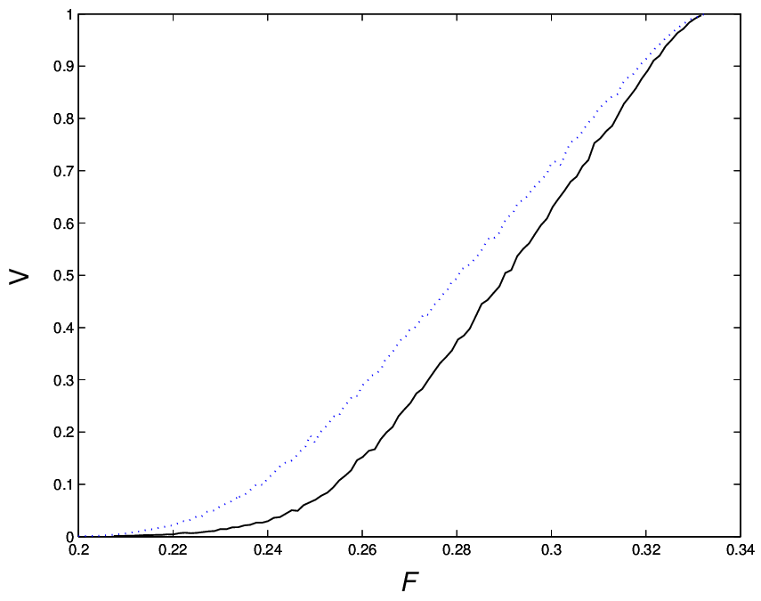
Refer to caption
Figure 7: Normalized volume VV of distilled Bell diagonal states compared to that of NPPT states for D=3D=3. The metric and the measuring algorithm are discussed in appendix G and uses Monte Carlo.

VI Conclusions and Prospects

We have shown that the study of entanglement distillation protocols based on the recursion method bennett1 is greatly benefited from the application of basic number theory concepts when the set 𝐙Dn\mathbf{Z}_{D}^{n} associated to qudits of arbitrary dimensions DD is a module, and not a vector space. In particular, we have found that a partition of 𝐙Dn\mathbf{Z}_{D}^{n} into divisor classes is very useful to characterize the invariant properties of mixed Bell diagonal states under unitary groups that implement local permutations. This permutations, in turn, are used in very general distillation protocols based on the recursion method.

We have proposed and study a variety of distillation protocols that fall into two classes depending on whether we use twirling operations or not at intermediate steps of the protocols. When the twirling operations are absent, our distillation protocols amount to extensions of the quantum privacy amplification protocols qpa valid for arbitrary qudit dimensions DD. This is very interesting and relevant for quantum commmunications with arbitrary large alphabets since they remain secure and operative even in the presence of quantum noisy channels.

These properties obtained from number theory are not only useful in the analytical understanding of the protocols, but also facilitate a lot the construction of numerical methods for their study using Monte Carlo. In particular, we have characterized how the distillation protocols based on the recursion method and local permutations are qualitatively and quantitatively optimal when the dimension of the qudit states DD is a prime number. We leave open the problem of how to construct better distillation protocols when DD is not a prime number and in this regard, the use of the heterotropic states introduced here is a promising tool.

Acknowledgements We acknowledge financial support from a PFI fellowship of the EJ-GV (H.B.) and DGS grant under contract BFM 2003-05316-C02-01 (M.A.MD.).

Appendix A Properties of the Module 𝐙Dn\mathbf{Z}_{D}^{n}

In this appendix we show how many ideas from genuine vector spaces can be adapted to the module 𝐙Dn\mathbf{Z}_{D}^{n}. First of all, we say that an element of s∈𝐙Ds\in\mathbf{Z}_{D} is invertible if there exists s′∈𝐙Ds^{\prime}\in\mathbf{Z}_{D} such that s​s′=1ss^{\prime}=1. If x∈𝐍x\in\mathbf{N} is a representant of ss, this is equivalent to gcd⁡(x,D)=1\gcd(x,D)=1. When DD is not prime, non invertible elements other than zero exist (they are multiples of proper divisors of D) and we need to introduce a work around in the gaussian elimination method, as we shall explain now.

Suppose we are given an element of 𝐙D2\mathbf{Z}_{D}^{2}, say (x,y)(x,y), and we are asked to get x=0x=0 using two elementary transformations:

(x,y)​⟶𝒪1​(x,x+y),(x,y)​⟶𝒪2​(x+y,y),(x,y)\overset{\mathcal{O}_{1}}{\longrightarrow}(x,x+y),\qquad(x,y)\overset{\mathcal{O}_{2}}{\longrightarrow}(x+y,y), (85)

The algorithm turns out to be quite simple. Consider for a moment the arbitrary ordering in 𝐙D\mathbf{Z}_{D} 0<1<⋯<D−10<1<\cdots<{D-1}. At each step, if x≤yx\leq y use 𝒪1\mathcal{O}_{1} to get 0≤y<x0\leq y<x, proceed inversely on the contrary. Clearly, x=0x=0 or y=0y=0 is reached in a finite number of steps. If y=0y=0, just apply 𝒪1\mathcal{O}_{1} once and 𝒪2\mathcal{O}_{2} D−1D-1 times.

We shall use gaussian elimination, with the aid of the above trick, to convert any matrix MM of size p×qp\times q into a very simple one. Suppose p≤qp\leq q; the converse case is similar. Summing one row to another amounts to take the product (from the left) with a p×pp\times p invertible matrix. The same is true for columns (from the right, q×qq\times q). Using this elementary operations we can obtain:

C=A​M​B,C=[D0],C=AMB,\qquad C=\begin{bmatrix}D&0\end{bmatrix}, (86)

where AA and BB are invertible and DD is a diagonal matrix.

With this tool at hand, we are ready to start with our analysis. We adopt the usual definition of linear independence for a finite subset of 𝐙Dn\mathbf{Z}_{D}^{n}, but the following is more surprising:

Definition A.1

Consider any M∈𝐌p×q​(𝐙D)M\in\mathbf{M}_{p\times q}(\mathbf{Z}_{D}) and let SrS_{r} be the set of all r×rr\times r minors of MM, r∈R:={1,…,min⁡(p,q)}r\in R:=\{1,\dots,\min(p,q)\}. The rank of M is defined as

rank⁡(M):=max⁡{0}∪{r∈R:gcd⁡(Sr)=1}.\mathrm{rank}(M):=\max\;\{0\}\cup\{\,r\in R:\gcd(S_{r})=1\,\}. (87)

The rank of a matrix does not vary when we apply the elementary operations discussed above (see (14) and take into account that d|xd|x and d|yd|y iff d|xd|x and d|x+yd|x+y). As expected, a square matrix is invertible iff its rank is maximal. The following statement clarifies this strange definition:

Proposition A.2

The rows of a matrix M∈𝐌p×n​(𝐙D)M\in\mathbf{M}_{p\times n}(\mathbf{Z}_{D}) form a l.i. set iff rank⁡(M)=p\mathrm{rank}(M)=p.

Proof. Recall decomposition (86) for MM (we will use directly the notation there) and consider any 𝐯∈𝐙Dp\boldsymbol{\mathrm{v}}\in\mathbf{Z}_{D}^{p}:

𝐯t​M=0⇔𝐯t​A−1​C​B−1=0⇔𝐯′t​C=0,\boldsymbol{\mathrm{v}}^{t}M=0\iff\boldsymbol{\mathrm{v}}^{t}A^{-1}CB^{-1}=0\iff{\boldsymbol{\mathrm{v}}^{\prime}}^{t}C=0,

where 𝐯=At​𝐯′\boldsymbol{\mathrm{v}}=A^{t}\boldsymbol{\mathrm{v}}^{\prime}. This shows that the rows of MM form a l.i. set iff the rows of CC do. On the other hand, rank⁡(C)=rank⁡(M)\mathrm{rank}(C)=\mathrm{rank}(M), and for the matrix CC the statement is trivial. □\square

Given a set S={𝐯1,…,𝐯k}⊂𝐙DnS=\{\boldsymbol{\mathrm{v}}_{1},\dots,\boldsymbol{\mathrm{v}}_{k}\}\subset\mathbf{Z}_{D}^{n}, we will denote by Lin​S\mathrm{Lin}\,S the subset of 𝐙Dn\mathbf{Z}_{D}^{n} spanned by the elements of SS, that is, the set of linear combinations of the vectors in SS. Clearly, if SS is l.i. ♯​Lin​S=Dk\sharp\mathrm{Lin}\,S=D^{k}, and so k≤nk\leq n. Not surprisingly, any l.i. set which spans 𝐙D\mathbf{Z}_{D} will be called a base of 𝐙Dn\mathbf{Z}_{D}^{n}. The usual definition of subspace does not work, however, and we introduce in its place the following:

Definition A.3

A set V⊂𝐙DnV\subset\mathbf{Z}_{D}^{n} is said to be a subspace of 𝐙Dn\mathbf{Z}_{D}^{n} if V={0}V=\{0\} or if there exists a set S={𝐯1,…,𝐯k}⊂𝐙DnS=\{\boldsymbol{\mathrm{v}}_{1},\dots,\boldsymbol{\mathrm{v}}_{k}\}\subset\mathbf{Z}_{D}^{n} such that it is l.i. and Lin​S=V\mathrm{Lin}\,S=V. Such a set is called a base of VV, and its cardinality is the dimension of VV (dimV)(\dim V).

Dimension is well defined since ♯​V=D♯​S\sharp V=D^{\sharp S} forbids the possibility of two bases of different cardinality.

Proposition A.4

Given a set S={𝐯1,…,𝐯k}⊂𝐙DnS=\{\boldsymbol{\mathrm{v}}_{1},\dots,\boldsymbol{\mathrm{v}}_{k}\}\subset\mathbf{Z}_{D}^{n} which is linearly independent, there exists a set S′={𝐯k+1,…,𝐯n}S^{\prime}=\{\boldsymbol{\mathrm{v}}_{k+1},\dots,\boldsymbol{\mathrm{v}}_{n}\} such that S∪S′S\cup S^{\prime} is a base of 𝐙D\mathbf{Z}_{D}.

Proof. Let MM be a k×nk\times n matrix such that its rows are the elements of SS. We recall (86) but rewrite it in terms of n×nn\times n square matrices:

[D000]=[A001]​[M0]​B\begin{bmatrix}D&0\\ 0&0\end{bmatrix}=\begin{bmatrix}A&0\\ 0&1\end{bmatrix}\begin{bmatrix}M\\ 0\end{bmatrix}B (88)

Now consider the following:

[MM′]=[A−1001]​[D001]​B−1\begin{bmatrix}M\\ M^{\prime}\end{bmatrix}=\begin{bmatrix}A^{-1}&0\\ 0&1\end{bmatrix}\begin{bmatrix}D&0\\ 0&1\end{bmatrix}B^{-1} (89)

It is enough to construct S′S^{\prime} with the rows of M′M^{\prime}. □\square

Corolary A.5

Given a subspace VV of dimension dd and a set S={𝐯1,…,𝐯k}⊂VS=\{\boldsymbol{\mathrm{v}}_{1},\dots,\boldsymbol{\mathrm{v}}_{k}\}\subset V which is linearly independent, there exists a set S′={𝐯k+1,…,𝐯d}S^{\prime}=\{\boldsymbol{\mathrm{v}}_{k+1},\dots,\boldsymbol{\mathrm{v}}_{d}\} such that S∪S′S\cup S^{\prime} is a base of VV.

Proof. Select any base of VV and consider the components of vectors respect to that base as elements of 𝐙Dd\mathbf{Z}_{D}^{d}. □\square

We adopt the usual definition and notations for the scalar product and orthogonality.

Proposition A.6

The subset of 𝐙Dn\mathbf{Z}_{D}^{n} orthogonal to a subspace VV (that is, V⊥V^{\bot}) is a subspace. Moreover, dimV+dimV⊥=n\dim V+\dim V^{\bot}=n.

Proof. Let d=dimVd=\dim V and let MM be a d×nd\times n matrix such that its rows form a base of VV. We use decomposition (86) (again). For any 𝐯∈𝐙Dn\boldsymbol{\mathrm{v}}\in\mathbf{Z}_{D}^{n}

M​𝐯=0⇔A−1​C​B−1​𝐯=0⇔C⁡(𝐯′)=0,M\boldsymbol{\mathrm{v}}=0\iff A^{-1}CB^{-1}\boldsymbol{\mathrm{v}}=0\iff C(\boldsymbol{\mathrm{v}}^{\prime})=0, (90)

with 𝐯=B​𝐯′\boldsymbol{\mathrm{v}}=B\boldsymbol{\mathrm{v}}^{\prime}. The set of the 𝐯′\boldsymbol{\mathrm{v}}^{\prime}-s verifying the equation is clearly a subspace of the expected dimension. □\square

Appendix B Cardinality of Cd​(D,n)C_{d}(D,n): generalized Euler’s totient function

This appendix is devoted to the proof of lemma II.2. We start with part 2, which can be rewritten as:

♯​C1​(D,n)=♯​Cd​(d​D,n)∀D≥2,n≥1,d≥1\sharp C_{1}(D,n)=\sharp C_{d}(dD,n)\qquad\forall\>D\geq 2,n\geq 1,d\geq 1 (91)

This is equivalent to the existence of a one to one mapping from C1​(D,n)C_{1}(D,n) onto Cd​(d​D,n)C_{d}(dD,n). Consider the mapping:

μ:𝐙n\displaystyle\mu:\mathbf{Z}^{n} ⟶𝐙n\displaystyle\longrightarrow\mathbf{Z}^{n} (92)
𝐯\displaystyle\boldsymbol{\mathrm{v}} ⟶d​𝐯\displaystyle\longrightarrow d\boldsymbol{\mathrm{v}} (93)

μ\mu induces a mapping μ¯:𝐙Dn→𝐙d​Dn\overline{\mu}:\mathbf{Z}_{D}^{n}\rightarrow\mathbf{Z}_{dD}^{n}, which is well defined and one-to-one because x=y(modD)⇔d​x=d​y(modd​D)x=y\pmod{D}\Leftrightarrow dx=dy\pmod{dD}. From 14 we learn that ∀𝐯∈𝐙n\forall\>\boldsymbol{\mathrm{v}}\in\mathbf{Z}^{n}

d|gcd⁡(μ¯​(𝐯¯)),d|\gcd(\overline{\mu}(\overline{\boldsymbol{\mathrm{v}}})),

where 𝐯¯\overline{\boldsymbol{\mathrm{v}}} is the result of mapping 𝐯\boldsymbol{\mathrm{v}} in 𝐙Dn\mathbf{Z}_{D}^{n}. Since for any x∈𝐙x\in\mathbf{Z} and d′∈div⁡(D)d^{\prime}\in\mathrm{div}(D) we have d′|x⇔d′​d|d​xd^{\prime}|x\Leftrightarrow d^{\prime}d|dx, it follows that

d​gcd⁡(𝐯¯)=gcd⁡(μ¯​(𝐯¯)),d\gcd(\overline{\boldsymbol{\mathrm{v}}})=\gcd(\overline{\mu}(\overline{\boldsymbol{\mathrm{v}}})), (94)

which implies that C1​(D,n)C_{1}(D,n) is mapped into Cd​(d​D,n)C_{d}(dD,n). Since for any element of Cd​(d​D,n)C_{d}(dD,n) there exists a suitable 𝐯\boldsymbol{\mathrm{v}}, the mapping is onto.

Now proving part 1 of the lemma is easy. Start with

ϕn​(D)=Dn−∑d∈div⁡(D)−{1}♯​Cd​(D,n)=Dn−∑d∈div⁡(D)−{1}ϕn​(Dd).\begin{split}\phi_{n}(D)&=D^{n}-\sum_{d\in\mathrm{div}(D)-\{1\}}\sharp C_{d}(D,n)\\ &=D^{n}-\sum_{d\in\mathrm{div}(D)-\{1\}}\phi_{n}(\frac{D}{d}).\end{split} (95)

Changing the index, we get a beautiful recursive relation:

ϕn​(D)=Dn−∑d∈div⁡(D)−{D}ϕn​(d).\phi_{n}(D)=D^{n}-\sum_{d\in\mathrm{div}(D)-\{D\}}\phi_{n}(d). (96)

With some algebra on this expression it is possible to show that ϕn​(D)\phi_{n}(D) is a multiplicative function: A function f:𝐍→𝐍f:\mathbf{N}\rightarrow\mathbf{N} is said to be multiplicative if f⁡(n​m)=f⁡(n)​f​(m)f(nm)=f(n)f(m) ∀n,m∈𝐍\forall\>n,m\in\mathbf{N} such that gcd⁡(m,n)=1\gcd(m,n)=1. Thus, we only have to solve the recursion for D=pqD=p^{q}, pp prime, but this poses no difficulty:

ϕn​(pq)=pn​q−p(n−1)​q,\phi_{n}(p^{q})=p^{nq}-p^{(n-1)q}, (97)

from which (17) follows.

Part 3 of the lemma is nothing but the recursion relation just constructed.

Appendix C Generators of 𝒫S\mathcal{P}_{\scriptscriptstyle{\mathrm{S}}}

In order to study 𝒫S\mathcal{P}_{\scriptscriptstyle{\mathrm{S}}} it is preferable to consider its elements as permutations over 𝐙Dn×𝐙Dn\mathbf{Z}_{D}^{n}\times\mathbf{Z}_{D}^{n}, and so we change the notation

𝐱\displaystyle\boldsymbol{\mathrm{x}} ⟶π⁡(𝐱),\displaystyle\longrightarrow\pi(\boldsymbol{\mathrm{x}}),\quad 𝐱∈𝐙D2​n\displaystyle\boldsymbol{\mathrm{x}}\in\mathbf{Z}_{D}^{2n} (98)
for
(𝐢,𝐣)\displaystyle(\boldsymbol{\mathrm{i}},\boldsymbol{\mathrm{j}}) ⟶(μ⁡(𝐢,𝐣),ν⁡(𝐢,𝐣)),\displaystyle\longrightarrow(\mu(\boldsymbol{\mathrm{i}},\boldsymbol{\mathrm{j}}),\nu(\boldsymbol{\mathrm{i}},\boldsymbol{\mathrm{j}})),\quad 𝐢,𝐣∈𝐙Dn.\displaystyle\boldsymbol{\mathrm{i}},\boldsymbol{\mathrm{j}}\in\mathbf{Z}_{D}^{n}. (99)

where the correspondence is the same as in (11).

Lemma C.1

𝒫S\mathcal{P}_{\scriptscriptstyle{\mathrm{S}}} is generated by its following elements:

π+1, with μ⁡(𝐢,𝐣)\displaystyle\pi_{+}^{1},\quad\text{ with }\quad\mu(\boldsymbol{\mathrm{i}},\boldsymbol{\mathrm{j}}) =𝐢,\displaystyle=\boldsymbol{\mathrm{i}},
ν⁡(𝐢,𝐣)\displaystyle\nu(\boldsymbol{\mathrm{i}},\boldsymbol{\mathrm{j}}) =(i1+j1,j2,…,jn);\displaystyle=(i_{1}+j_{1},j_{2},\dots,j_{n});
πxch1, with μ⁡(𝐢,𝐣)\displaystyle\pi_{\mathrm{xch}}^{1},\quad\text{ with }\quad\mu(\boldsymbol{\mathrm{i}},\boldsymbol{\mathrm{j}}) =(j1,i2,…,in),\displaystyle=(j_{1},i_{2},\dots,i_{n}),
ν⁡(𝐢,𝐣)\displaystyle\nu(\boldsymbol{\mathrm{i}},\boldsymbol{\mathrm{j}}) =(−i1,j2,…,jn);\displaystyle=(-i_{1},j_{2},\dots,j_{n});
π+12, with μ⁡(𝐢,𝐣)\displaystyle\pi_{+}^{12},\quad\text{ with }\quad\mu(\boldsymbol{\mathrm{i}},\boldsymbol{\mathrm{j}}) =(i1+i2,i2,…,in),\displaystyle=(i_{1}+i_{2},i_{2},\dots,i_{n}),
ν⁡(𝐢,𝐣)\displaystyle\nu(\boldsymbol{\mathrm{i}},\boldsymbol{\mathrm{j}}) =(j1,j2−j1,…,jn);\displaystyle=(j_{1},j_{2}-j_{1},\dots,j_{n});
πswapl​m, with μ⁡(𝐢,𝐣)\displaystyle\pi_{\mathrm{swap}}^{lm},\quad\text{ with }\quad\mu(\boldsymbol{\mathrm{i}},\boldsymbol{\mathrm{j}}) =(…,il−1,im,il+1,…CLOSE,\displaystyle=(\dots,i_{l-1},i_{m},i_{l+1},\dots,
OPENim−1,il,im+1,…),\displaystyle i_{m-1},i_{l},i_{m+1},\dots),
ν⁡(𝐢,𝐣)\displaystyle\nu(\boldsymbol{\mathrm{i}},\boldsymbol{\mathrm{j}}) =(…,jl−1,jm,jl+1,…CLOSE,\displaystyle=(\dots,j_{l-1},j_{m},j_{l+1},\dots,
OPENjm−1,jl,jm+1,…),l,m=1,…,n.\displaystyle j_{m-1},j_{l},j_{m+1},\dots),\ \ l,m=1,\dots,n.

Proof. In order to proof this, first let us define

π+i\displaystyle\pi_{+}^{i} :=πswap1​i∘π+1∘πswap1​i,\displaystyle:=\pi_{\mathrm{swap}}^{1i}\circ\pi_{+}^{1}\circ\pi_{\mathrm{swap}}^{1i}, (100)
πxchi\displaystyle\pi_{\mathrm{xch}}^{i} :=πswap1​i∘πxch1∘πswap1​i,\displaystyle:=\pi_{\mathrm{swap}}^{1i}\circ\pi_{\mathrm{xch}}^{1}\circ\pi_{\mathrm{swap}}^{1i}, (101)
π+i​j\displaystyle\pi_{+}^{ij} :=πswap1​i∘πswap2​j∘π+12∘πswap1​i∘πswap2​j,\displaystyle:=\pi_{\mathrm{swap}}^{1i}\circ\pi_{\mathrm{swap}}^{2j}\circ\pi_{+}^{12}\circ\pi_{\mathrm{swap}}^{1i}\circ\pi_{\mathrm{swap}}^{2j}, (102)

with i,j=1,…,ni,j=1,\dots,n. Consider any p∈𝒫Sp\in\mathcal{P}_{\scriptscriptstyle{\mathrm{S}}}; our goal is to act from the left and from the right with these permutations till we get the identity, which is equivalent to the statement of the lemma. We shall use the matrix representation of the permutations, and the process is a suitable gaussian elimination similar to the one used in appendix A. The difference is that now we cannot perform freely any sum of lines or columns, but only those which have associated a permutation in the above set.

To work around this problem, in place of (85) we consider

(x,y)​⟶𝒪1​(x,x+y),(x,y)​⟶𝒪3​(e)​(e​y,x),e=±1(x,y)\overset{\mathcal{O}_{1}}{\longrightarrow}(x,x+y),\qquad(x,y)\overset{\mathcal{O}_{3}(e)}{\longrightarrow}(ey,x),\quad e=\pm 1 (103)

Since 𝒪2\mathcal{O}_{2} can be constructed suitably combining 𝒪1\mathcal{O}_{1} and 𝒪3​(−1)\mathcal{O}_{3}(-1), only the case e=1e=1 is really different, but adapting the algorithm is straightforward. The point is that π+i\pi_{+}^{i} and π+i​j\pi_{+}^{ij} can be attached to 𝒪1\mathcal{O}_{1}, πxchi\pi_{\mathrm{xch}}^{i} to 𝒪3​(−1)\mathcal{O}_{3}(-1) and πswapi​j\pi_{\mathrm{swap}}^{ij} to 𝒪3​(1)\mathcal{O}_{3}(1), with care in the case of π+i​j\pi_{+}^{ij} and πswapi​j\pi_{\mathrm{swap}}^{ij} for their additional effects.

To perform the elimination in an element of 𝒫S\mathcal{P}_{\scriptscriptstyle{\mathrm{S}}} with associated matrix MM, start working over the first column (permutations act thereby from the left). Using p+ip_{+}^{i} and pe​xip_{ex}^{i} make zero the elements Mn+1,1M_{n+1,1} to M2​n,1M_{2n,1}, and then use p+1​ip_{+}^{1i} and ps​w​a​p1​ip_{swap}^{1i} till just M11M_{11} is nonzero in the first column. The process must be repeated for the first row (this time permutations act from the right). Now let us deal with the second column, first making zero the elements Mn+2,2M_{n+2,2} to M2​n,2M_{2n,2}, afterwards the elements M3,2M_{3,2} to Mn,2M_{n,2}. Do the same for the second row. The process must be carried out for the first nn rows and columns, till we get something of the form

[DT1T2M],\begin{bmatrix}D&T_{1}\\ T_{2}&M\end{bmatrix}, (104)

with DD diagonal, T1T_{1} lower triangular and T2T_{2} upper triangular. But in fact applying the condition (28) forces T1=T2=0T_{1}=T_{2}=0 and M=D−1M=D^{-1}. Now we note that

[D00D−1]=[10−D1]​[10D−11]​[1101].\begin{bmatrix}D&0\\ 0&D^{-1}\end{bmatrix}=\begin{bmatrix}1&0\\ -D&1\end{bmatrix}\begin{bmatrix}1&0\\ D-1&1\end{bmatrix}\begin{bmatrix}1&1\\ 0&1\end{bmatrix}. (105)

Since the matrices in the right side are trivially constructed with the given set of generators, this ends the proof. □\square

Appendix D Proof of theorem III.1

(This proof uses the notation and results of appendix C)

(1) Since 𝒫T\mathcal{P}_{\scriptscriptstyle{\mathrm{T}}} is invariant in the product group trivially, we prove both sides of the inclusion, starting with 𝒫loc⊂𝒫T⋉𝒫S\mathcal{P}_{\scriptscriptstyle{\mathrm{loc}}}\subset\mathcal{P}_{\scriptscriptstyle{\mathrm{T}}}\ltimes\mathcal{P}_{\scriptscriptstyle{\mathrm{S}}}.

Later we define local unitary operators implementing 𝒫T\mathcal{P}_{\scriptscriptstyle{\mathrm{T}}} (see (112)), and so we just bother about those U∈𝒰B​loc​(D,n)U\in\mathcal{U}_{\scriptscriptstyle{\mathrm{B\,loc}}}(D,n) that leave |0 0⟩​ℬ​ ​⟨0 0||0\;0\rangle\!\text{\hskip 0.86108pt}\text{\raisebox{-2.15277pt}{${\scriptscriptstyle{\mathcal{B}}}$}}\!\text{\hskip 1.07639pt}\langle 0\;0| invariant. Moreover, as the global phase is unimportant, we select for the analysis those operators for which U​|0 0⟩​ℬ=|0 0⟩​ℬU|0\;0\rangle\!\text{\hskip 0.86108pt}\text{\raisebox{-2.15277pt}{${\scriptscriptstyle{\mathcal{B}}}$}}=|0\;0\rangle\!\text{\hskip 0.86108pt}\text{\raisebox{-2.15277pt}{${\scriptscriptstyle{\mathcal{B}}}$}}. But UU is local, and then these constraints are equivalent to U=UA⊗UA∗U=U_{\rm A}\otimes U_{\rm A}^{\ast} (conjugation respect to the computational basis). We can thus write:

U⁡|𝐢​𝐣⟩=𝒮𝐤𝐥​A𝐤𝐢​A𝐥𝐣∗​|𝐤​𝐥⟩,𝒮𝐤​A𝐢𝐤​A𝐣𝐤∗=δ⁡(𝐢−𝐣)U|\boldsymbol{\mathrm{i}}\;\boldsymbol{\mathrm{j}}\rangle={{\underset{\text{\raisebox{-0.60275pt}{$\boldsymbol{\mathrm{k}}\boldsymbol{\mathrm{l}}$}}}{\raisebox{-2.58334pt}{\text{\LARGE$\mathcal{S}$}}}}}A_{\boldsymbol{\mathrm{k}}\boldsymbol{\mathrm{i}}}A_{\boldsymbol{\mathrm{l}}\boldsymbol{\mathrm{j}}}^{*}\,|\boldsymbol{\mathrm{k}}\;\boldsymbol{\mathrm{l}}\rangle,\qquad{{\underset{\text{\raisebox{-0.60275pt}{$\boldsymbol{\mathrm{k}}$}}}{\raisebox{-2.58334pt}{\text{\LARGE$\mathcal{S}$}}}}}A_{\boldsymbol{\mathrm{i}}\boldsymbol{\mathrm{k}}}A^{\ast}_{\boldsymbol{\mathrm{j}}\boldsymbol{\mathrm{k}}}=\delta(\boldsymbol{\mathrm{i}}-\boldsymbol{\mathrm{j}}) (106)

with AA a unitary matrix on a single party (Alice or Bob). Using (5), we get

U⁡|𝐢​𝐣⟩​ℬ=𝒮𝐤𝐥𝐦𝐧​φ​(𝐤⋅𝐢−𝐦⋅𝐥)​A𝐥𝐤​A𝐥−𝐧,𝐤−𝐣∗​|𝐦​𝐧⟩​ℬ.U|\boldsymbol{\mathrm{i}}\;\boldsymbol{\mathrm{j}}\rangle\!\text{\hskip 0.86108pt}\text{\raisebox{-2.15277pt}{${\scriptscriptstyle{\mathcal{B}}}$}}={{\underset{\text{\raisebox{-0.60275pt}{$\boldsymbol{\mathrm{k}}\boldsymbol{\mathrm{l}}\boldsymbol{\mathrm{m}}\boldsymbol{\mathrm{n}}$}}}{\raisebox{-2.58334pt}{\text{\LARGE$\mathcal{S}$}}}}}\varphi(\boldsymbol{\mathrm{k}}\cdot\boldsymbol{\mathrm{i}}-\boldsymbol{\mathrm{m}}\cdot\boldsymbol{\mathrm{l}})A_{\boldsymbol{\mathrm{l}}\boldsymbol{\mathrm{k}}}A_{\boldsymbol{\mathrm{l}}-\boldsymbol{\mathrm{n}},\boldsymbol{\mathrm{k}}-\boldsymbol{\mathrm{j}}}^{\ast}\,|\boldsymbol{\mathrm{m}}\;\boldsymbol{\mathrm{n}}\rangle\!\text{\hskip 0.86108pt}\text{\raisebox{-2.15277pt}{${\scriptscriptstyle{\mathcal{B}}}$}}. (107)

On the other hand, the action of UU involves a permutation over Bell states:

U⁡|𝐢​𝐣⟩​ℬ=ϕ⁡(𝐢,𝐣)​|μ⁡(𝐢,𝐣)​ν​(𝐢,𝐣)⟩​ℬ.U|\boldsymbol{\mathrm{i}}\;\boldsymbol{\mathrm{j}}\rangle\!\text{\hskip 0.86108pt}\text{\raisebox{-2.15277pt}{${\scriptscriptstyle{\mathcal{B}}}$}}=\phi(\boldsymbol{\mathrm{i}},\boldsymbol{\mathrm{j}})\,|\mu(\boldsymbol{\mathrm{i}},\boldsymbol{\mathrm{j}})\;\nu(\boldsymbol{\mathrm{i}},\boldsymbol{\mathrm{j}})\rangle\!\text{\hskip 0.86108pt}\text{\raisebox{-2.15277pt}{${\scriptscriptstyle{\mathcal{B}}}$}}. (108)

Identifying both expressions (Bell states are orthogonal):

ϕ⁡(𝐢,𝐣)​δ​(𝐦−μ⁡(𝐢,𝐣))​δ​(𝐧−ν⁡(𝐢,𝐣))=𝒮𝐤𝐥​φ​(𝐤⋅𝐢−𝐥⋅𝐦)​A𝐥𝐤​A𝐥−𝐧,𝐤−𝐣∗.\phi(\boldsymbol{\mathrm{i}},\boldsymbol{\mathrm{j}})\,\delta(\boldsymbol{\mathrm{m}}-\mu(\boldsymbol{\mathrm{i}},\boldsymbol{\mathrm{j}}))\,\delta(\boldsymbol{\mathrm{n}}-\nu(\boldsymbol{\mathrm{i}},\boldsymbol{\mathrm{j}}))=\\ {{\underset{\text{\raisebox{-0.60275pt}{$\boldsymbol{\mathrm{k}}\boldsymbol{\mathrm{l}}$}}}{\raisebox{-2.58334pt}{\text{\LARGE$\mathcal{S}$}}}}}\varphi(\boldsymbol{\mathrm{k}}\cdot\boldsymbol{\mathrm{i}}-\boldsymbol{\mathrm{l}}\cdot\boldsymbol{\mathrm{m}})A_{\boldsymbol{\mathrm{l}}\boldsymbol{\mathrm{k}}}A_{\boldsymbol{\mathrm{l}}-\boldsymbol{\mathrm{n}},\boldsymbol{\mathrm{k}}-\boldsymbol{\mathrm{j}}}^{\ast}. (109)

Act on both sides of this equation with the Fourier operator 𝒮𝐦𝐧​φ​(𝐫⋅𝐦)​A𝐫−𝐧,𝐬−𝐣{\text{\Large$\mathcal{S}$}}_{\boldsymbol{\mathrm{m}}\boldsymbol{\mathrm{n}}}\,\varphi(\boldsymbol{\mathrm{r}}\cdot\boldsymbol{\mathrm{m}})A_{\boldsymbol{\mathrm{r}}-\boldsymbol{\mathrm{n}},\boldsymbol{\mathrm{s}}-\boldsymbol{\mathrm{j}}} to obtain:

A𝐫−ν⁡(𝐢,𝐣),𝐬−𝐣=φ⁡(𝐬⋅𝐢−𝐫⋅μ⁡(𝐢,𝐣))​ϕ​(𝐢,𝐣)∗​A𝐫,𝐬.A_{\boldsymbol{\mathrm{r}}-\nu(\boldsymbol{\mathrm{i}},\boldsymbol{\mathrm{j}}),\boldsymbol{\mathrm{s}}-\boldsymbol{\mathrm{j}}}=\varphi(\boldsymbol{\mathrm{s}}\cdot\boldsymbol{\mathrm{i}}-\boldsymbol{\mathrm{r}}\cdot\mu(\boldsymbol{\mathrm{i}},\boldsymbol{\mathrm{j}}))\,\phi(\boldsymbol{\mathrm{i}},\boldsymbol{\mathrm{j}})^{\ast}A_{\boldsymbol{\mathrm{r}},\boldsymbol{\mathrm{s}}}. (110)

Choose any 𝐫,𝐬\boldsymbol{\mathrm{r}},\boldsymbol{\mathrm{s}} such that A𝐫𝐬≠0A_{\boldsymbol{\mathrm{r}}\boldsymbol{\mathrm{s}}}\neq 0, interpret this equation as a recurrence relation and consider the commutative diagram:

A𝐫𝐬⟶A𝐫−𝝅⁡(𝐢,𝐣),𝐬−𝐣↓↓A𝐫−𝝅⁡(𝐢′,𝐣′),𝐬−𝐣′⟶A𝐫−𝝅⁡(𝐢,𝐣)−𝝅⁡(𝐢′,𝐣′),𝐬−𝐣−𝐣′\begin{array}[]{ccc}A_{\boldsymbol{\mathrm{r}}\boldsymbol{\mathrm{s}}}&\longrightarrow&A_{\boldsymbol{\mathrm{r}}-\boldsymbol{\mathrm{\pi}}(\boldsymbol{\mathrm{i}},\boldsymbol{\mathrm{j}}),\boldsymbol{\mathrm{s}}-\boldsymbol{\mathrm{j}}}\\ \Big\downarrow&&\Big\downarrow\\ A_{\boldsymbol{\mathrm{r}}-\boldsymbol{\mathrm{\pi}}(\boldsymbol{\mathrm{i}}^{\prime},\boldsymbol{\mathrm{j}}^{\prime}),\boldsymbol{\mathrm{s}}-\boldsymbol{\mathrm{j}}^{\prime}}&\longrightarrow&A_{\boldsymbol{\mathrm{r}}-\boldsymbol{\mathrm{\pi}}(\boldsymbol{\mathrm{i}},\boldsymbol{\mathrm{j}})-\boldsymbol{\mathrm{\pi}}(\boldsymbol{\mathrm{i}}^{\prime},\boldsymbol{\mathrm{j}}^{\prime}),\boldsymbol{\mathrm{s}}-\boldsymbol{\mathrm{j}}-\boldsymbol{\mathrm{j}}^{\prime}}\end{array}

Switching again to the 𝐙D2​n\mathbf{Z}_{D}^{2n} notation, the commutation condition is

𝐱t​Ω​𝐱′=π​(𝐱)t​Ω​π​(𝐱′)\boldsymbol{\mathrm{x}}^{t}\,\Omega\,\boldsymbol{\mathrm{x}}^{\prime}=\pi(\boldsymbol{\mathrm{x}})^{t}\,\Omega\,\pi(\boldsymbol{\mathrm{x}}^{\prime}) (111)

for any 𝐱,𝐱′∈𝐙D2​n\boldsymbol{\mathrm{x}},\boldsymbol{\mathrm{x}}^{\prime}\in\mathbf{Z}_{D}^{2n}. Thus, π∈𝒫S\pi\in\mathcal{P}_{\scriptscriptstyle{\mathrm{S}}}.

We now show that 𝒫T⋉𝒫S⊂𝒫loc\mathcal{P}_{\scriptscriptstyle{\mathrm{T}}}\ltimes\mathcal{P}_{\scriptscriptstyle{\mathrm{S}}}\subset\mathcal{P}_{\scriptscriptstyle{\mathrm{loc}}}. Thanks to lemma C.1, it is enough to construct a few permutations by means of unitary local operators. We start with translations. Choosing

UA​|𝐢⟩=φ⁡(𝐢⋅𝐚)​|𝐢⟩,\displaystyle U_{\rm A}\,|\boldsymbol{\mathrm{i}}\rangle=\varphi(\boldsymbol{\mathrm{i}}\cdot\boldsymbol{\mathrm{a}})\,|\boldsymbol{\mathrm{i}}\rangle, UB​|𝐢⟩=|𝐢−𝐛⟩,\displaystyle\qquad U_{\rm B}\,|\boldsymbol{\mathrm{i}}\rangle=|\boldsymbol{\mathrm{i}}-\boldsymbol{\mathrm{b}}\rangle, (112)
with 𝐚,𝐛∈𝐙Dn\boldsymbol{\mathrm{a}},\boldsymbol{\mathrm{b}}\in\mathbf{Z}_{D}^{n}, the effect is
μ⁡(𝐢,𝐣)=𝐢+𝐚,\displaystyle\mu(\boldsymbol{\mathrm{i}},\boldsymbol{\mathrm{j}})=\boldsymbol{\mathrm{i}}+\boldsymbol{\mathrm{a}}, ν⁡(𝐢,𝐣)=𝐣+𝐛.\displaystyle\qquad\nu(\boldsymbol{\mathrm{i}},\boldsymbol{\mathrm{j}})=\boldsymbol{\mathrm{j}}+\boldsymbol{\mathrm{b}}.
This is not the only subgroup easily generated, we have also that
UA​|𝐢⟩=|S​𝐢⟩,\displaystyle U_{\rm A}\,|\boldsymbol{\mathrm{i}}\rangle=|S\boldsymbol{\mathrm{i}}\rangle, UB​|𝐢⟩=|S​𝐢⟩,\displaystyle\qquad U_{\rm B}\,|\boldsymbol{\mathrm{i}}\rangle=|S\boldsymbol{\mathrm{i}}\rangle, (113)
with S∈𝐙Dn×𝐙DnS\in\mathbf{Z}_{D}^{n}\times\mathbf{Z}_{D}^{n} and invertible give
μ⁡(𝐢,𝐣)=(St)−1​𝐢,\displaystyle\mu(\boldsymbol{\mathrm{i}},\boldsymbol{\mathrm{j}})=(S^{t})^{-1}\boldsymbol{\mathrm{i}}, ν⁡(𝐢,𝐣)=S​𝐣.\displaystyle\qquad\nu(\boldsymbol{\mathrm{i}},\boldsymbol{\mathrm{j}})=S\boldsymbol{\mathrm{j}}.

Both of these results can be checked with a few manipulations in (II.1). Since πswapl​m\pi_{\mathrm{swap}}^{lm} is physically trivial and π+l​m\pi_{+}^{lm} is contained in the last construction, the only permutations we have not still covered are π+1\pi_{+}^{1} and πxch1\pi_{\mathrm{xch}}^{1}, but as these involve only the first pair of qudits we can fix n=1n=1 in (110) and try the ansatz Al​k=φ⁡(η⁡(i,j))A_{lk}=\varphi(\eta(i,j)), with η⁡(i,j)∈𝐑/D\eta(i,j)\in\mathbf{R}/D. This results in:

η⁡(l−μ⁡(i,j),k−j)=η⁡(l,k)+k​i−l​ν​(i,j)−ϕ~​(i,j),\eta(l-\mu(i,j),k-j)=\eta(l,k)+ki-l\nu(i,j)-\tilde{\phi}(i,j), (114)

where φ⁡(ϕ~​(i,j)):=ϕ⁡(i,j)\varphi(\tilde{\phi}(i,j)):=\phi(i,j). Solutions to this equation require η\eta to be a second order polynomial, limiting the permutation to:

μ⁡(i,j)=a​j+b​ν​(i,j),ν⁡(i,j)=−a−1​(i+c​j),\mu(i,j)=aj+b\nu(i,j),\quad\nu(i,j)=-a^{-1}(i+cj), (115)

where a,b,c∈𝐙Da,b,c\in\mathbf{Z}_{D}, aa invertible. A compatible choice for η\eta is

η⁡(i,j)\displaystyle\eta(i,j) =a​i​j+b2​i2+c2​j2.\displaystyle=aij+\frac{b}{2}i^{2}+\frac{c}{2}j^{2}. (116)

The permutations we were searching for belong to the set of (115).

(2) In order to proof the second part of the theorem it is enough to analyze which are the realizations of the identity permutation. Going back to (110) and fixing μ⁡(𝐢,𝐣)=𝐢\mu(\boldsymbol{\mathrm{i}},\boldsymbol{\mathrm{j}})=\boldsymbol{\mathrm{i}} and ν⁡(𝐢,𝐣)=𝐣\nu(\boldsymbol{\mathrm{i}},\boldsymbol{\mathrm{j}})=\boldsymbol{\mathrm{j}} we find the equation

A𝐫−𝐣,𝐬−𝐣=φ⁡(𝐬⋅𝐢−𝐫⋅𝐢)​ϕ​(𝐢,𝐣)∗​A𝐫,𝐬.A_{\boldsymbol{\mathrm{r}}-\boldsymbol{\mathrm{j}},\boldsymbol{\mathrm{s}}-\boldsymbol{\mathrm{j}}}=\varphi(\boldsymbol{\mathrm{s}}\cdot\boldsymbol{\mathrm{i}}-\boldsymbol{\mathrm{r}}\cdot\boldsymbol{\mathrm{i}})\,\phi(\boldsymbol{\mathrm{i}},\boldsymbol{\mathrm{j}})^{\ast}A_{\boldsymbol{\mathrm{r}},\boldsymbol{\mathrm{s}}}. (117)

Modulo a global phase (30), the solutions are exactly of the form:

ϕ⁡(𝐢,𝐣)\displaystyle\phi(\boldsymbol{\mathrm{i}},\boldsymbol{\mathrm{j}}) =φ⁡(𝐚⋅𝐢+𝐛⋅𝐣)\displaystyle=\varphi(\boldsymbol{\mathrm{a}}\cdot\boldsymbol{\mathrm{i}}+\boldsymbol{\mathrm{b}}\cdot\boldsymbol{\mathrm{j}}) (118)
A𝐫𝐬\displaystyle A_{\boldsymbol{\mathrm{r}}\boldsymbol{\mathrm{s}}} =φ⁡(𝐛⋅𝐬)​δ​(𝐬−𝐫−𝐚)\displaystyle=\varphi(\boldsymbol{\mathrm{b}}\cdot\boldsymbol{\mathrm{s}})\delta(\boldsymbol{\mathrm{s}}-\boldsymbol{\mathrm{r}}-\boldsymbol{\mathrm{a}}) (119)

where 𝐚,𝐛∈𝐙Dn\boldsymbol{\mathrm{a}},\boldsymbol{\mathrm{b}}\in\mathbf{Z}_{D}^{n}. But this is U𝐱U_{\boldsymbol{\mathrm{x}}} in (30) with

𝐱=(b1,…,bn,−a1,…,−an).\boldsymbol{\mathrm{x}}=(b_{1},\dots,b_{n},-a_{1},\dots,-a_{n}). (120)

Appendix E Order of 𝒫S\mathcal{P}_{\scriptscriptstyle{\mathrm{S}}}

In this appendix we offer a proof of theorem III.2.

We first note that, except for a sign, 𝐮i\boldsymbol{\mathrm{u}}_{i} and 𝐯i\boldsymbol{\mathrm{v}}_{i} play interchangeable roles. Thus it is enough to consider a case with t=0t=0 (if t≥1t\geq 1, suitable exchanges between 𝐮\boldsymbol{\mathrm{u}}-s and 𝐯\boldsymbol{\mathrm{v}}-s and sign adjustments will be enough). We shall consider two cases separately, depending on wether r<nr<n. In both cases the target is to find out in how many ways a new vector can be included in the set. Such a vector must fulfill (III) and be linearly independent respect to the initial set.

Suppose r<nr<n. We would like to know how many vectors can take the role of 𝐮r+1\boldsymbol{\mathrm{u}}_{r+1}. Let S={𝐮1,…,𝐮r,𝐯1,…,𝐯s}S=\{\boldsymbol{\mathrm{u}}_{1},\dots,\boldsymbol{\mathrm{u}}_{r},\boldsymbol{\mathrm{v}}_{1},\dots,\boldsymbol{\mathrm{v}}_{s}\} and V=Lin​{Ω​𝐯:𝐯∈S}V=\mathrm{Lin}\,\{\,\,\Omega\,\boldsymbol{\mathrm{v}}:\boldsymbol{\mathrm{v}}\in S\,\}. From (III) we have 𝐮r+1∈V⊥\boldsymbol{\mathrm{u}}_{r+1}\in V^{\bot} (and no further conditions), so let S′={𝐮s+1,…,𝐮r,𝐰1,…,𝐰2​(n−r)}S^{\prime}=\{\boldsymbol{\mathrm{u}}_{s+1},\dots,\boldsymbol{\mathrm{u}}_{r},\boldsymbol{\mathrm{w}}_{1},\dots,\boldsymbol{\mathrm{w}}_{2(n-r)}\} be a base of V⊥V^{\bot}. We claim that S∪S′S\cup S^{\prime} is l.i., that is, the equation

∑i=1r−sai​𝐮s+j+∑i=12​(n−r)bi​𝐰i+∑i=1s(ci​𝐮i+di​𝐯i)=0\sum_{i=1}^{r-s}a_{i}\boldsymbol{\mathrm{u}}_{s+j}+\sum_{i=1}^{2(n-r)}b_{i}\boldsymbol{\mathrm{w}}_{i}+\sum_{i=1}^{s}(c_{i}\boldsymbol{\mathrm{u}}_{i}+d_{i}\boldsymbol{\mathrm{v}}_{i})=0

holds only if all the scalars are zero. This is so because taking the scalar product with Ω​𝐮k\,\Omega\,\boldsymbol{\mathrm{u}}_{k} (k≤sk\leq s) we get dk=0d_{k}=0; using Ω​𝐯k\,\Omega\,\boldsymbol{\mathrm{v}}_{k}, ck=0c_{k}=0. The rest of the scalars must be zero because S′S^{\prime} is l.i. Therefore there are Dr−s​ϕ2​(n−r)​(D)D^{r-s}\phi_{2(n-r)}(D) suitable vectors, since we can choose any combination of the form

𝐮r+1=∑i=1r−sai​𝐮s+j+∑i=12​(n−r)bi​𝐰i\boldsymbol{\mathrm{u}}_{r+1}=\sum_{i=1}^{r-s}a_{i}\boldsymbol{\mathrm{u}}_{s+j}+\sum_{i=1}^{2(n-r)}b_{i}\boldsymbol{\mathrm{w}}_{i}

for which gcd⁡({b1,…,b2​(n−r)})=1\gcd(\{b_{1},\dots,b_{2(n-r)}\})=1 (this is why the factor ϕ2​(n−r)​(D)\phi_{2(n-r)}(D) appears, see (16)).

Now suppose r=nr=n, s<ns<n. We pursue 𝐯s+1\boldsymbol{\mathrm{v}}_{s+1}. Let S={𝐮1,…,𝐮s,𝐮s+2,…,𝐮n,𝐯1,…,𝐯s}S=\{\boldsymbol{\mathrm{u}}_{1},\dots,\boldsymbol{\mathrm{u}}_{s},\boldsymbol{\mathrm{u}}_{s+2},\dots,\boldsymbol{\mathrm{u}}_{n},\boldsymbol{\mathrm{v}}_{1},\dots,\boldsymbol{\mathrm{v}}_{s}\} and V=Lin​{Ω​𝐯:𝐯∈S}V=\mathrm{Lin}\,\{\,\,\Omega\,\boldsymbol{\mathrm{v}}:\boldsymbol{\mathrm{v}}\in S\,\}. From (III) we have 𝐯s+1∈V⊥\boldsymbol{\mathrm{v}}_{s+1}\in V^{\bot} and 𝐮s+1t​Ω​𝐯s+1=1\boldsymbol{\mathrm{u}}_{s+1}^{t}\,\Omega\,\boldsymbol{\mathrm{v}}_{s+1}=1. Let S′={𝐮s+1,…,𝐮n,𝐰}S^{\prime}=\{\boldsymbol{\mathrm{u}}_{s+1},\dots,\boldsymbol{\mathrm{u}}_{n},\boldsymbol{\mathrm{w}}\} be a base of V⊥V^{\bot} and let s:=𝐮s+1t​Ω​𝐰s:=\boldsymbol{\mathrm{u}}_{s+1}^{t}\,\Omega\,\boldsymbol{\mathrm{w}}. We first show that ss is invertible. Let V′=Lin⁡{Ω​𝐮1,…,Ω​𝐮n,Ω​𝐯1,…,Ω​𝐯s}V^{\prime}=\mathrm{Lin}\,\{\,\Omega\,\boldsymbol{\mathrm{u}}_{1},\dots,\,\Omega\,\boldsymbol{\mathrm{u}}_{n},\,\Omega\,\boldsymbol{\mathrm{v}}_{1},\dots,\,\Omega\,\boldsymbol{\mathrm{v}}_{s}\}. If ss is non invertible, choose any k≠0k\neq 0 such that k​s=0ks=0. Then k​𝐮s+1t​Ω​𝐰=0k\boldsymbol{\mathrm{u}}_{s+1}^{t}\,\Omega\,\boldsymbol{\mathrm{w}}=0 implies k​𝐰∈V′⁣⊥=Lin⁡{𝐮s+1,…,𝐮n}k\boldsymbol{\mathrm{w}}\in V^{\prime\bot}=\mathrm{Lin}\,\{\boldsymbol{\mathrm{u}}_{s+1},\dots,\boldsymbol{\mathrm{u}}_{n}\}, but this is not possible because S′S^{\prime} is linearly independent. We now show that S∪{𝐮s+1,𝐰}S\cup\{\boldsymbol{\mathrm{u}}_{s+1},\boldsymbol{\mathrm{w}}\} is l.i. If it is not, then 𝐰∈Lin⁡(S∪{𝐮s+1})\boldsymbol{\mathrm{w}}\in\mathrm{Lin}\,(S\cup\{\boldsymbol{\mathrm{u}}_{s+1}\}), but this in turn implies 𝐮s+1t​Ω​𝐰=0\boldsymbol{\mathrm{u}}_{s+1}^{t}\,\Omega\,\boldsymbol{\mathrm{w}}=0, which again is false. Therefore, there are Dn−sD^{n-s} suitable vectors, since we can choose any of the following combinations:

𝐯s+1=s−1​𝐰+∑i=1n−sci​𝐮s+i.\boldsymbol{\mathrm{v}}_{s+1}=s^{-1}\boldsymbol{\mathrm{w}}+\sum_{i=1}^{n-s}c_{i}\boldsymbol{\mathrm{u}}_{s+i}.

With this, part 1 of the theorem is proved. For part 2, it only remains to count. There are ϕ2​n​(D)\phi_{2n}(D) possible values for 𝐮1\boldsymbol{\mathrm{u}}_{1}. If 𝐮1\boldsymbol{\mathrm{u}}_{1} is fixed, there are D​ϕ2​n​(D)D\phi_{2n}(D) possible elections for 𝐮2\boldsymbol{\mathrm{u}}_{2}. Continuing this way, one gets the desired result.

Appendix F Recursion Relations for Distillation Protocols

In this appendix we derive an expression for the final state of the remaining pairs of qudits when the procedure of section V has been successfully performed. We will use the same notation found there.

So let us define for 𝐱,𝐲∈𝐙D2​n\boldsymbol{\mathrm{x}},\boldsymbol{\mathrm{y}}\in\mathbf{Z}_{D}^{2n}

ρ𝐱𝐲(n)\displaystyle\rho^{\scriptscriptstyle(n)}_{\boldsymbol{\mathrm{x}}\boldsymbol{\mathrm{y}}} :=ℬ​ ​⟨𝐱|ρ(n)|𝐲⟩​ℬ,\displaystyle:=\text{\raisebox{-2.15277pt}{${\scriptscriptstyle{\mathcal{B}}}$}}\!\text{\hskip 1.07639pt}\langle\boldsymbol{\mathrm{x}}|\rho^{\scriptscriptstyle(n)}|\boldsymbol{\mathrm{y}}\rangle\!\text{\hskip 0.86108pt}\text{\raisebox{-2.15277pt}{${\scriptscriptstyle{\mathcal{B}}}$}}, (121)

from which p𝐱=ρ𝐱𝐱(n)p_{\boldsymbol{\mathrm{x}}}=\rho^{\scriptscriptstyle(n)}_{\boldsymbol{\mathrm{x}}\boldsymbol{\mathrm{x}}}. After the permutation with associated matrix MM and phase function ϕ\phi the state is

ρ(n)′:=∑𝐱,𝐲∈𝐙D2​nϕ⁡(𝐱)​ϕ∗​(𝐲)​ρ𝐱𝐲(n)​|M​𝐱⟩​ℬ​ ​⟨M​𝐲|.{\rho^{\scriptscriptstyle(n)}}^{\prime}:=\sum_{\boldsymbol{\mathrm{x}},\boldsymbol{\mathrm{y}}\in\mathbf{Z}_{D}^{2n}}\phi(\boldsymbol{\mathrm{x}})\phi^{\ast}(\boldsymbol{\mathrm{y}})\,\rho^{\scriptscriptstyle(n)}_{\boldsymbol{\mathrm{x}}\boldsymbol{\mathrm{y}}}\,|M\boldsymbol{\mathrm{x}}\rangle\!\text{\hskip 0.86108pt}\text{\raisebox{-2.15277pt}{${\scriptscriptstyle{\mathcal{B}}}$}}\!\text{\hskip 1.07639pt}\langle M\boldsymbol{\mathrm{y}}|. (122)

The measurement is performed in the computational basis (for the last n−mn-m pairs), and the rest of pairs are kept only if this measurement coincides for each of the measured pairs (if Alice measures |3⟩|3\rangle, so does Bob for the corresponding qudit). Going back to (5), this means that jj is zero for each of the pairs. Therefore after the measurement and taking the partial trace over the measured pairs the state of the first mm pairs is:

ρ(m)=1P​∑𝐤∈𝐙Dn−mℬ​ ​⟨𝐤​ 0|ρ(n)′|𝐤​ 0⟩​ℬ,\rho^{\scriptscriptstyle(m)}=\frac{1}{P}\sum_{\boldsymbol{\mathrm{k}}\in\mathbf{Z}_{D}^{n-m}}\text{\raisebox{-2.15277pt}{${\scriptscriptstyle{\mathcal{B}}}$}}\!\text{\hskip 1.07639pt}\langle\boldsymbol{\mathrm{k}}\;\boldsymbol{\mathrm{0}}|\,{\rho^{\scriptscriptstyle(n)}}^{\prime}\,|\boldsymbol{\mathrm{k}}\;\boldsymbol{\mathrm{0}}\rangle\!\text{\hskip 0.86108pt}\text{\raisebox{-2.15277pt}{${\scriptscriptstyle{\mathcal{B}}}$}}, (123)

where the Bell states must be understood to belong to the space of the last n−mn-m pairs and PP is the probability of having obtained the suitable measurement. Calculating it amounts to take the total trace:

P=∑𝐱∈𝐙D2​m∑𝐤∈𝐙Dn−m(ℬ​ ​⟨𝐱|⊗ℬ​ ​⟨𝐤​ 0|)​ρ(n)′​(|𝐱⟩​ℬ⊗|𝐤​ 0⟩​ℬ).P=\sum_{\boldsymbol{\mathrm{x}}\in\mathbf{Z}_{D}^{2m}}\sum_{\boldsymbol{\mathrm{k}}\in\mathbf{Z}_{D}^{n-m}}\left(\text{\raisebox{-2.15277pt}{${\scriptscriptstyle{\mathcal{B}}}$}}\!\text{\hskip 1.07639pt}\langle\boldsymbol{\mathrm{x}}|\otimes\text{\raisebox{-2.15277pt}{${\scriptscriptstyle{\mathcal{B}}}$}}\!\text{\hskip 1.07639pt}\langle\boldsymbol{\mathrm{k}}\;\boldsymbol{\mathrm{0}}|\right)\,{\rho^{\scriptscriptstyle(n)}}^{\prime}\,\left(|\boldsymbol{\mathrm{x}}\rangle\!\text{\hskip 0.86108pt}\text{\raisebox{-2.15277pt}{${\scriptscriptstyle{\mathcal{B}}}$}}\otimes|\boldsymbol{\mathrm{k}}\;\boldsymbol{\mathrm{0}}\rangle\!\text{\hskip 0.86108pt}\text{\raisebox{-2.15277pt}{${\scriptscriptstyle{\mathcal{B}}}$}}\right).

Inserting definition (122), we get (43).

The state of the system before the measurement can also be expressed

ρ(n)′=∑𝐱,𝐲∈𝐙D2​nϕ⁡(M−1​𝐱)​ϕ∗​(M−1​𝐲)​ρM−1​𝐱,M−1​𝐲(n)​|𝐱⟩​ℬ​ ​⟨𝐲|.{\rho^{\scriptscriptstyle(n)}}^{\prime}=\sum_{\boldsymbol{\mathrm{x}},\boldsymbol{\mathrm{y}}\in\mathbf{Z}_{D}^{2n}}\phi(M^{-1}\boldsymbol{\mathrm{x}})\phi^{\ast}(M^{-1}\boldsymbol{\mathrm{y}})\,\rho^{\scriptscriptstyle(n)}_{M^{-1}\boldsymbol{\mathrm{x}},M^{-1}\boldsymbol{\mathrm{y}}}\,|\boldsymbol{\mathrm{x}}\rangle\!\text{\hskip 0.86108pt}\text{\raisebox{-2.15277pt}{${\scriptscriptstyle{\mathcal{B}}}$}}\!\text{\hskip 1.07639pt}\langle\boldsymbol{\mathrm{y}}|.

Inserting this expression in (123):

ℬ​ ​⟨𝐱|ρ(m)|𝐲⟩​ℬ=1P​∑𝐤∈𝐙Dn−mϕ⁡(M−1​(𝐤^+𝐱¯))ϕ∗​(M−1​(𝐤^+𝐲¯))​ρM−1​(𝐤^+𝐱¯),M−1​(𝐤^+𝐲¯)(n)\text{\raisebox{-2.15277pt}{${\scriptscriptstyle{\mathcal{B}}}$}}\!\text{\hskip 1.07639pt}\langle\boldsymbol{\mathrm{x}}|\rho^{\scriptscriptstyle(m)}|\boldsymbol{\mathrm{y}}\rangle\!\text{\hskip 0.86108pt}\text{\raisebox{-2.15277pt}{${\scriptscriptstyle{\mathcal{B}}}$}}=\frac{1}{P}\sum_{\boldsymbol{\mathrm{k}}\in\mathbf{Z}_{D}^{n-m}}\phi(M^{-1}(\boldsymbol{\mathrm{\hat{k}}}+\boldsymbol{\mathrm{\bar{x}}}))\\ \phi^{\ast}(M^{-1}(\boldsymbol{\mathrm{\hat{k}}}+\boldsymbol{\mathrm{\bar{y}}}))\,\rho^{\scriptscriptstyle(n)}_{M^{-1}(\boldsymbol{\mathrm{\hat{k}}}+\boldsymbol{\mathrm{\bar{x}}}),M^{-1}(\boldsymbol{\mathrm{\hat{k}}}+\boldsymbol{\mathrm{\bar{y}}})} (124)

where 𝐱,𝐲∈𝐙D2​m\boldsymbol{\mathrm{x}},\boldsymbol{\mathrm{y}}\in\mathbf{Z}_{D}^{2m}, 𝐱¯\boldsymbol{\mathrm{\bar{x}}} and 𝐲¯\boldsymbol{\mathrm{\bar{y}}} are defined as in (45) and:

𝐤^:=(0,…,0⏟𝑚,k1,…,kn−m,0,…,0⏟𝑛).\boldsymbol{\mathrm{\hat{k}}}:=(\underset{m}{\underbrace{0,\dots,0}},k_{1},\dots,k_{n-m},\underset{n}{\underbrace{0,\dots,0}}).

With the definition for VMV_{\scriptscriptstyle{M}} given in section V, we have

ℬ​ ​⟨𝐱|ρ(m)|𝐲⟩​ℬ=1P​∑𝐳∈VMϕ⁡(Ω​𝐳+M−1​𝐱¯)ϕ∗​(Ω​𝐳+M−1​𝐲¯)​ρΩ​𝐳+M−1​𝐱¯,Ω​𝐳+M−1​𝐲¯(n).\text{\raisebox{-2.15277pt}{${\scriptscriptstyle{\mathcal{B}}}$}}\!\text{\hskip 1.07639pt}\langle\boldsymbol{\mathrm{x}}|\rho^{\scriptscriptstyle(m)}|\boldsymbol{\mathrm{y}}\rangle\!\text{\hskip 0.86108pt}\text{\raisebox{-2.15277pt}{${\scriptscriptstyle{\mathcal{B}}}$}}=\frac{1}{P}\sum_{\boldsymbol{\mathrm{z}}\in V_{\scriptscriptstyle{M}}}\phi(\,\Omega\,\boldsymbol{\mathrm{z}}+M^{-1}\boldsymbol{\mathrm{\bar{x}}})\\ \phi^{\ast}(\,\Omega\,\boldsymbol{\mathrm{z}}+M^{-1}\boldsymbol{\mathrm{\bar{y}}})\,\rho^{\scriptscriptstyle(n)}_{\,\Omega\,\boldsymbol{\mathrm{z}}+M^{-1}\boldsymbol{\mathrm{\bar{x}}},\,\Omega\,\boldsymbol{\mathrm{z}}+M^{-1}\boldsymbol{\mathrm{\bar{y}}}}.

(44) follows setting 𝐱=𝐲\boldsymbol{\mathrm{x}}=\boldsymbol{\mathrm{y}}.

Appendix G Monte Carlo measuring

We introduce a suitable metric in the space of Bell diagonal states in order to perform several measures. For simplicity, we have chosen the metric induced by mapping physical states into Euclidean space taking the eigenvalues as coordinates.

We have chosen a Monte Carlo approach to perform the measurements. This approach consists in randomly generating points of the space according to the measure on that space, and counting how many of them are inside the measured set.

In our case, numerically implementing such a measure is not difficult if fidelity is not low. Consider a Bell diagonal state of fidelity FF. There are D2−1D^{2}-1 free coordinates (eigenvalues) λi\lambda_{i} subject to the constraints

0≤λi≤F,∑iλi=1−F.0\leq\lambda_{i}\leq F,\qquad\sum_{i}\lambda_{i}=1-F. (125)

The random generation is achieved as follows. We take for each point D2−2D^{2}-2 real random variables xix_{i} uniformly distributed in [0,1][0,1] (i=1,…,D2−2)(i=1,\dots,D^{2}-2). Defining x0:=0x_{0}:=0 and xD2−1:=1x_{D^{2}-1}:=1, we set λi=(1−F)​(xi+1−xi)\lambda_{i}=(1-F)(x_{i+1}-x_{i}). If λi>F\lambda_{i}>F for any ii, we simply discard the point. Else, it belongs to the space of interest. Then it is checked wether it belongs to the measured set, by running the appropiate algorithm. For example, if we are checking distillability through a given protocol, this is the moment were the protocol is numerically simulated till the point converges.

References

  • (1) M. Lewenstein, D. Bruss, J.I. Cirac, B. Kraus, M. Kus, J. Samsonowicz, A. Sanpera, R. Tarrach, “Separability and distillability in composite quantum systems -a primer-”, J. Mod. Opt. 47, 2841 (2000).
  • (2) D. Bruss, J.I. Cirac, P. Horodecki, F. Hulpke, B. Kraus, M. Lewenstein, A. Sanpera, “Reflections upon separability and distillability”, J. Mod. Opt. 49, 1399-1418 (2002).
  • (3) M. Nielsen, I. Chuang, “Quantum Computation and Quantum Information”, Cambridge University Press, (2000).
  • (4) A. Galindo A., M.A. Martin-Delgado, “Information and computation: classical and quantum aspects”. Rev.Mod.Phys. 74: 347-423 (2002); quant-ph/0112105.
  • (5) C.H. Bennett, G. Brassard, S. Popescu, B. Schumacher, J.A. Smolin, W.K. Wootters, “Purification of Noisy Entanglement and Faithful Teleportation via Noisy Channels”, Phys. Rev. Lett. 76, 722-725 (1996).
  • (6) Ch. H. Bennett, D. P. DiVincenzo, J. A. Smolin, W. K. Wootters, “Mixed-state entanglement and quantum error correction”, Phys. Rev. A 54, 3824-3851 (1996)
  • (7) D. Deutsch, A.Ekert, R. Jozsa, C. Macchiavello, S. Popescu, A. Sanpera, “Quantum Privacy Amplification and the Security of Quantum Cryptography over Noisy Channels”, Phys. Rev. Lett. 77, 2818-2821 (1996).
  • (8) C. Macchiavello, “On the analytical convergence of the QPA procedure”, Phys. Lett. A 246, 385 (1998).
  • (9) M. Horodecki, P. Horodecki, “Reduction criterion of separability and limits for a class of distillation protocols”, Phys. Rev. A 59, 4206-4216, (1999).
  • (10) J. Dehaene, M. Van de Nest, B. de Moor, F. Verstraete, “Local permutations of products of Bell states and entanglement distillation”, Phys. Rev. A. 67, 022310 (2003)
  • (11) K. G. H. Vollbrecht and M. M. Wolf, “Efficient distillation beyond qubits”, Phys. Rev. A 67, 012303 (2003)
  • (12) P. Horodecki, “Separability criterion and inseparable mixed states with positive partial transposition”; Phys. Lett. A 232, 333 (1997)
  • (13) M. Horodecki, P. Horodecki, and R. Horodecki, “Mixed-State Entanglement and Distillation: Is there a ”Bound” Entanglement in Nature?”; Phys. Rev. Lett. 80, 5239 (1998).
  • (14) P. Horodecki, M. Horodecki, and R. Horodecki, “Bound Entanglement Can Be Activated”; Phys. Rev. Lett. 82, 1056 (1999).
  • (15) W. Dür, J. I. Cirac, M. Lewenstein, and D. Bruss, “Distillability and partial transposition in bipartite systems”; Phys. Rev. A 61, 062313 (2000).
  • (16) D. P. DiVincenzo, P. W. Shor, J. A. Smolin, B. M. Terhal, and A. V. Thapliyal, “Evidence for bound entangled states with negative partial transpose”; Phys. Rev. A 61, 062312 (2000).
  • (17) Werner, R.F, “Quantum states with Einstein-Podolsky-Rosen correlations admitting a hidden-variable model”, Phys. Rev. A 40, 4277-4281.
  • (18) G. Alber, A. Delgado, N. Gisin, I. Jex, “Generalized quantum XOR-gate for quantum teleportation and state purificationin arbitrary dimensional Hilbert spaces”, quant-ph/000802.
  • (19) G. Alber, A. Delgado, N. Gisin, I. Jex, “Efficient bipartite quantum state purification in arbitrary dimensional Hilbert spaces”, J. Phys. A: Math. Gen. 34, 8821-8833, (2001).
  • (20) M.A. Martin-Delgado, M. Navascues; “Distillation Protocols for Mixed States of Multilevel Qubits and the Quantum Renormalization Group”, Eur.Phys.J. D27 (2003) 169-180; quant-ph/0301099.
  • (21) M.A. Martin-Delgado, M. Navascues; “Single-step distillation protocol with generalized beam splitters”, Physical Review A68, 012322 (2003); quant-ph/0305138.
  • (22) J.H. Conway, R.K. Guy, “Euler’s Totient Numbers.” in The Book of Numbers. New York: Springer-Verlag, pp. 154-156, 1996.