Ground-state van der Waals forces in planar multilayer magnetodielectrics
Abstract
Within the frame of lowest-order perturbation theory, the van der Waals potential of a ground-state atom placed within an arbitrary dispersing and absorbing magnetodielectric multilayer system is given. Examples of an atom situated in front of a magnetodielectric plate or between two such plates are studied in detail. Special emphasis is placed on the competing attractive and repulsive force components associated with the electric and magnetic matter properties, respectively, and conditions for the formation of repulsive potential walls are given. Both numerical and analytical results are presented.
pacs
12.20.-m, 42.50.Vk, 34.50.Dy 42.50.NnI Introduction
It is well known that an atom near a neutral macroscopic body is subject to a force, even if the atom and the body are in the (unpolarized) ground states. The existence of the force commonly called van der Waals (vdW) force has been experimentally well established. In particular, vdW forces on atoms in multilayer systems have been observed via mechanical means in atomic beam transmission Anderson88 and quantum reflection experiments Shimizu01, and via spectroscopic means Sandoghdar92, inter alia frequency modulated selective reflection spectroscopy Oria91.
As long as the atom-body separation is sufficiently large compared with the atomic radius on the one hand, and the typical distance between the atomic constituents of the body on the other hand, the vdW force can be calculated within the frame of macroscopic electrodynamics. A unified theory that covers both the nonretarded distance regime—already studied by Lennard-Jones in 1932 LennardJones32—and the retarded distance regime was first given in 1948 by Casimir and Polder Casimir48. With this in mind, the force has also been called Casimir-Polder force. Casimir’s and Polder’s theory is based on exact quantum electrodynamics (QED), the electromagnetic field being quantized in terms of normal modes. The coupling energy of a ground-state atom with the body-assisted electromagnetic vacuum field is calculated in lowest order of perturbation theory, and the vdW force emerges as the gradient of this coupling energy—the vdW potential. This formalism first applied to the case of an atom placed in front of a perfectly conducting plate was later extended to excited atomic energy eigenstates Barton74 as well as to an atom between two perfectly conducting plates Walther97. Moreover, the concept has been used to calculate the vdW force acting on an atom placed in front of a semi-infinite dielectric half space Tikochinski93 or between two dielectric plates of finite thickness Zhou95. Recently, the ideas of Casimir and Polder have been generalized to allow for dispersing and absorbing bodies Buhmann04a; Buhmann04b, which inhibit electromagnetic-field quantization via a standard normal-mode expansion in general.
In parallel with the sophistication of Casimir’s and Polder’s concept based on exact quantum electrodynamics, a semiphenomenological approach to the problem of the vdW force has been established and widely used. According to this approach, the coupling energy is expressed in terms of correlation functions for the atom and/or the electromagnetic field which in turn are related to susceptibilities via the dissipation-fluctuation theorem. The result—which in principle applies to arbitrary geometries—was first applied to a ground-state atom placed in front of a perfectly conducting half space McLachlan63, a dielectric half space McLachlan63b, and a dielectric two-layer system Wylie84. Later, atoms in excited energy eigenstates were included in the concept Wylie85. Effects of surface roughness Henkel98, finite temperature McLachlan63c and— in the case of the semi-infinite half space—different materials such as birefringent dielectric Gorza01 and even magnetodielectric matter Kryszewki92 have been considered.
Apart from the two main routes outlined above, a number of other methods have been suggested and applied to various systems. The vdW potential of a two-level atom in front of a perfectly conducting half space has been derived upon using nonperturbative spectrum-summation techniques Renne71 and classical electrodynamics with random fluctuations Boyer72. The problem of the vdW force acting on a ground-state atom in front of a dielectric half space has been treated via microscopic models Renne71b, -matrix formalism Mavroyannis63, and source theory Schwinger78. Electrostatic methods applicable to the nonretarded distance regime have been used to determine the vdW force acting on an excited-state atom in front of a semi-infinite half space filled by a birefringent dielectric Fichet95, and the problem of the vdW force acting on an atom in front of a nondispersive dielectric three-layer system has been studied Courtois96. Within the frame of macroscopic quantum electrodynamics, a dynamical approach to the vdW force has recently been developed in order to study time-dependent forces in the case of atoms initially prepared in an arbitrary excited quantum state Buhmann04b.
In the large body of work on vdW forces and related electromagnetic forces (such as the vdW force between two atoms or the Casimir force between two macroscopic bodies) the electric properties of the involved material objects have typically been the focus of interest. Nevertheless, the interaction of objects possessing also noticeable magnetic properties—a problem which has regained topicality due to the recent fabrication of metamaterials with controllable electromagnetic properties in the microwave regime Pendry99; Smith00—has been of interest. The fact that Maxwell’s equations in the absence of (free) charges and currents are invariant under a duality transformation between electric and magnetic fields can be exploited to extend the notion of forces acting on electrically polarizable objects to objects with magnetic properties. Thus, knowing the attractive vdW force between two electrically polarizable particles (e.g., atoms), one can infer the existence of an analogeous attractive force between two magnetically polarizable particles, which may be obtained from the former by replacing the electric polarizabilities by the corresponding magnetic ones. In contrast, the force between two polarizable particles of opposed type is repulsive Sucher70. While the repulsive vdW potential in the retarded limit obeys the same power law (, distance between the particles) as the attractive vdW potential (in the case of two particles of the same type), but is smaller in magnitude than the latter by a factor of Sucher68; Boyer69, the leading contribution to the repulsive vdW potential in the nonretarded limit is proportional to , which contrasts with the -dependence of the attractive vdW potential. This difference can be understood by regarding the first particle as an oscillating electric dipole creating an electromagnetic field which acts on the second, electrically or magnetically polarizable particle. Due to the fact that in the nonretarded limit the electromagnetic field is dominated by the electrostatic field, the force on a electrically polarizable particle is stronger than the force on a magnetically polarizable one Farina02.
Similar considerations can also be made for other systems. So, the attractive Casimir force between two infinitely permeable plates corresponds to the force between two perfectly conducting plates by virtue of duality, whereas the force between two plates of different type is repulsive and smaller than the equal-type force by a factor of Boyer74. For realistic plates the situation becomes more involved. In particular, the repulsive Casimir force between a purely dielectric and a purely magnetic plate observed in the retarded limit shows the same power law (, separation of the plates) as the attractive force between two dielectric plates, whereas in the nonretarded limit the repulsive force behaves like and the attractive force like Henkel04. If one of the plates is dielectric while the other one is magnetodielectric, then the electric and magnetic properties of the second plate compete in determining the sign of the Casimir force Kenneth02; Tomas04.
It is known that the force acting on a magnetically polarizable particle in front of a perfectly conducting plate is repulsive in the retarded limit Boyer69. By virtue of duality a corresponding repulsive force is expected to act on an electrically polarizable particle such as a ground-state atom which is located in front of an infinitely permeable plate. Thus the question arises what kind of force could be observed in the case of a genuinely magnetodielectric plate. Maybe the effect of a repulsive force component in such a system is easier accessible to experimental verification than that of a repulsive component of the Casimir force between two macroscopic bodies, where force measurements are currently restricted to distance regimes of purely attractive forces Ianuzzi03. Moreover, the recently reported production of metamaterials with controllable magnetodielectric properties in the microwave regime Pendry99; Smith00 opens the perspective of engineering vdW potentials with desired properties.
In this paper we consider the vdW interaction of a ground-state atom with planar, dispersing, and absorbing magnetodielectric bodies. Starting from the general expression for the vdW potential in case of an arbitrary planar multilayer system, as can be derived in lowest order of perturbation theory within the frame of QED in linear, causal media, we give a detailed analysis of the vdW potential of the atom being located (i) in front of a magnetodielectric plate and (ii) beween two magnetodielectric plates. In particular, we address the question if and how the competition of electric and magnetic properties of the material can give rise to a repulsive force. In this context we study the influence of effects such as material absorption, finite layer thickness, and multiple reflections.
II Basic equations
Consider a neutral, nonpolar, ground-state atomic system such as an atom or a molecule (briefly referred to as atom in the following) at position within an arbitrary arrangement of linear magnetodielectric bodies, which is characterized by a permittivity and a permeability , which are spatially varying, complex-valued functions of frequency, with the corresponding Kramers-Kronig relations being satisfied. The position-dependent fluctuations of the body-assisted electromagnetic field give rise to a force on the atom which, within leading-order perturbation theory, can be derived from the vdW potential Buhmann04b
| (1) |
according to
| (2) |
( ). In Eq. (1),
| (3) |
is the ground-state polarizability of the atom in lowest nonvanishing order of perturbation theory [ , (unperturbed) atomic transition frequencies; , atomic electric-dipole transition matrix elements], and is the scattering part of the classical Green tensor of the electromagnetic field,
| (4) |
[, bulk part], which is the solution to the equation
| (5) |
[ ] together with the boundary condition
| (6) |

In what follows we assume that the bodies surrounding the atom form a planar multilayer system, i.e., a stack of layers labelled by ( ) of thicknesses with planar parallel boundary surfaces, where and in layer . The coordinate system is chosen such that the layers are perpendicular to the axis and extend from to for and from to () for (), cf. Fig. 1. The scattering part of the Green tensor at imaginary frequencies for and in layer can be given by Chew95
| (7) |
(). Here,
| (8) |
for , where
| (9) |
( , ) with
| (10) |
are the polarization vectors for - and -polarized waves propagating in the positive/negative -direction, and are the generalized coefficients for reflection at the left/right boundary of layer , which can be calculated with the aid of the recursive relations
| (11) | ||||
| (12) |
( for , for , ),
| (13) |
is the imaginary part of the -component of the wave vector in layer , and finally
| (14) |
Let the atom be situated in the otherwise empty layer , i.e., and
| (15) |
To calculate the vdW potential, we substitute Eq. (7) together with Eq. (II) into Eq. (1), thereby omitting the irrelevant position-independent terms. Evaluating the trace with the aid of the relations
| (16) | ||||
| (17) |
which directly follow from Eqs. (9), (10) and (13), we realize that the resulting integrand of the -integral only depends on . Thus after introducing polar coordinates in the -plane, we can easily perform the angular integration, leading to
| (18) |
Note that Eq. (II) and thus Eq. (II) also apply to the case if is formally set equal to zero ( ).
Equation (II) together with Eq. (3) and Eqs. (11)–(15) presents the vdW potential of a ground-state atom within a general planar magnetodielectric multilayer system. Note that instead of calculating the generalized reflection coefficients from the permittivities and permeabilities of the individual layers via Eqs. (11)–(13) (as we shall do in this paper), it is possible to determine them experimentally by appropriate reflectivity measurements (cf., e.g., Ref. Thakur04). In the case where the atom is placed (in free space) in front of the multilayer system ( ), Eq. (II) reduces to
| (19) | ||||
III Specific examples
Typical features of the vdW potential of an atom in the case of magnetodielectric multilayer systems—in particular the competing influence of the electric and magnetic properties of the layers, the effect of material absorption, the influence of finite layer thickness or multiple reflections—can be already illustrated by studying relatively simple systems consisting of only a few layers.
III.1 Perfectly reflecting plate
As a preliminary investigation, let us consider the idealizing case of an atom positioned in the th (empty) layer in front of a perfectly reflecting (multilayer) plate, i.e., . We begin with the case
| (20) |
which corresponds to the limit of a perfectly conducting plate , as can be seen from Eqs. (11) and (12) [together with Eq. (13)]. Changing the integration variables in Eq. (19) according to , we obtain the attractive potential
| (21) |
which is exactly the result found by Casimir and Polder for the potential of a ground-state atom in front of a perfectly conducting plate Casimir48. In the long-distance (i.e., retarded) limit, [ ], the atomic polarizability may be approximately replaced with its static value and put in front of the integral, leading to
| (22) |
In the short-distance (i.e., nonretarded) limit, [ ], we may approximately set in Eq. (III.1) and neglect the second and third terms in the square brackets to recover, on recalling Eq. (3), the result of Lennard-Jones LennardJones32,
| (23) |
In contrast, if the layer facing the atom is supposed to be infinitely permeable, i.e., , Eqs. (11) and (12) [together with Eq. (13)] lead to
| (24) |
and Eq. (19) yields the repulsive potential
| (25) |
In particular, in the long-distance limit we have [cf. Eq. (22)]
| (26) |
which by means of a duality transformation [ ] can be transformed to the result obtained in Ref. Boyer69 for a magnetically polarizable particle [of polarizability ] in front of a perfectly conducting plate. Application of the duality transformation to Eq. (III.1) generalizes the result in Ref. Boyer69 to arbitrary distances.
III.2 Infinitely thick plate
To be more realistic, let us first consider an atom in front of a sufficiently thick magnetodielectric plate which may be modelled by a semi-infinite half space [ , , , ]. Substituting the reflection coefficients as follow from Eqs. (11) and (12) into Eq. (19), we find, on recalling Eq. (13), that ( )
| (27) |
Equation (III.2) is equivalent to the result derived in Ref. Kryszewki92 semiphenomenologically within the frame of linear response theory. Note that the concept of linear response theory may render erroneous results when trying to go beyond perturbation theory (cf. the remark in Ref. Buhmann04b).
To further evaluate Eq. (III.2), let us model the permittivity and (paramagnetric) permeability, respectively, by
| (28) |
and
| (29) |
It can then be shown that in the long-distance limit, i.e., , [ ], Eq. (III.2) reduces to (see Appendix A)
| (30) |
where
| (31) |
while in the short-distance limit, i.e., and/or [ , ], Eq. (III.2) leads to (see Appendix A)
| (32) |
where
| (33) |
and
| (34) |
We have numerically checked the asymptotic behaviour given by Eqs. (30)–(III.2) for the case of a two-level atom. From the derivation it is clear that Eqs. (30) and (32) also remain valid when—in generalization of Eqs. (28) and (29), respectively—more than one matter resonance is taken into account. Needless to say that the minimum and the maximum are then defined with respect to all matter resonances.
Inspection of Eq. (III.2) reveals that the coefficient in Eq. (30) for the long-distance behaviour of the vdW potential is negative (positive) for a purely electric (magnetic) plate, corresponding to an attractive (repulsive) force. For a genuinely magnetodielectric plate the situation is more involved. As the coefficient monotoneously decreases with increasing and monotoneously increases with increasing ,
| (35) |
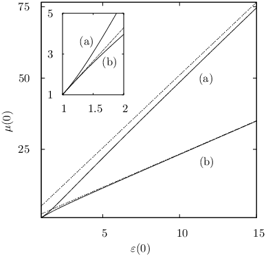
the border between the attractive and repulsive potential, i.e., , can be marked by a unique curve in the -plane [curves (a) in Fig. 2]. In particular, in the limits of weak and strong magnetodielectric properties the integral in Eq. (III.2) can be evaluated analytically. For weak magnetodielectric properties, i.e., and , the linear expansions
| (36) |
and
| (37) |
lead to
| (38) |
For strong magnetodielectric properties, i.e., and , we may approximately set, on noting that large values of are effectively suppressed in the integral in Eq. (III.2),
| (39) |
thus
| (40) |
where is the static impedance of the material. Setting in Eqs. (38) and (III.2), we obtain the asymptotic behaviour of the border curve in the two limiting cases. In particular, from Eq. (III.2) it follows that . In conclusion one can say that in the long-distance limit a repulsive vdW potential can be realized if the static magnetic properties are stronger than the static electric properties, for weak magnetodielectric properties, and for strong magnetodielectric properties.
Apart from the different distance laws, the short-distance vdW potential, Eq. (32), differs from the long-distance potential, Eq. (30), in two respects. First, the relevant coefficients and are not only determined by the static values of the permittivity and the permeability, as is seen from Eqs. (33) and (III.2), and second, Eqs. (32)–(III.2) reveal that electric and magnetic properties give rise to potentials with different distance laws and signs [ dominant (and ) if and , while and if and ]. However, although for the case of a purely magnetic plate a repulsive vdW potential proportional to is predicted, in practice the attractive term will always dominate for sufficiently small values of , because of the always existing electric properties of the plate. Hence when in the long-distance limit the potential becomes repulsive due to sufficiently strong magnetic properties, then the formation of a potential wall at intermediate distances becomes possible. It is evident that with decreasing strength of the electric properties the maximum of the wall is shifted to smaller distances while increasing in height.
In the limiting case of weak electric properties, i.e., and [recall Eqs. (28) and (29)] one can thus expect that the wall is situated within the short-distance range, so that Eqs. (32)–(III.2) can be used to determine both its position and height. From Eq. (32) we find that the wall maximum is at
| (41) |
and has a height of
| (42) |
In order to estimate the integrals in Eqs. (33) and (III.2) for the coefficients and , respectively, let us restrict our attention to the case of a two-level atom and disregard absorption ( , ). Straightforward calculation then yields ( , )
| (43) |
and
| (44) |
[ ]. Substitution of Eqs. (43) and (III.2) into Eqs. (41) and (42), respectively, eventually leads to
| (45) |
and
| (46) |
Note that consistency with the assumption of the wall being observed at short distances requires that —a condition which can be easily fulfilled for sufficiently small values of . Inspection of Eq. (III.2) shows that the height of the wall increases with increasing , decreasing , and decreasing . Since the dependence of on is much stronger than its dependendence on , the wall height increases with for given .


The distance dependence of the vdW potential, as calculated from Eq. (III.2) for a two-level atom in front of a thick magnetodielectric plate whose permittivity and permeability are modelled by Eqs. (28) and (29), respectively, is illustrated in Figs. 3 and 4. The figures reveal that the results derived above for the case where the potential wall is observed in the short-distance range remain qualitatively valid also for larger distances. So, from Fig. 3 it is seen that, for chosen values of and , the potential wall begins to form and grows in height as increases, while Fig. 4 confirms that, for chosen values of and , the height of the wall increases with . In conclusion one can say that the formation of a noticeable potential wall requires materials whose static permeability substantially exceeds the static permittivity, thereby featuring magnetic resonance frequencies as high as possible.
To study the dependence of the vdW potential on material absorption as characterized by the parameters and in Eqs. (28) and (29), we first consider the limiting behaviour of the potential for long and short distances. As the potential in the long-distance limit can be given in terms of the static permittivity and permeability, which do not depend on the absorption parameters, material absorption has no influence on the vdW force for asymptotically large distances. In contrast, absorption can affect the potential in the short-distance limit. From Eqs. (28) and (29) the inequalities
| (47) |
are seen to be valid. Combining them with Eqs. (33) and (III.2) reveals that
| (48) | |||
| (49) |
Provided that the magnetic properties of the medium are sufficiently strong to support the formation of a potential wall, these inequalities imply [cf. Eq. (32)] that increasing () leads to a shift of the wall towards smaller (larger) distances, while increasing (decreasing) its height. Thus an increase of yields a stronger repulsive potential, whereas a simultaneous increase of both absorption parameters is expected to lead to a reduction of the wall height in general. This behaviour is confirmed by the examples shown in Fig. 5, where the vdW potential of a two-level atom as given by Eq. (III.2) is displayed as a function of the distance between the atom and the plate for different values of the two absorption parameters. Note the reduced influence of absorption at large distances—in agreement with the arguments given above.

In view of left-handed materials (see, e.g., Refs. Pendry99; Smith00; Veselago68), which simultaneously exhibit negative real parts of and within some (real) frequency interval such that the real part of the refractive index becomes negative therein, the question may arise whether these materials would have an exceptional effect on the ground-state vdW force. The answer is obviously no, because the ground-state vdW potential as given by Eq. (III.2) is expressed in terms of the always positive values of the permittivity and the permeability at imaginary frequencies. Clearly, the situation may change for an atom prepared in an excited state. In such a case, the vdW potential is essentially determined by the real part of the Green tensor taken at frequencies close to the transition frequencies of the atom Buhmann04b. When there are transition frequencies that lie in frequency intervals where the material behaves left-handed, then particularities may occur.
III.3 Plate of finite thickness
Let us now consider an atom in front of a magnetodielectric plate of finite thickness [ , , , , ]. Substituting the reflection coefficients calculated from Eqs. (11) and (12) into Eq. (19), we derive ( )
| (50) |
It is obvious that the integration in Eq. (III.3) is effectively limited by the exponential factor to a circular region where . In particular, in the limit of a sufficiently thick plate, , the estimate
| (51) |
[recall Eqs. (13) and (15)] is approximately valid within (the major part of) the effective region of integration, and one may hence make the approximation in Eq. (III.3), which obviously leads back to Eq. (III.2) valid for an infinitely thick plate. On the contrary, in the limit of an asymptotically thin plate, , we find that the inequalities
| (52) |
hold in the effective region of integration, and one may hence perform a linear expansion of the integrand in Eq. (III.3) in terms of , resulting in
| (53) |
Provided that the magnetic properties are sufficiently strong, the formation of a repulsive potential wall can be also observed in the case of a genuinely magnetodielectric plate of finite thickness. Typical examples of the vdW potential obtained by numerical evaluation of Eq. (III.3) for a two-level atom are shown in Fig. 6. In the figure, the medium parameters correspond to those which have been found in Sec. III.2 to support the formation of a potential wall in the case of an infinitely thick plate. We see that the qualitative behaviour of the vdW potential is independent of the plate thickness. In particular, all curves in Fig. 6 feature a repulsive long-range potential that leads to a potential wall of finite height, the potential becoming attractive at very short distances. However, the position and height of the wall are seen to vary with the thickness of the plate. While the position of the wall shifts only slightly as the plate thickness is changed from very small to very large values, the height of the wall reacts very sensitively as the plate thickness is varied. For small values of the thickness the potential height is very small, it increases towards a maximum, and then decreases asymptotically towards the value found for the infinitely thick plate as the thickness is increased further towards very large values. It is worth noting that there is an optimal plate thickness for creating a maximum potential wall. In this case the magnitude of the plate thickness is comparable to the position of the potential maximum—a case which is realized between the two extremes of infinitely thick and infinitely thin plates.

In order to gain further insight into the competing electric and magnetic effects on the formation of an potential wall, let us study the case of an asymptotically thin plate as described by Eq. (III.3) in more detail and compare it with the case of an infinitely thick plate studied in Sec. III.2. In the long-distance limit, , Eq. (III.3) reduces to (see Appendix A)
| (54) |
where
| (55) |
while in the short-distance limit, and/or , Eq. (III.3) can be approximated by (see Appendix A)
| (56) |
where
| (57) |
and
| (58) |
In the case of an asymptotically thin plate the border between attractive and repulsive potentials is determined by the equation , because Eq. (55) reveals that
| (59) |
[cf. Eq. (35) valid for an infinitely thick plate]. Since for an asymptotically thin plate—in contrast to the infinitely thick plate—the influence of electric and magnetic properties can be completely separated into a sum of two terms, the equation can be solved analytically, leading to
| (60) |
[curves (b) in Fig. 2]. For sufficiently weak magnetodielectric properties, i.e., , , a linear expansion of the right-hand side of Eq. (60) reveals that a repulsive vdW potential can be realized if the static magnetic properties are stronger than the static electric properties by a factor , corresponding to
| (61) |
as can be seen by linearly expanding the right-hand side of Eq. (55). By comparing Eqs. (38) and (61) we realize that in the limit of weak magnetodielectric properties the border between attractive and the repulsive vdW potentials is the same for the infinitely thick plate and the asymptotically thin plate (cf. the inset in Fig. 2). This result is an immediate consequence of the fact that in this case the thick-plate potential is a linear superposition of thin-plate potentials [see Sec. III.4, Eq. (72)]. For strong magnetodielectric properties, , , the asymptotic behaviour of the right-hand side of Eq. (60) shows that the vdW potential becomes repulsive if , corresponding to
| (62) |
which follows from the corresponding asymptotic expansion of the right-hand side of Eq. (55). Hence the region in the -plane that corresponds to a repulsive vdW force is slightly increased in comparison to the infinitely thick plate.
As in the case of an infinitely thick plate, the electric and magnetic properties of the medium give rise to competing attractive and repulsive potential components, where again the attractive potential component resulting from the electric properties dominates in the limit [see Eqs. (56)–(III.3)]. This implies that for weak electric properties ( , ) a potential wall is formed in the short-distance range. From Eq. (56) it then follows that the wall is situated at
| (63) |
and has a height of
| (64) |
For a two-level atom interacting with an almost nonabsorbing ( , ) single-resonance medium exhibiting weak electric properties ( , ), the coefficients , Eq. (57), and , Eq. (III.3), can be evaluated according to
| (65) |
and
| (66) |
( ). Substitution of Eqs. (65) and (III.3) into Eqs. (63) and (64) leads to
| (67) |
(with the consistency requirement being fulfilled for sufficiently small values of ) and
| (68) |
Comparing Eqs. (III.3) and (III.3) with Eqs. (III.2) and (III.2) valid for an infinitely thick plate, we find that the dependence of both the position and the height of the potential wall on the material parameters is very similar, so that the criteria for having a noticeable potential wall given below Eq. (III.2) also apply to the case of an asymptotically thin plate. From the result that the position of the wall is almost the same in both cases it may be expected that the wall position slowly varies with the plate thickness, which is in full agreement with the exact results in Fig. 6. Further, the height of the wall is—in agreement with Fig. 6—considerably smaller for the asmyptotically thin plate. This can be seen by applying together with Eq. (III.3) in Eq. (III.3), leading to
| (69) |
the right-hand side of which is comparable to the right-hand side of Eq. (III.2). Recall that the wall height does not monotonously increase with the plate thickness in general [see Fig. 6], as could be expected from comparing the two limiting cases.
III.4 Power laws and medium-assisted correlations
Comparing the asymptotic power laws (30) and (32) obtained for an infinitely thick plate with those obtained for an asymptotically thin plate, Eqs. (54) and (56), we see that in the latter case the powers of are universally increased by one. In both cases the long-distance vdW potential follows a power law that is independent of the material properties of the plate, the sign being determined by the relative strengths of magnetic and electric properties (a purely electric plate creates an attractive vdW potential, while a purely magnetic plate gives rise to a repulsive one). Further, the short-distance results for plates of different material properties differ in both sign and leading power law (the repulsive potential created by a purely magnetic plate being weaker than the attractive potential created by a purely electric plate by two powers in the atom-plate separation). It is worth noting that a similar behaviour, i.e., the same hierarchy of power laws and the same signs have been found for the vdW force between two atoms Sucher68; Boyer69; Farina02 and for the Casimir force between two semi-infinite half-spaces Henkel04. This is illustrated in Tab. 1, where the asymptotic power laws found for an atom interacting with an infinitely thick plate, Eqs. (30) and (32), and an asymptotically thin plate, Eqs. (54) and (56), are summarized and compared to those obtainable for the interactions between two atoms or two half-spaces, respectively.
| distance | short | long | ||
|---|---|---|---|---|
| polarizability | ||||
| atom half space | ||||
| atom thin plate | ||||
| atom atom | ||||
| half space half space | ||||
For weak magnetodielectric properties, i.e., and , the similarity of the results shown in Tab. 1 can be regarded as being a consequence of the additivity of vdW-type interactions. In fact, in this case (which for a gaseous medium of given atomic species corresponds to a sufficiently dilute gas) all results of the table can be derived from the vdW interaction of two single atoms via pairwise summation. The additivity can explicitly be seen when comparing the result found for the asymptotically thin plate with that of the infinitely thick plate. Expanding the vdW potential of an infinitely thick plate, Eq. (III.2), in powers of and , we find that the leading, first-order contribution is given by
| (70) |
while the first-order contribution to the vdW potential of an asymptotically thin plate, Eq. (III.3) reads
| (71) |
Comparison of Eqs. (III.4) and (III.4) shows that to leading order in and the vdW potential of an infinitely thick plate is simply the integral over an infinite number of thin-plate vdW potentials,
| (72) |
For media with stronger magnetodielectric properties, medium-assisted correlations prevent vdW-type forces from being additive. This can be demonstrated by expanding the vdW potentials given by Eqs. (III.2) and (III.3) to second order in and , resulting in
| (73) |
and
| (74) |
respectively. The leading (second-order) correction due to medium-assisted correlations can be obtained from the vdW potential of an atom in front of two asymptotically thin plates. Physically, it can be ascribed to the process of radiation being reflected at the back (left) plate while aquiring finite phase shifts upon transmission trough the front (right) plate. The calculation yields (see Appendix B)
| (75) |
Note that the leading correction due to multiple reflections between the plates and fractional transparency of the front (right) plate are of third order in and , and are thus not relevant for the second-order correction considered here. Comparing Eqs. (III.4), (III.4), and (III.4), one can easily verify that
| (76) |
As a consequence of medium-assisted correlations the coefficients of the asymptotic power laws in Tab. 1 cannot be related via simple additivity arguments in general. However, we note from Tab. 1 that the corrections only change the coefficients of the asmptotic power laws, not the power laws themselves.
III.5 Atom between two infinitely thick plates
In Secs. III.2 and III.3 we have seen that for sufficiently strong magnetic properties a single magnetodielectric plate can feature a potential wall. This suggests that two such plates can feature a potential well, where the effect of multiple reflections between the plates must be taken into account. Let us consider the simplest case of an atom placed between two identical infinitely thick magnetodielectric plates which are separated by a distance [ , , , , ]. From Eq. (II) together with Eqs. (11)–(14) it then follows that ( )
| (77) |
where the coefficients
| (78) | ||||
| (79) |
describe the effect of multiple reflections of radiation between the two plates, as can be seen from the expansion
| (80) |
As a consequence of multiple reflections the vdW potential of an atom between the two plates, Eq. (III.5), can be different from the sum of two single-plate potentials, Eq. (III.2).

Examples of the vdW potential for a two-level atom between two identical infinitely thick magnetodieletric plates as given by Eq. (III.5) are plotted in Figs. 7 and 8. In the case of the parameters chosen in Fig. 7 multiple reflections are negligible, so that the potentials effectively reduce to sums of single-plate potentials. This obviously results from the smallness of the relevant reflection coefficients together with the relatively large distance between the plates. From Eqs. (11) and (12) one can easily verify that
| (81) | ||||
| (82) |
Hence in the case of the parameters in Fig. 7(a) we have , . In order to demonstrate the effect of multiple reflections, in Fig. 8 we have (artificially) increased the reflection coeffiecients, so that almost perfect reflection is realized ( , ), and reduced the plate separation.

It is seen that multiple reflections lead to a slight lowering of the vdW potential in the region near the midpoint between the two plates.
IV Summary and Conclusions
We have studied the problem of the van der Waals force acting on a ground-state atom in the presence of planar, dispersing, and absorbing magnetodielectric bodies. Considering an arbitrary planar multilayer system and restricting our attention to the lowest (nonvanishing) order of perturbation theory, we have given a general expression for the vdW potential. The effect of the multilayer system is expressed in terms of generalized reflection coefficients, which on their part are determined, inter alia, by the (complex) permittivities and permeabilities of the layers. Applying the formula to the cases of an atom being in front of a magnetodielectric plate and between two such plates, we have placed special emphasis on the competing attractive and repulsive force components associated with the electric and magnetic matter properties, respectively. Both numerical and analytical results are given, the latter referring to some limiting cases such as the asymptotic behaviour of the potential for thick and thin plates in the long- and short-distance limits.
In contrast to the well-known attractive vdW force generated by a purely dielectric plate, a purely magnetic plate leads to a repulsive force. In the case of genuinely magnetodielectric material, the influence of the magnetic properties can thus considerably reduce the strength of the vdW force and—for sufficiently strong magnetic properties—even create a repulsive potential wall of finite height. The numerical results show that the height of such a potential wall sensitively depends not only on the relative strengths of the electric and magnetic properties, but also on the thickness of the plate. In particular, they suggest that the maximum height is realized in the case when the thickness of the plate is comparable to the distance of the potential maximum from the plate. Comparing the results obtained for an infinitely thick plate with those found for an asymptotically thin plate, we have found striking similarities which for weakly magnetodielectric media can be explained by the additivity of vdW potentials. Moreover, we have explicitly demonstrated how medium-assisted correlations lead to a breakdown of additivity for media with stronger magnetodielectric properties. For an atom being situated between two magnetodielectric plates each of which features a potential barrier, a potential well of finite depth can be formed. If the plates possess a sufficiently high reflectivity while being relatively close together multiple reflections can prevent the resulting potential from being simply the additive superposition of the two single-plate potentials.
The results show that the advent of artificially made materials with controllable magnetodielectric properties will offer novel possibilities of realizing vdW potentials on demand. The provided analysis of typical effects relevant for controlling the vdW force in the case of one and two magnetodielectric plates—namely the competition between electric and magnetic properties of the material in the formation of the potential, material absorption, plate thickness, and multiple reflections—can of course be extended to more complex multilayer systems by further evaluating the general formula for the vdW potential of a ground-state atom in planar multilayer systems.
Acknowledgements.
This work was supported by the Deutsche Forschungsgemeinschaft. We thank Ho Trung Dung and J.B. Pendry for valuable discussions. S.Y.B. is grateful for having been granted a Thüringer Landesgraduiertenstipendium and acknowledges support by the E.W. Kuhlmann-Foundation. T.K. is grateful for being member of Graduiertenkolleg 567, which is funded by the Deutsche Forschungsgemeinschaft and the Government of Mecklenburg-Vorpommern.Appendix A Long- and short-distance limits
The long-distance (short-distance) limit corresponds to separations between the atom and the multilayer system which are much greater (smaller) than the wavelenghts corresponding to typical frequencies of the atom and the multilayer system. To obtain approximate results for the two limiting cases, let us analyze the -integrals in Eqs. (III.2) and (III.3) in a little more detail and begin with the long-distance limit, i.e.,
| (83) |
where is the lowest atomic transition frequency, and is the lowest medium resonance frequency. For convenience, we introduce the new integration variable and transform the integral according to
| (84) |
where has to be replaced according to
| (85) |
Inspection of Eqs. (III.2) and (III.3) together with Eq. (A) reveals that the frequency interval giving the main contribution to the respective -integral is determined by a set of effective cutoff functions, namely
| (86) |
| (87) |
which enter via the atomic polarizability, cf. Eq. (3), and
| (88) | ||||
| (89) |
which enter via and , cf. Eqs. (28) and (29). The cutoff functions obviously give their main contributions in regions, where
| (90) | ||||||
| (91) | ||||||
| (92) | ||||||
| (93) |
Combining Eq. (90) with Eq. (83), we find that the function effectively limits the -integration to a region where
| (94) | ||||
| (95) | ||||
| (96) |
Performing a leading-order expansion of the integrands in Eqs. (III.2) and (III.3) in terms of the small quantities , , and , we may set
| (97) |
Combining Eqs. (A), (85), and (97) with Eq. (III.2) and Eq. (III.3), repectively, and evaluating the remaining -integrals we arrive at Eq. (30) [together with Eq. (III.2)] and Eq. (54) [together with Eq. (55)].
The short-distance limit, on the contrary, is defined by
| (98) |
where is the highest inneratomic transition frequency, is the highest medium resonance frequency, and is the static refractive index of the medium. Again, it is convenient to change the integration variables in Eqs. (III.2) and (III.3), but now we transform according to
| (99) |
where has to be replaced according to
| (100) |
Combining Eqs. (91)–(93) with Eq. (98) reveals that the functions , , and limit the -integration to a region where
| (101) |
and/or
| (102) |
A valid approximation to the -integrals in Eqs. (III.2) and (III.3) can hence be obtained by performing a Taylor exansion in . To that end, we apply the transformation (A) to Eqs. (III.2) and (III.3), respectively, retain only the leading-order terms in (which after carrying out the -integral will yield the leading-order terms in ) and obtain
| (103) |
and
| (104) |
After evaluating the -integrals and keeping only the leading-order terms in [note that Eqs. (91)–(93) together with Eq. (98) imply ], Eq. (A) and Eq. (A), respectively, result in Eq. (32) [together with Eqs. (33) and (III.2)] and Eq. (56) [together with Eqs. (57) and (III.3)].
Appendix B Derivation of Eq. III.4
In order to derive Eq. (III.4), we consider the vdW potential of two plates of thickness , which are separated by a distance [ , , , , , , ]. We assume both plates to be asymptotically thin, , , so that the inequalities , ( , ) are valid, cf. Eq. (III.3). Use of Eqs. (11) and (12) for and , followed by a linear expansion in terms of , yields
| (105) | ||||
| (106) |
while use of the same equations for and together with leads to, upon linearly expanding in terms of ,
| (107) | ||||
| (108) |
Substituting Eqs. (107) and (108) into Eqs. (B) and (B), respectively, and neglecting terms which are quadratic in , we arrive at
| (109) | ||||
| (110) |
The leading correction due to medium correlations can be extracted from Eqs. (B) and (B) by retaining only the two-plate contribution, i.e., the term which is linear in both and . We expand the result up to linear order in , , , and , thereby discarding terms which are independent of and , leading to
| (111) | ||||
| (112) |
where we have set , , and . Substitution of Eqs. (B) and (B) into Eq. (19) leads to Eq. (III.4). In order to see that this leading correction corresponds to the process of radiation being reflected at the back (left) plate while aquiring finite phase shifts upon transmission trough the front (right) plate, we note that up to linear order in , , and , the terms in square brackets in Eqs. (B) and (B) are equal to the phase factor , as can be easily verified by recalling Eq. (13):
| (113) |
similar for Eq. (B).
References
- (1) C. I. Sukenik, M. G. Boshier, D. Cho, V. Sandoghdar, and E. A. Hinds, Phys. Rev. Lett. 70, 5, 560 (1993); A. Anderson, S. Haroche, E. A. Hinds, W. Jhe, and D. Meschede, Phys. Rev. A 37, 9, 3594 (1988).
- (2) F. Shimizu, Phys. Rev. Lett. 86, 6, 987 (2001); F. Shimizu and J.-i. Fujita, ibid. 88, 12, 123201 (2002); V. Druzhinina and M. DeKieviet, Phys. Rev. Lett. 91, 193202 (2003).
- (3) V. Sandoghdar, C. I. Sukenik, E. A. Hinds, and S. Haroche, Phys. Rev. Lett. 68, 23, 3432 (1992); M. Marrocco, M. Weidinger, R. T. Sang, and H. Walther, Phys. Rev. Lett. 81, 26, 5784 (1998); M. A. Wilson, P. Bushev, J. Eschner, F. Schmidt-Kaler, C. Becher, R. Blatt, and U. Dorner, Phys, Rev. Lett. 91, 21, 213602 (2003); P. Bushev, A. Wilson, J. Eschner, C. Raab, F. Schmidt-Kaler, C. Becher, and R. Blatt, ibid. 92, 22, 223602 (2004).
- (4) M. Oria, M. Chevrollier, D. Bloch, M. Fichet, and M. Ducloy, Europhy. Lett. 14, 6, 527 (1991); M. Chevrollier, D. Bloch, G. Rahmat, and M. Ducloy, Opt. Lett. 16, 23, 1879 (1991); M. Chevrollier, M. Fichet, M. Oria, G. Rahmat, D. Bloch, and M. Ducloy, J. Phys. II France 2, 631 (1992); M. Gorris-Neveux, P. Monnot, M. Fichet, M. Ducloy, and R. Barbé, J. C. Keller, Opt. Commun. 134, 85 (1997), H. Failache, S. Saltiel, M. Fichet, D. Bloch, and M. Ducloy, Phys. Rev. Lett. 83, 26, 5467 (1999); M. Boustimi, B. Viaris de Lesegno, J. Baudon, J. Robert, and M. Ducloy, Phys. Rev. Lett. 86, 13, 2766 (2001); H. Failache, S. Saltiel, M. Fichet, D. Bloch, and M. Ducloy, Eur. Phys. J. D 23, 237 (2003).
- (5) J.E. Lennard-Jones, Trans. Farad. Soc. 28, 333 (1932); see also J. Bardeen, Phys. Rev. 58, 727 (1940); H. Margenau and W.G. Pollard, Phys. Rev. 60, 128 (1941).
- (6) H.B.G. Casimir and D. Polder, Phys. Rev. 73, 360 (1948).
- (7) G. Barton, J. Phys. B, 7, 16, 2134 (1974); D. Meschede, W. Jhe, and E. A. Hinds, Phys. Rev. A 41, 3, 1587 (1990).
- (8) T. Nakajima, P. Lambropoulos, and H. Walther, Phys. Rev. A 56, 6, 5100 (1997).
- (9) Y. Tikochinsky and L. Spruch, Phys. Rev. A 48, 6, 4223 (1993).
- (10) F. Zhou and L. Spruch, Phys. Rev. A 52, 297 (1995).
- (11) S.Y. Buhmann, Ho Trung Dung, and D.-G. Welsch, J. Opt. B: Quantum Semicl. Opt. 6, 127 (2004).
- (12) S.Y. Buhmann, L. Knöll, D.-G. Welsch, and Ho Trung Dung, Phys. Rev. A 70, 052117 (2004).
- (13) A.D. McLachlan, Proc. R. Soc. London Ser. A 271, 387 (1963).
- (14) A.D. McLachlan, Mol. Phys. 7, 381 (1963); G. S. Argawal, Phys. Rev. A 11, 1, 243 (1975).
- (15) J.M. Wylie and J.E. Sipe, Phys. Rev. A 30, 1185 (1984).
- (16) J.M. Wylie and J.E. Sipe, Phys. Rev. A 32, 2030 (1985).
- (17) C. Henkel, V. Sandoghdar, Opt. Commun. 158, 250 (1998).
- (18) A.D. McLachlan, Proc. R. Soc. London Ser. A 274, 80 (1963); C. Henkel, K. Joulain, J.-P. Mulet, J.J. Greffet, J. Opt. A: Pure Appl. Opt. 4, 109 (2002).
- (19) M.-P. Gorza, S. Saltiel, H. Failache, M. Ducloy, Eur. Phys. J. D 15, 113 (2001).
- (20) S. Kryszewski, Mol. Phys. 78, 5, 1225 (1993).
- (21) M.J. Renne, Physica 53, 193 (1971).
- (22) T.H. Boyer, Phys. Rev. A 5, 4, 1799 (1972); 6, 1, 314 (1972); 7, 6, 1832 (1973).
- (23) M.J. Renne, Physica 56, 124 (1971).
- (24) C. Mavroyannis, Mol. Phys. 6, 593 (1963).
- (25) J. Schwinger, L.L. DeRaad, and K.A. Milton, Ann. Phys. (New York) 115, 1 (1978); see also P. W. Milonni and M.-L. Shih, Phys. Rev. A 45, 4241 (1992).
- (26) M. Fichet, F. Schuller, D. Bloch, and M. Ducloy, Phyys. Rev. A 51, 2, 1553 (1995).
- (27) J.-Y. Courtois, J.-M. Courty, J.C. Mertz, Phys. Rev. A 53, 1862 (1996).
- (28) J.B. Pendry, A. J. Holden, D.J. Robbins, and W.J. Stewart, IEEE Trans. Microwave Theory Tech. 47, 11, 2075 (1999).
- (29) D.R. Smith, W. J. Padilla, D.C. Vier, S.C. Nemat-Nasser, and S. Schultz, Phys. Rev. Lett. 84, 18, 4184 (2000).
- (30) G. Feinberg and J. Sucher, Phys. Rev. A 2, 6, 2395 (1970); for an extension see E. Lubkin, Phys. Rev. A 4, 1, 416 (1971).
- (31) G. Feinberg and J. Sucher, J. Chem. Phys. 48, 7, 3333 (1968).
- (32) T.H. Boyer, Phys. Rev. 180, 1, 19 (1969).
- (33) C. Farina, F.C. Santos, and A.C. Tort, J. Phys. A 35, 2477 (2002); Am. J. Phys. 70, 4, 421 (2002).
- (34) T.H. Boyer, Phys. Rev. A 9, 5, 2078 (1974); V. Hushwater, Am. J. Phys. 65, 5, 381 (1997); M. Schaden and L. Spruch, Phys. Rev. A 58, 2, 935 (1998); M.V. Cougo-Pinto, C. Farina, and A. Tenório, Braz. J. Phys. 29, 371 (1999); F.C. Santos, A. Tenório, and A.C. Tort, Phys. Rev. D 60, 105022 (1999).
- (35) C. Henkel and K. Joulain, e-print quant-ph/0407153.
- (36) O. Kenneth, I. Klich, A. Mann, and M. Revzen, Phys. Rev. Lett. 89, 3, 033001 (2002); see also E. Buks and M. Roukes, Nature 419, 119 (2002).
- (37) M.S. Tomǎs, e-print quant-ph/0410057; for the well-known case of purely dielectric plates cf., e.g., E. M. Lishitz, JETP (USSR) 29, 94 (1955); C. Raabe, L. Knöll, and D.-G. Welsch, Phys. Rev. A 68, 033810 (2003).
- (38) D. Iannuzzi and F. Capasso, Phys. Rev. Lett. 91, 2, 029101 (2003); for a reply see O. Kenneth, I. Klich, A. Mann, and M. Revzen, Phys. Rev. Lett. 91, 2, 029102 (2003).
- (39) W.C. Chew, Waves and Fields in Inhomogeneous Media (IEEE Press, New York, 1995), Secs. 2.1.3, 2.1.4, and 7.4.2.
- (40) K.P. Thakur and W.S. Holmes, IEEE Trans. Microwave Theory Tech. 52, 1, 76 (2004).
- (41) V.G. Veselago, Sov. Phys. Usp. 10, 509 (1968).