Ghost Interference and Quantum Erasure

Imagine the slit to be a position filter - it allows portions of the wavefunction in front of the slit, to go through. Let us assume that what emerges from a slit is a localized Gaussian packet, whose width is the width of the slit. So, if the two slits are A and B, the packets which pass through will be, say, $|\phi_{A}(y_{1})\rangle$ and $|\phi_{B}(y_{1})\rangle$, respectively.

The entangled state at time $t_{0}$, $|\Psi(y_{1},y_{2},t_{0})\rangle$, can then be expanded in terms of components parallel to $|\phi_{A}(y_{1})\rangle$ and $|\phi_{B}(y_{1})\rangle$, and orthogonal to those. We can write

$$|\Psi(y_{1},y_{2},t_{0})\rangle=|\phi_{A}\rangle\langle\phi_{A}|\Psi\rangle+|\phi_{B}\rangle\langle\phi_{B}|\Psi\rangle+|\chi\rangle\langle\chi|\Psi\rangle.$$

(7)

where $|\chi(y_{1})\rangle$ represents rest of the states in the Hilbert space, orthogonal to $|\phi_{A}(y_{1})\rangle$ and $|\phi_{B}(y_{1})\rangle$. So, the states of particle 2 that one has to calculate are

	$\displaystyle\psi_{A}(y_{2})$	$\displaystyle=$	$\displaystyle\langle\phi_{A}(y_{1})|\Psi(y_{1},y_{2},t_{0})\rangle$
	$\displaystyle\psi_{B}(y_{2})$	$\displaystyle=$	$\displaystyle\langle\phi_{B}(y_{1})|\Psi(y_{1},y_{2},t_{0})\rangle$
	$\displaystyle\psi_{\chi}(y_{2})$	$\displaystyle=$	$\displaystyle\langle\chi(y_{1})|\Psi(y_{1},y_{2},t_{0})\rangle$		(8)

So, the state we get after particle 1 crosses the double-slit is:

$$|\Psi(y_{1},y_{2})\rangle=|\phi_{A}\rangle|\psi_{A}\rangle+|\phi_{B}\rangle|\psi_{B}\rangle+|\chi\rangle|\Psi_{\chi}\rangle,$$

(9)

where $|\phi_{A}\rangle$ and $|\phi_{B}\rangle$ are states of particle 1, and $|\psi_{A}\rangle$ and $|\psi_{B}\rangle$ are states of particle 2. The first two terms represent the amplitudes of particle 1 passing through the slits, and the last term represents the amplitude of it getting reflected/blocked. Because of the linearity of Schrödinger equation, these two pieces of the wavefunction will evolve independently, without affecting each other. Because we are interested only in situations where particle 1 passes through the slit, we might as well throw away the term which represents particle 1 not passing through the slits. If we do that, we have to normalize the remaining part of the wavefunction, which looks like

$$|\Psi(y_{1},y_{2})\rangle={1\over C}(|\phi_{A}\rangle|\psi_{A}\rangle+|\phi_{B}\rangle|\psi_{B}\rangle),$$

(10)

where $C=\sqrt{\langle\psi_{A}|\psi_{A}\rangle+\langle\psi_{B}|\psi_{B}\rangle}$.

In the following, we assume that $|\phi_{A}\rangle$, $|\phi_{B}\rangle$, are Gaussian functions in space:

$$\phi_{A}(y_{1})={1\over(\pi/2)^{1/4}\sqrt{\epsilon}}e^{-(y_{1}-y_{0})^{2}/\epsilon^{2}},~~~~~\phi_{B}(y_{1})={1\over(\pi/2)^{1/4}\sqrt{\epsilon}}e^{-(y_{1}+y_{0})^{2}/\epsilon^{2}},$$

(11)

where $\pm y_{0}$ is the y-position of slit A and B, respectively, and $\epsilon$ their widths. Thus, the distance between the two slits is $2y_{0}$.

Using (8) and (6), wavefunctions $|\psi_{A}\rangle$, $|\psi_{B}\rangle$ can be calculated, which, after normalization, have the form

$$\psi_{A}(y_{2})=C_{2}e^{-{(y_{2}-y_{0}^{\prime})^{2}\over\Gamma^{2}}},~~~\psi_{B}(y_{2})=C_{2}e^{-{(y_{2}+y_{0}^{\prime})^{2}\over\Gamma^{2}}},$$

(12)

where $C_{2}={1\over(\pi/2)^{1/4}\sqrt{\Gamma}}$,

$$y_{0}^{\prime}={y_{0}\over{4\Omega^{2}\sigma^{2}/\hbar^{2}+1\over 4\Omega^{2}\sigma^{2}/\hbar^{2}-1}+{4\epsilon^{2}\over 4\Omega^{2}-\hbar^{2}/\sigma^{2}}},$$

(13)

and

$$\Gamma^{2}=\frac{{\hbar^{2}\over\sigma^{2}}(1+{\epsilon^{2}+2i\hbar t_{0}/m\over 4\Omega^{2}})+\epsilon^{2}+2i\hbar t_{0}/m}{1+{\epsilon^{2}+2i\hbar t_{0}/m\over\Omega^{2}}+{\hbar^{2}\over 4\Omega^{2}\sigma^{2}}}+{2i\hbar t_{0}\over m}.$$

(14)

The state which emerges from the double slit, now assumes the form

$$\Psi_{r}(y_{1},y_{2})=C_{1}e^{-(y_{1}-y_{0})^{2}/\epsilon^{2}}C_{2}e^{-{(y_{2}-y_{0}^{\prime})^{2}\over\Gamma^{2}}}+C_{1}e^{-(y_{1}+y_{0})^{2}/\epsilon^{2}}C_{2}e^{-{(y_{2}+y_{0}^{\prime})^{2}\over\Gamma^{2}}},$$

(15)

where $C_{1}=\left({2\epsilon^{2}\over\pi}\right)^{1/4}$ Equation (15) represents two wave-packets of particle 1, of width $\epsilon$, and localized at $\pm y_{0}$, entangled with two wave-packets of particle 2, of width ${\sqrt{2}|\Gamma|^{2}\over\sqrt{\Gamma^{2}+\Gamma^{*2}}}$, localized at $\pm y_{0}^{\prime}$.

The state (15) represents particle 1 passing through a double-slit. But if $|\psi_{A}\rangle$ and $|\psi_{B}\rangle$ are orthogonal, the amplitudes of particle 1 passing through the two slits are correlated with two distinguishable states of particle 2. Hence, in principle, a measurement on particle 2 can reveal which slit particle 1 passed through. According to the Complementarity principle, no interference can be observed in such a situation. So, no interference can be seen in particle 1 because particle 2 carries the “which-way” information about particle 1. This is the fundamental reason for photon 1 not showing interference in the ghost interference experiment, and not its large momentum spread.

From (15) one can see that the state of particle 2 also involves two spatially separated, localized Gaussians, correlated with states of particle 1. So, because of entanglement, particle 2 also behaves as if it has passed through a double-slit of separation $2y_{0}^{\prime}$. In other words, because of entanglement, particle 1 passing through the double-slit, creates a virtual double-slit for particle 2. This view is in agreement with the observed optical imaging by means of entangled photons [9]. It appears natural that particle 2, passing through this virtual double-slit, should show an interference pattern. However, this can happen only when the wave-packets overlap, after evolving in time.

Before reaching detector D2, particle 2 evolves for a time $t$. The time evolution, governed by (5), transforms the state (15) to

	$\displaystyle\Psi_{r}(y_{1},y_{2},t)$	$\displaystyle=$	$\displaystyle C_{1}(t)e^{-{(y_{1}-y_{0})^{2}\over\epsilon^{2}+2i\hbar t/m}}C_{2}(t)e^{-{(y_{2}-y_{0}^{\prime})^{2}\over\Gamma^{2}+2i\hbar t/m}}$
			$\displaystyle+C_{1}(t)e^{-{(y_{1}+y_{0})^{2}\over\epsilon^{2}+2i\hbar t/m}}C_{2}(t)e^{-{(y_{2}+y_{0}^{\prime})^{2}\over\Gamma^{2}+2i\hbar t/m}},$

where

$$C_{1}(t)={1\over(\pi/2)^{1/4}\sqrt{\epsilon+2i\hbar t/m\epsilon}},~~~C_{2}(t)={1\over(\pi/2)^{1/4}\sqrt{\Gamma+2i\hbar t/m\Gamma}}.$$

(17)

Before proceeding further, we need to simplify the expression for $\Gamma$. We assume the spatial extent of the wave-function $\Psi(y_{1},y_{2})$ to be large, namely, $\Omega\gg\epsilon$ and $\Omega\gg\hbar/\sigma$. In this limit,

$$\Gamma^{2}\approx\gamma^{2}+4i\hbar t_{0}/m,$$

(18)

where $\gamma^{2}=\epsilon^{2}+\hbar^{2}/\sigma^{2}$ and $y_{0}^{\prime}\approx y_{0}$. We are now in a position to calculate the probability of finding particle 1 at $y_{1}$ and particle 2 at $y_{2}$. This is given by

	$\displaystyle|\Psi_{r}(y_{1},y_{2},t)|^{2}$	$\displaystyle=$	$\displaystyle|C_{1}(t)C_{2}(t)|^{2}\times\left(\exp\left[{-{2(y_{1}-y_{0})^{2}\over\epsilon^{2}+({2\hbar t\over m\epsilon})^{2}}}-{2(y_{2}-y_{0}^{\prime})^{2}\over\gamma^{2}+({2\hbar(t+2t_{0})\over m\gamma})^{2}}\right]\right.$
			$\displaystyle+\exp\left[{-{2(y_{1}+y_{0})^{2}\over\epsilon^{2}+({2\hbar t\over m\epsilon})^{2}}}{-{2(y_{2}+y_{0}^{\prime})^{2}\over\gamma^{2}+({2\hbar(t+2t_{0})\over m\gamma})^{2}}}\right]$
			$\displaystyle+\left.\exp\left[{-{2(y_{1}^{2}+y_{0}^{2})\over\epsilon^{2}+({2\hbar t\over m\epsilon})^{2}}-{2(y_{2}^{2}+y_{0}^{\prime 2})\over\gamma^{2}+({2\hbar(t+2t_{0})\over m\gamma})^{2}}}\right]\times 2\cos\left[\theta_{1}y_{1}+\theta_{2}y_{2}\right]\right),$

where

$$\theta_{1}={8y_{0}\hbar t/m\over\epsilon^{4}+4\hbar^{2}t^{2}/m^{2}},~~~\theta_{2}={8y_{0}\hbar(t+2t_{0})/m\over\gamma^{4}+4\hbar^{2}(t+2t_{0})^{2}/m^{2}}.$$

(20)

We can now make contact with the ghost interference experiment, where detector D1 is kept fixed and detector D2 is scanned along the y-axis. If we fix $y_{1}$, the cosine term in (2.2) represents oscillations as a function of $y_{2}$. This implies that if particle 2 is detected in coincidence with particle 1 being detected at a fixed position $y_{1}$, then it shows interference. This is ghost interference. In the expression for $\theta_{2}$, $\gamma$ is a measure of the width of the virtual slits created because of particle 1 passing through the double-slit. So, it is clear that the ghost interference is an effect due to the virtual slits formed for particle 2, because of a measurement on the spatially separated particle 1, with which it is correlated due to entanglement.

Coming back to ghost interference, one might wonder that if the virtual slits are created by particle 1 passing through the double-slit, what is the need for fixing detector D1 and doing a coincident count. The answer is, particle 1 carries which-way information about particle 2. Meaning, particle 1 can be potentially detected in such a manner that would tell us which virtual slit, A or B, did particle 2 pass through. And Bohr’s complementarity principle tells us that in such a situation, interference cannot be observed [10]. By detecting particle 1 at a fixed position, where contributions from both the slits are present, we add the two contributions, and thus erase the information about which slit particle 1, and particle 2, passed through. Once the which-way information is erased, the interference can come back, and it does. So, the mechanism behind the appearance of ghost interference is two-fold. Quantum entanglement of the two particles leads to the creation of a virtual double-slit for particle 2, and quantum erasure [11] of the which-way information (again via entanglement) leads to appearance of interference from the virtual double-slit.

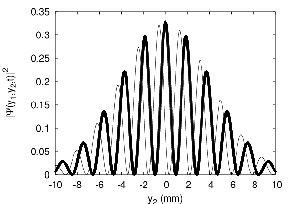
Scully Englert and Walther proposed a setup for quantum eraser, where the which-way detector is a two-state system [12]. Quantum erasure is performed when the particles are detected in coincidence with one of the two special states of the which-way detector, which do not discriminate between the two paths of the particle. Corresponding to these two states of the which-way detector, two interference patterns are obtained which are complementary, meaning, they add up to give no interference. In the case of ghost interference, the role of the states carrying which-way information is played by the position of particle 1, namely $y_{1}$, which is a continuous variable. Detection of particle 1 by a fixed detector D1 destroys the which-way information carried by it. Thus D1 acts as an eraser of the which-way information. From (2.2), one can see that for a fixed $y_{1}$, the term $\theta_{1}y_{1}$ acts as an extra phase for the cosine function in $y_{2}$. Thus, the whole interference pattern is shifted, depending on the position of D1 (see Fig. 2), so that when all the D1 positions are added, it results in the destruction of the interference pattern. This is the reason why, in Strekalov et al.’s experiment, no interference for photon 2 is observed without coincident counting with a fixed D1.

One must have already noticed something strange about (2.2), namely, in the terms for particle 2, the time which appears is $t+2t_{0}$ as opposed to just $t$ for particle 1. In the actual experiment, time is not what is the meaningful quantity - it is the distance the particle travels, that is relevant. Let us translate our results to the situation where one just measures the distance. For that we assume that particle 2 travels along the x-axis, with a momentum $p$. In time $t_{0}$, both particle 1 and particle 2 travel a distance $L_{2}$. During time $t$, particle 1 travels a distance $L_{1}$ to reach D1, and particle 2 travels the same distance to reach D2. So, the time $t+2t_{0}$ corresponds to the distance between the double-slit and D2, that is, $D$. Using this strategy, we can write $\hbar(t+2t_{0})/m=\hbar v(t+2t_{0})/p=\lambda_{d}v(t+2t_{0})/2\pi=\lambda_{d}D/2\pi$, where $\lambda_{d}$ is the d’Broglie wavelength of the particle and $v$ its velocity. The expression $\lambda_{d}D/2\pi$ will also hold for a photon provided, one uses the wavelength of the photon in place of $\lambda_{d}$. The probability of coincident click of D1 and D2 is given by $P(y_{1},y_{2})=|\Psi_{r}(y_{1},y_{2},t)|^{2}$, which has the following form

	$\displaystyle P(y_{1},y_{2})$	$\displaystyle=$	$\displaystyle|C_{1}(t)C_{2}(t)|^{2}\left(\exp\left[-{2(y_{1}-y_{0})^{2}\over\epsilon^{2}+(\lambda_{d}L_{1}/\pi\epsilon)^{2}}-{2(y_{2}-y_{0})^{2}\over\gamma^{2}+(\lambda_{d}D/\pi\gamma)^{2}}\right]\right.$
		$\displaystyle+$	$\displaystyle\exp\left[-{2(y_{1}+y_{0})^{2}\over\epsilon^{2}+(\lambda_{d}L_{1}/m\epsilon)^{2}}-{2(y_{2}+y_{0})^{2}\over\gamma^{2}+(\lambda_{d}D/\pi\gamma)^{2}}\right]$
		$\displaystyle+$	$\displaystyle\exp\left[-{2(y_{1}^{2}+y_{0}^{2})\over\epsilon^{2}+(\lambda_{d}L_{1}/\pi\epsilon)^{2}}-{2(y_{2}^{2}+y_{0}^{2})\over\gamma^{2}+(\lambda_{d}D/\pi\gamma)^{2}}\right]\times 2\cos\left[\theta_{1}y_{1}+\theta_{2}y_{2}\right]\left.\right),$

where $\theta_{1}={4y_{0}\lambda_{d}L_{1}/\pi\over\epsilon^{4}+\lambda_{d}^{2}L_{1}^{2}/\pi^{2}}$, $\theta_{2}={4y_{0}\lambda_{d}D/\pi\over\gamma^{4}+\lambda_{d}^{2}D^{2}/\pi^{2}}$. Equation (2.4) tells us that the fringe width of the pattern for particle 2 is given by

$$w_{2}={2\pi\over\theta_{2}}=2\pi{\lambda_{d}^{2}D^{2}/4\pi^{2}+\gamma^{4}/4\over 2y_{0}\lambda_{d}D/2\pi}={\lambda_{d}D\over 2y_{0}}+{\gamma^{4}\pi\over 4y_{0}\lambda_{d}D}$$

(22)

For $\gamma^{2}\ll\lambda_{d}D$, we get the familiar Young’s double-slit interference formula,

$$w_{2}\approx{\lambda_{d}D\over 2y_{0}},$$

(23)

where $2y_{0}$ is the separation between the slits. Notice that $D$ is the strange distance from the detector D2, right through the source, to the double slit (see Fig. 1). Particle 2 never passes through the region between the source and the double-slit. This is exactly what was observed in Strekalov et al.’s experiment. Although the virtual double-slit for particle 2 comes into being only after particle 2 travels a distance $L_{2}$ from the source, the particle carries with itself the phase information of its evolution from the source for the time $t_{0}$. Because of coincident counting, the change in phase because of the evolution of particle 1 is added to that of particle 2, and it appears as if particle 2 traveled a distance $2L_{2}$, which is double the actually traveled distance. So, we see that although the virtual double-slit comes into being after particle 1 enters the real double-slit, for all practical purposes, it appears as if the virtual double-slit is located exactly at the real double-slit, behind the source. We should also mention that for values of various parameters corresponding to Strekalov et al.’s experiment, their results are faithfully reproduced by (2.4).

Eqn. (2.4) is reasonably symmetric in $y_{1}$ and $y_{2}$, except for the difference in the widths of the real and virtual slits, and $L_{1}$ appearing for particle 1, and $D$ appearing for particle 2. It is but natural to expect that by fixing D2 at some $y_{2}$, and counting particle 1 in coincidence with D2, should show an interference. The fringe width of the interference pattern is given by

$$w_{1}={2\pi\over\theta_{1}}=2\pi{\lambda_{d}^{2}L_{1}^{2}/4\pi^{2}+\epsilon^{4}/4\over 2y_{0}\lambda_{d}L_{1}/2\pi}\approx{\lambda_{d}L_{1}\over 2y_{0}}$$

(24)

The fringe width is exactly what one would expect from a conventional first order interference. In this sense, this pattern is not as spectacular as that for particle 2. The term $\theta_{2}y_{2}$ now acts as an additional phase of the cosine, and this leads to a shift in the interference pattern for particle 1 if the position of D2 is changed.

Kim et al. [13] performed an experiment which, in the context of the experiment described here, would amount to looking for interference in particle 1, by erasing the which-way information carried by particle 2. They demonstrate that the two-slit interference is recovered once the which-way information is erased. However, they go further than that. They not only actually acquire which-way information for each passing particle, which does not happen in the experiment described here, they demonstrate that which-way information can be erased much after the particle has been physically detected, and still leads to recovery of interference. The physical interpretation of such “delayed-choice” quantum erasure has been much debated upon [14, 15, 16].

References

- [1] D. V. Strekalov, A. V. Sergienko, D. N. Klyshko, and Y. H. Shih, Phys. Rev. Lett. 74 (1995), 3600.
- [2] M. D’Angelo, Y-H. Kim, S. P. Kulik and Y. Shih, Phys. Rev. Lett. 92 (2004), 233601.
- [3] S. Thanvanthri and M. H. Rubin, Phys. Rev. A 70 (2004), 063811.
- [4] Y-H. Zhai, X-H. Chen, D. Zhang, L-A. Wu, Phys. Rev. A 72 (2005), 043805.
- [5] L. Jie, C. Jing, Chinese Phys. Lett. 28 (2011), 094203
- [6] R. Christanell, W. Weinfurter, and A. Zeilinger, The Technical Digest of the European Quantum Electronic Conference, EQEC‘93, Florence, 1993 (unpublished), p. 872.
- [7] I. Neder, M. Heiblum, D. Mahalu, V. Umansky, Phys. Rev. Lett. 98 (2007), 036803.
- [8] L. Mandel and E. Wolf, Optical Coherence and Quantum Optics (Cambridge, University Press, 1995).
- [9] T.B. Pittman, Y.H. Shih, D.V. Strekalov, A.V. Sergienko, Phys. Rev. A, 52 (1995), R3429.
- [10] N. Bohr, Nature 121 (1928), 580.
- [11] M. O. Scully and K. Drühl, Phys. Rev. A 25 (1982), 2208.
- [12] M. O. Scully, B.-G. Englert and H. Walther, Nature (London) 351 (1991), 111.
- [13] Y-H Kim, R. Yu, S.P. Kulik, Y. Shih, M.O. Scully, Phys. Rev. Lett. 84 (2000), 1-5.
- [14] J.A. Wheeler, pp. 182-213 in Quantum Theory and Measurement, J.A. Wheeler and W.H. Zurek edit., (Princeton University Press, 1984).
- [15] B.-G. Englert, M. O. Scully and H. Walther, Am. J. Phys. 67, 325 (1999).
- [16] U. Mohrhoff, Am. J. Phys. 67, 330 (1999).