Geometry of an adiabatic passage at a level crossing
Abstract
We discuss adiabatic quantum phenomena at a level crossing. Given a path in the parameter space which passes through a degeneracy point, we find a criterion which determines whether the adiabaticity condition can be satisfied. For paths that can be traversed adiabatically we also derive a differential equation which specifies the time dependence of the system parameters, for which transitions between distinct energy levels can be neglected. We also generalize the well-known geometric connections to the case of adiabatic paths containing arbitrarily many level-crossing points and degenerate levels.
pacs
32.80.Bx, 03.65.VfI Introduction
Evolution of a quantum system, if governed by a time-independent Hamiltonian, is fully described by relative phase shifts acquired by its energy eigenstates. These phase shifts which we refer to as dynamical phases are equal to the energy differences of the levels integrated over time. On the other hand, for a general time-dependent system Hamiltonian fully analytical treatment is usually impossible, or at least hardly tractable. There is also an intermediate regime in which adiabatic variation of the system parameters leaves the population of the instantaneous energy levels unchanged. In this case, however, apart from the dynamical phases the levels acquire geometric phase factors Berry 1984; samuel; panchara or, in the case of degeneracy, undergo a nontrivial transformation (within the degenerate subspace), also geometric in its nature WZ. A separate class of phenomena utilizes only the process of adiabatic following (independently of the phases acquired), which can result in a coherent population transfer between levels that are not directly coupled [this process has been extensively studied in quantum optical systems, where is known as the stimulated Raman adiabatic passage (STIRAP)bergmann]. The peculiar property of the latter is that the entire transformation takes place within a single, non-degenerate level, and the resulting transformation is not simply just a phase shift. This seems to contradict the predictions made by Berry Berry 1984. However, more detailed study shows that such transfer is possible because of the level crossings at the initial and final times of the process.
The theory of adiabatic phenomena is well-established for systems with exactly distinguishable or exactly degenerate levels. The vicinity of the crossing points seems to be a troublesome, intermediate regime: when the energy difference between the energy levels tends to zero there is apparently no time scale defining the adiabaticity. Recently, Avron and Elgart 1999 discussed the adiabatic theorem in dissipative systems. In this scenario the energy gap, which is present in isolated systems, disappears. Nevertheless, as the authors show, the adiabaticity still can be defined. Here we consider an isolated quantum system in which the levels cross as the externally controlled parameters are varied. An analysis of adiabatic phenomena in isolated systems with nearly crossing levels has been performed in Ref. Low 1989; however, the time dependence of the system parameters has been assumed to be arbitrary. Similarly, in Ref. stenholm the nonadiabatic corrections due to level crossing in three-level processes (STIRAP) has been evaluated, again assuming that the time dependence of the parameters is fixed for a given realization. In our work we perform an analysis of an evolution in which only the path in the parameter space is arbitrary. It is indeed very often the most important characteristic in experiments probing adiabatic phenomena, such as detection of geometric phases or population transfer (STIRAP, coherent charge pumping pothier; pekola1; keller), and the time dependence does not influence the results of the measurements any further (it needs only to be adiabatic).
To summarize the most important of our results, let us suppose that we have given a path in the parameter space that passes through some degeneracy point and we want to determine whether it is possible to satisfy the adiabaticity condition. In what follows, we show that the answer is uniquely determined by the geometry of the path. For the cases when it is possible, we derive a differential equation whose solution gives the time variation of the parameters (along the path), for which transitions between distinct energy levels can be neglected. Moreover, we show that at the level crossing the energy eigenstates are discontinuous, which can result in nontrivial transformations. The points of crossing correspond themselves to geometric phenomena, in which the geometry is determined only by the direction in the parameter space from which such points are approached. For closed paths which can be passed adiabatically our results together with the Wilczek-Zee connection WZ give a method of calculating geometric transformations in a system with many level crossings and degenerate levels. Finally we comment on the system behavior while passing through the crossing points. To give a physical picture of the analyzed problem we apply our results to the process of the three-level Raman adiabatic passage.
II Notion of adiabaticity
Consider a quantum system in which we choose a fixed (parameter-independent) basis of states . They can be internal energy states of an atom, spin pointing ”up” and ”down” in a fixed spatial direction etc. In general, the system Hamiltonian ( is the set of parameters of the system and the parameter space, also referred to as the control manifold) contains terms that couple different states in this basis, and after diagonalization we obtain the parameter-dependent basis of instantaneous energy eigenstates
| (1) |
Here is a unitary matrix that rotates the fixed basis into the basis of energy eigenstates. Without any loss of generality we can assume that for some the matrix is diagonal, so that at this point the bases are identical. For also the Hamiltonian written in both bases is diagonal, (the subscript denotes here the parameter-dependent basis of the energy eigenstates). For any other point we can write then
| (2) |
where is (by definition) for any a diagonal matrix. By this construction we see that the information about the energies is contained only in , while the information about the states only in (we shall use this property also later in our discussion). In the regions of without any level crossing the states are continuous functions of . Indeed, suppose that the system adiabatically follows , and while passing through some , the state changes discontinuously. Since the states form a complete basis, is transformed into . But then this process is equivalent to a discontinuous transition between different energy levels, which is excluded if the parameters are varied adiabatically. On the other hand, this observation tells us that if a level crossing occurs, such discontinuity can be encountered.
Another problem while approaching the level crossing seems to be the adiabaticity condition which is hard to satisfy there (and for the energy separation close to zero implies infinitely slow variation of the parameters). To analyze this let us first consider two levels that cross at a point , which for convenience we will shift to the origin (). The subspace of these two states can be characterized by a Hamiltonian of spin- particle in external magnetic field, for which the energy eigenstates
| (3) |
(where are the spherical angles) are separated by the energy difference , the strength of the magnetic field. The level crossing in this geometry corresponds to the point of zero field. We can now easily find the adiabaticity condition by going to a frame that rotates together with the direction of the magnetic field. The operator that rotates the frame is [as defined in Eq.(1)], which in this case has the form
| (4) |
The rotated Hamiltonian
| (5) |
for the two-level system reads
| (6) |
The adiabatic theorem states that if the time variation of the parameters is slow enough, the off-diagonal elements of are negligible, and so the states precess around the instantaneous field direction with the frequency (the second term gives rise to the Berry phase). It should be also emphasized (and usually is not) that the Fourier-transformed off-diagonal terms, cannot have at too large amplitudes as compared to the inverse duration of the process (this is the reason why in the STIRAP experiments, the pulses are usually chosen to be wide Gaussians). For the purpose of evaluation, this condition can be written in the form
| (7a) | |||||
| (7b) | |||||
which together with
| (8) |
gives the adiabatic theorem. A few comments should be made at this
point. First of all, the estimate Eq. (7b) is by no means
less important than Eq. (8). Indeed, the rotated Hamiltonian
generates evolution in which the perturbative,
off-diagonal terms may induce transitions between the states parallel
and antiparallel to the direction of the magnetic field. This effect
for different realizations of
the field variation, but with the same order of magnitude of the
off-diagonal terms in is illustrated in
Fig. 1. The only difference there is the dominant frequency in the
Fourier transform of these terms. In other words, all the realizations
satisfy well the condition (8), but only two of them
the condition (7b), and only in these cases the spin really
follows the field direction.


Moreover, in Eq. (8) the LHS is either dominated by or is too large to allow the condition to hold at all, and we can omit the term . To verify now whether for a given path (which crosses a degeneracy point) the adiabatic condition can be satisfied let us require the time dependence of the parameter variation to be constrained by
| (9) |
where is a constant, i.e. we want the adiabatic theorem to be satisfied at each point of the path to the same extent. The path can be parametrized as
| (10) |
We have the freedom to choose a reference point at the level crossing. The parametrization in Eq. (10) gives us all the information about the path along which the parameters vary, and our goal is to determine the time dependence of . Equation (9) can be thus rewritten in the form
| (11) |
The solution to this differential equation gives the unique answer to our question: if for finite , the adiabatic theorem can be satisfied at each point of the path (down to the crossing point), otherwise it cannot.
To illustrate the possible application of this result let us consider a special class of paths along which the magnetic field in the spin- scenario is varied. We define , where is some relevant time scale in the experiment (e.g. its duration). This guarantees also that .
The class of paths we consider is parametrized by a non-negative, real by defining (the degeneracy is approached from the direction ) and constant . Equation (11) then has the following solutions depending on the value of :
| (12) |
Clearly in the first case the states are time-independent and no mixing is possible. In the second case, in order to satisfy the adiabaticity condition we would have to approach the degeneracy infinitely long. is a critical value, above which the adiabaticity can indeed be satisfied by choosing the calculated time dependence of . The paths for various realizations are shown in Fig. 2.

III Adiabatic theorem and geometric transformations with many crossing levels
One could ask now whether the results are applicable to higher-dimensional systems, in which some state can cross a degenerate level, two (or more) degenerate levels cross, or many levels cross at the same point. Our reasoning is correct in all imaginable cases: we can consider all pairs of crossing states separately and verify whether transitions can be prevented within all of the pairs. At the same time well-known phenomena hold. For instance, transitions between states that remain degenerate during such ”insertion” are still possible, and given by the Wilczek-Zee connection WZ.
More systematic explanation makes use of the property Eq. (2). We can define the set of parameters which has a subset of parameters characterizing the matrix , i.e., the energy differences between the levels. The second subset contains the angles parametrizing rotations in the Hilbert space. Using this property we rewrite Eq. (2) in a more general form as
| (13) |
Let us now consider two levels, and that cross at an isolated point (i.e. for all points in the vicinity of the parameter is finite). In this setting coincides with the radial component for . This parameter is crucial, as it defines the level crossing point, but we need to find all the other relevant parameters that could give rise to the mixing between the states. To do this let us consider a point which belongs to the path and is shifted by an infinitesimal vector from ( specifies the direction from which the degeneracy is approached). To evaluate the mixing term we make the expansion . The only term that can contribute to the mixing is , and in the vicinity of the other states can be simply ignored – indirect mixing, mediated by the other states is possible as the second (and higher) order process. The mixing term is, however, proportional to the first derivative of the states over the parameters and for sufficiently small (in our case infinitesimal) variations of the parameters the indirect mixing is irrelevant. Furthermore, the two states can be conventionally (and conveniently) parametrized by two spherical angles , which together with are the only relevant parameters in our problem. By selecting only three parameters from the set we reduced the problem again to the two-state subspace behavior. Now the angles parametrizing the states are perpendicular to (independent of) the radial component of the parameter space , and we arrive again at the adiabatic theorem in the form of Eqs. (7b) and (8).
It might also happen that due to some symmetries the domain of degeneracy of the levels and has a finite dimensionality. In other words, can define a subspace , where . Then our simple picture, in which we identify to be the radial component clearly fails. However, the path which we traverse is a one-dimensional subspace od , which close to can be embedded in a subspace tangential to at (see Fig. 3). The symmetry that is present in disappears in . Furthermore we can treat as the actual control manifold – we formally put only one additional constraint on the system parameters, which reduces the number of degrees of freedom by one, but since the path is physically unchanged the physics of the process is not altered as well. Thus the property (2) is still valid and our discussion for the isolated crossing point is again applicable.

Let us summarize shortly the observations that we have made up to now. If a quantum system undergoes an adiabatic variation of parameters along a path that does not contain any level crossing points, all levels are transformed independently. The resulting transformation within a -degenerate level with an energy is given by:
| (14) |
The first exponent on the RHS is the dynamical phase. The transformation is the -dimensional geometric transformation corresponding to the path (the subscript stands for “geometric”). It is given by the Wilczek-Zee connection WZ, which can be easily derived from Eq. (5): within the degenerate subspace the second term of the Hamiltonian is proportional to identity and can be neglected [in Eq.(14) it is included in the dynamical term]. Hence
| (15) | |||||
Here is the time ordering, and the path-ordering operator.
Let us comment briefly on this formulation. The result in Eq. (14) is general, and for distinct levels is expressed simply by the product of dynamical and geometric contributions. In such cases the ordinary adiabaticity condition holds. If the path begins (ends) at crossing points we need to examine whether for a given path the adiabaticity condition can be satisfied, and if it can, evaluate the connections between (but not exactly at) the initial and the final point (due to discontinuity of the states). As shown above, if the path is “adiabatic,” the adiabatic connections [Eq. (15)] are valid arbitrarily close to the crossing points.
The path is parametrized here by the time which is the most natural choice. However, the transformation is, as usually, time-independent. It depends only on the parametric (time) limits of at the beginning, and the end of the path. At the crossing points the discontinuity of the states implies strong dependence of on the direction from which we approach such points.
Finally, for arbitrary adiabatically traversed path in the parameters space the resulting transformation can be obtained by dividing the path into pieces that begin and end at crossing points, evaluating the partial transformations according to Eq. (14), and eventually multiplying the obtained transformations.
To conclude our analysis let us discuss briefly the nature of aforementioned discontinuity at the level crossing. It follows clearly from the degeneracy of the states involved, which gives the freedom to choose an orthogonal energy eigenbasis. However, if discussed in a basis of a different observable, its spectrum does not need to be degenerate at this point. If, in particular, the basis which we introduced at the beginning – the parameter-independent basis – is an eigenbasis of an operator that has all eigenvalues different at the level crossing, amplitudes at the states cannot change abruptly. Moreover, the process under discussion is instantaneous (we already know what happens before and after we reach the crossing point). Probably the most practical indication of how the system should evolve while passing through the crossing points give then the conservation laws. So, unless there is some abrupt disturbance of the system parameters, during this infinitesimal time interval quantities that are conserved define the “good” bases in which amplitudes are continuous.
IV Nonadiabaticity of the three-level STIRAP


To illustrate how our results apply to real physical systems, let us consider a three-level atom with internal energy levels , , and [see Fig. 4(a)]. At the initial time only the state is populated. In order to transfer the population from the state to we adiabatically switch on a laser field that nonresonantly couples the states and , and then, after some time delay we switch on the pulse coupling and [see Fig. 4(b)]. Certainly, since the laser frequency is very close to the level separation, the process is not adiabatic in the laboratory frame, but after going over to the rotating frame (in which the amplitudes absorb the phases resulting from the internal level separation). In this frame the system Hamiltonian (in the basis of the internal levels) has the form
| (16) |
where , are the Rabbi frequencies of the laser fields, and is the laser detuning. Diagonalization of the Hamiltonian yields the energy eigenstates
| (17) |
where
| (18) |
and the corresponding energies
| (19) |
The energies of the levels as functions of time in the usual
experiment are shown in
Fig. 4(c). The only states that cross are and
. Some features of their parameter-dependence are shown
in Fig. 5. In particular we see that for the traversed path
the initial and final directions differ and the states are at the
point discontinuous. Since at
only the state was populated, the system remains (up
to nonadiabatic corrections stenholm)
during the process in the state . For the final
direction of the path, the state , and
the population is indeed transferred.
In this setting the only interesting for us energy eigenstates are here the crossing levels and – transition between this subspace and the state can be easily suppressed by varying the parameters on a time scale much longer than (the usual adiabatic theorem is applicable). The relevant quantities in our earlier notation are , and . The paths used in the STIRAP experiments (see Fig. 5) are parametrized explicitly by a parameter in the following way:
| (20a) | |||||
| (20b) | |||||
This parametrization is convenient if , because of the evident Gaussian characteristics of the pulses, but this is not the best choice for our purpose, as the degeneracy point is approached for . We will use instead a parameter defined in the following way:
| (21) |
where is a constant, and the laser detuning. The time defines in our case the adiabatic time scale related to the separation between and the other two levels. To express the RHS of Eq. (11) in terms of we take into consideration the final part of the path, i.e. . From the ratio we see that in Eq.(19) is negligible, and we find to be
| (22) |
The equation of motion for now has the following form:
| (23) |
or
| (24) |
The sign of the RHS in Eq. (24) specifies the direction in which we want to move along the loop. We will start at a finite value of and move towards the level crossing (), so we choose the minus sign.

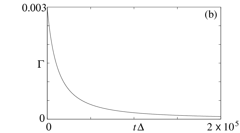

The RHS of Eq. (24) as the function of is shown in Fig. 6(a). Since the rate reaches as the parameter approaches degeneracy, we cannot conclude directly from this dependence whether the path can be traversed adiabatically or not. The adiabatic variation of the parameter calculated from Eq. (24) is shown in Fig. 6(b). Apparently we can get arbitrarily close to the level crossing in an adiabatic manner, but the question whether we can reach the point exactly in a finite time is answered in Fig. 6(c). Expressing the result in the form we can see that the function has positive second derivative, which means that decreases more slowly than exponentially. Since even at exponential decrease the degeneracy is reached at , in our case the adiabatic variation would last infinitely long as well (and thus the paths chosen for the STIRAP experiments are not really optimal for this process, even if the nonadiabatic corrections stenholm turn out to be negligibly small).
Alternative path for this process, which would not violate the adiabatic approximation at any point, could be constructed in the following way: first we switch on the pulse to some finite value while keeping . Along this line the parameters characterizing the states, and are constant, and no mixing is possible, regardless of the time of the variation. Then we could modify the parameters along the arc up to the point . Along this arc the energy difference between the states and is constant and equals . To satisfy the usual adiabatic condition [Eq. (8)] it suffices to traverse this part of the path in a time interval much longer than . However, to make sure that there will be no resonant transitions between the states and , the function needs to satisfy [according to Eq. (7b)]
| (25) |
The path is then closed by switching off the pulse , again arbitrarily fast.
V Summary
We have shown that an adiabatic process should not be understood as a process which is necessarily slow in comparison only to the energy scales in the problem. Our treatment of the adiabatic condition proves that for some paths the transitions between different energy levels can be neglected for a finite-time evolution in an infinite time scale regions. Moreover, as many of the other adiabatic phenomena, transformations within one, nondegenerate level between two points of degeneracy (corresponding to the same point in the parameter space) are geometric. The result depends only on the initial and final directions of the path, not on its details (as long as it is adiabatic). Our results, together with the theory of geometric transformations, give also the possibility of designing experiments which combine the geometric (Berry) phases, holonomic transformations (within degenerate levels), and adiabatic passage.
Acknowledgements.
The author thanks R. W. Chhajlany, R. Unanyan, and S. Stenholm for discussions and comments. This work was partly supported by the DFG-Schwerpunktprogramm “Quanten-Informationsverarbeitung.”References
- Berry (1984) M. V. Berry, Proc. R. Soc. London, Ser. A 392, 45 (1984).
- (2) J. Samuel and R. Bhandari, Phys. Rev. Lett. 60, 2339 (1988).
- (3) S. Pancharatnam, Proc. Indian Acad. Sci. A44, 247 (1956).
- (4) F. Wilczek and A. Zee, Phys. Rev. Lett. 52, 2111 (1984).
- (5) K. Bergmann, H. Theuer, and B. W. Shore, Rev. Mod. Phys. 70, 1003 (1998).
- Avron and Elgart (1999) J. E. Avron and A. Elgart, Commun. Math. Phys. 203, 445 (1999).
- Low (1989) F. E. Low, Phys. Rev. Lett 63, 2322 (1989).
- (8) T. A. Laine and S. Stenholm, Phys. Rev. A 53, 2501 (1996).
- (9) H. Pothier, P. Lafarge, C. Urbina, D. Esteve, and M.H. Devoret, Europhys. Lett. 17, 249 (1992).
- (10) J.P. Pekola, A.B. Zorin, and M.A. Paalanen, Phys. Rev. B 50, R11255 (1994).
- (11) M.W. Keller, J.M. Martinis, N.N. Zimmerman, and A.H. Steinbach, Appl. Phys. Lett. 69, 1804 (1996).