A large family of quantum weak coin-flipping protocols

Carlos Mochon Email: carlosm@theory.caltech.edu Affiliation: Institute for Quantum Information, California Institute of Technology, Pasadena, CA 91125, USA

December 25, 2005

Abstract

Each classical public-coin protocol for coin flipping is naturally associated with a quantum protocol for weak coin flipping. The quantum protocol is obtained by replacing classical randomness with quantum entanglement and by adding a cheat detection test in the last round that verifies the integrity of this entanglement. The set of such protocols defines a family which contains the protocol with bias $0.192$ previously found by the author, as well as protocols with bias as low as $1/6$ described herein. The family is analyzed by identifying a set of optimal protocols for every number of messages. In the end, tight lower bounds for the bias are obtained which prove that $1/6$ is optimal for all protocols within the family.

pacs

03.67.Hk

I Introduction

Quantum weak coin flipping is a two party quantum protocol for agreeing on a random classical bit, where Alice wants outcome zero and Bob wants outcome one. Its main constraint is that a cheating player should not be able to bias the coin in their favor by more than some parameter $\epsilon$ .

Previous work by the same author Mochon 2004a has shown that there exists a quantum weak coin-flipping protocol with bias $\epsilon=0.192$ , that is, such that neither player can win by cheating with a probability greater than $0.692$ . The protocol with bias $0.192$ was a generalization of the one by Spekkens and Rudolph Spekkens and Rudolph 2002a which achieved a bias of $1/\sqrt{2}-1/2\simeq 0.207$ . Both belong to a large family of quantum weak coin-flipping protocols that are based on a set of classical games involving public coins.

The purpose of this paper is to study this large family of protocols for quantum weak coin flipping. In particular, we will prove that the optimal protocol in this family has a bias of $1/6$ , though such a bias can only be reached in the limit of arbitrarily large messages. Because our lower bound analysis is constructive, we shall give explicit descriptions of protocols with biases that are arbitrarily close to $1/6$ .

The protocols with bias of $1/\sqrt{2}-1/2$ was originally described in Ref. Spekkens and Rudolph 2002a as part of a different family of protocols for quantum weak coin flipping, all of which involved three messages. Lower bounds for this family were obtained by Ambainis Ambainis 2002, which proved that the $\epsilon=1/\sqrt{2}-1/2$ protocol was optimal within the family. Though our family does not contain every protocol in the Spekkens and Rudolph family, it does contain its optimal protocol.

The best lower bound currently known that applies to all weak coin-flipping protocols is by Ambainis Ambainis 2001 and states that the number of messages must grow at least as $\Omega(\log\log\frac{1}{\epsilon})$ . Ambainis’ result rules out attaining an arbitrarily small bias with a fixed number of messages, thus the importance of looking at protocols with arbitrarily large number of messages. We believe that our result is the first of its kind in lower bounding the bias of a large family of protocols that includes instances with every number of messages.

Other important work related to quantum weak coin flipping includes Refs. Lo and Chau 1998; Goldenberg et al. 1999; Spekkens and Rudolph 2002b; Mochon 2004b; Rudolph and Spekkens 2004; Kerenidis and Nayak 2004 among others. Also related are the results on quantum strong coin flipping (a variant where ideally neither player should be allowed to bias the coin in either direction). The best known protocol for strong coin flipping has a bias of $1/4$ Ambainis 2001; Spekkens and Rudolph 2002b whereas Kitaev Kitaev has proven a lower bound of $1/\sqrt{2}-1/2$ for the optimal bias.

Before proceeding we shall give a working definition of quantum weak coin flipping as a quantum communication protocol where two parties (Alice and Bob) start off unentangled and then exchange a series of sequential quantum messages after which they must each output a single classical bit. Their outputs are required to satisfy the following constraints

•

If Alice and Bob both follow the protocol their outputs must always agree. Furthermore, the probability that Alice wins (i.e., both parties output zero) is given by $P_{A}$ whereas the probability that Bob wins (i.e., both parties output one) is given by $P_{B}=1-P_{A}$ .
•

If Alice is honest (i.e., follows the protocol), then independent of Bob’s actions, Alice will not output one with a probability greater than $P_{B}^{*}$ .
•

Similarly, if Bob is honest and Alice is dishonest, Bob will not output zero with a probability greater than $P_{A}^{*}$ .

The only security assumption for the above protocol is that a cheating player cannot directly affect the qubits in their opponent’s laboratory; that is, we desire protocols with information-theoretic security.

The parameters $P_{A}$ , $P_{A}^{*}$ and $P_{B}^{*}$ will be used to describe a coin-flipping protocol. Obviously, we’d like to make $P_{A}^{*}$ and $P_{B}^{*}$ as small as possible. For simplicity, the merit of a coin-flipping protocol is often quoted by specifying the bias $\epsilon=\max(P_{A}^{*},P_{B}^{*})-1/2$ .

Note that whereas the usual definition of coin flipping requires $P_{A}=P_{B}=1/2$ , we will allow in this paper any value of $P_{A}\in[0,1]$ . This will allow us to derive a set of tradeoff curves for $P_{A}^{*}$ versus $P_{B}^{*}$ .

The rest of the paper is organized as follows: Sec. II describes some of our notation concerning tree variables, and will introduce the theorem relating classical coin games to quantum protocols for weak coin flipping. The theorem, which is a generalization of the work in Ref. Mochon 2004a, is proven in Appendix A. Though the full description of the quantum protocol is only given in the appendix, a brief description is presented at the end of Sec. II.

The main new results of the paper are presented in the two subsequent sections: the proof of lower bounds for the bias in Sec. III and the description of matching protocols in Sec. IV.

We also include in Appendix B an analytic derivation of the bias $\epsilon=0.192$ of Ref. Mochon 2004a which was originally found using numerical techniques. Though the result itself has been superseded by the protocols with bias $1/6$ , we include the derivation because it uses a fairly different set of techniques that could potentially be useful elsewhere.

II Notation

Throughout this paper we shall make ample use of binary trees. All trees henceforth will be composed exclusively of binary nodes and leaves, and the leaves will all be located at the same depth.

The nodes of a tree will be labeled by binary strings so that the leftmost node at depth $k$ gets labeled by $k$ zeroes, and the rest will equal one plus the binary value of the node to their left (keeping the number of digits constant). The root node will be denoted by the letter $r$ , which will behave as the empty string so that $x=r$ implies $x0=0$ and $x1=1$ . With these conventions the left descendant of node $x$ is $x0$ and the right descendant is $x1$ . We define $|x|$ as the length of the binary string $x$ , which also corresponds to the depth of node $x$ .

In this paper we shall use calligraphic fonts, such as $\mathcal{G}$ , to denote an assignment of a number or expression to each node of a binary tree. Given an assignment $\mathcal{G}$ , the value of node $x$ will be $\mathcal{G}_{x}$ . Most of our notation is summarized by Fig. 1. Note that, though we shall always be working with trees of fixed finite depth, we shall usually leave the depth implicit.

Figure 1: A depth 3 binary tree.

We define an $n$ -Coin-Game as an assignment $\mathcal{G}$ to a depth $n$ binary tree such that $\mathcal{G}_{x}\in[0,1]$ for all $x$ and $\mathcal{G}_{x}\in\{0,1\}$ for all leaves (i.e., for all $x$ such that $|x|=n$ ). To each $n$ -Coin-Game, $\mathcal{G}$ , we can associate a classical $n$ -message public-coin coin-flipping protocol as follows: The state of the protocol at each step will be described by a node in the tree, and this information will be kept by both Alice and Bob. The game begins at the root node and proceeds downward until reaching a leaf node. If the current node $x$ is a binary node of even depth, then Alice chooses which path to follow and announces the choice to Bob. This is done probabilistically, by announcing the outcome of a public coin with bias $\mathcal{G}_{x}$ , so that Alice chooses the left path with probability $\mathcal{G}_{x}$ and the right path with probability $1-\mathcal{G}_{x}$ . The same mechanism occurs at odd binary nodes, except that Bob is responsible for choosing the direction and announcing it to Alice. The game ends when arriving at a leaf node $x$ , in which case Alice wins if $\mathcal{G}_{x}=0$ and Bob wins if $\mathcal{G}_{x}=1$ .

Note that we do not require that the coin-flip be fair when both Alice and Bob are honest. Given an $n$ -Coin-Game $\mathcal{G}$ , we can define $\mathcal{H}$ on a tree of the same depth by the equations:

\displaystyle\mathcal{H}_{x}=\begin{cases}\mathcal{G}_{x}&\text{if $|x|=n$,}\\ \mathcal{G}_{x}\mathcal{H}_{x0}+(1-\mathcal{G}_{x})\mathcal{H}_{x1}&\text{if $|x|<n$.}\end{cases}

(1)

The value of $\mathcal{H}_{x}$ indicates the conditional probability that Bob would win given that the game arrived at node $x$ , assuming both players play honestly. The value of $\mathcal{H}_{r}$ is Bob’s probability of winning for an honest game, which is clearly bounded between 0 and 1.

For each $n$ -Coin-Game $\mathcal{G}$ , we also define $\mathcal{A}$ and $\mathcal{B}$ on a tree of the same depth by the equations:

	$\displaystyle\mathcal{A}_{x}=\begin{cases}1-\mathcal{G}_{x}&\text{for $\|x\|=n$,}\\ \mathcal{G}_{x}\mathcal{A}_{x0}^{2}+(1-\mathcal{G}_{x})\mathcal{A}_{x1}^{2}&\text{$\|x\|$ even, $\|x\|<n$,}\\ \mathcal{G}_{x}\sqrt{\mathcal{A}_{x0}}+(1-\mathcal{G}_{x})\sqrt{\mathcal{A}_{x1}}&\text{$\|x\|$ odd, $\|x\|<n$,}\\ \end{cases}$
	$\displaystyle\mathcal{B}_{x}=\begin{cases}\mathcal{G}_{x}&\text{for $\|x\|=n$,}\\ \mathcal{G}_{x}\sqrt{\mathcal{B}_{x0}}+(1-\mathcal{G}_{x})\sqrt{\mathcal{B}_{x1}}&\text{$\|x\|$ even, $\|x\|<n$,}\\ \mathcal{G}_{x}\mathcal{B}_{x0}^{2}+(1-\mathcal{G}_{x})\mathcal{B}_{x1}^{2}&\text{$\|x\|$ odd, $\|x\|<n$.}\\ \end{cases}$
			(2)

The importance of these quantities is given by the following theorem:

Theorem 1.

For each $n$ -Coin-Game, $\mathcal{G}$ , there exists an $(n+1)$ -message quantum weak coin-flipping protocol such that

	$\displaystyle P_{A}P_{A}^{*}$	$\displaystyle=$	$\displaystyle\mathcal{A}_{r},$		(3)
	$\displaystyle P_{B}P_{B}^{*}$	$\displaystyle=$	$\displaystyle\mathcal{B}_{r}^{2},$		(4)

and the honest probabilities of winning are

\displaystyle P_{A}=(1-P_{B})=(1-\mathcal{H}_{r}),

(5)

where $\mathcal{A}$ , $\mathcal{B}$ and $\mathcal{H}$ are defined in terms of $\mathcal{G}$ by Eqs. (1,2).

The quantum protocol

In this section we shall give a brief approximate description of the quantum protocol, which should provide the needed intuition. The full description of the protocol is contained in Appendix A along with the proof of the above theorem. A simpler version of the protocol also appears in Ref. Mochon 2004a.

The basic idea is to take the classical public-coin protocol associated with an $n$ -Coin-Game, $\mathcal{G}$ , replace the classical randomness with quantum entanglement, and then add a cheat detection step.

Classical shared randomness can be replaced by quantum entanglement using states of the form

\displaystyle\sqrt{a}{|{0}\rangle}\otimes{|{0}\rangle}+\sqrt{1-a}{|{1}\rangle}\otimes{|{1}\rangle},

(6)

where one qubit belongs to Alice and one to Bob. The randomness can be extracted at any time by measuring both qubits in the computational basis.

In the classical protocol associated with $\mathcal{G}$ described above, Alice and Bob slowly built up a shared random string. After the first $k$ messages they shared a random $k$ -bit string, where string $x$ has probability $\mathcal{P}_{x}$ (the formal definition of $\mathcal{P}$ is given in Eq. (69)). The quantum protocol is constructed so that, after $k$ messages, Alice and Bob share the state

\displaystyle{|{\psi_{k}}\rangle}=\sum_{\begin{subarray}{c}x\cr|x|=k\end{subarray}}\sqrt{\mathcal{P}_{x}}{|{x}\rangle}\otimes{|{x}\rangle}.

(7)

In the classical protocol, the sender of the message (Alice for odd messages and Bob for even messages) has control over its content and hence the ability to cheat at that step, whereas the other player has no control over the given step. In the quantum protocol the same structure is maintained. The basic step to go from a $k$ -bit string to a $k+1$ -bit string is for the message sender to append two qubits in the zero state, then apply a controlled unitary on the two qubits with the other $k$ bits as control, and finally to send one of the qubits to the other player:

$\displaystyle{\|{\psi_{k}}\rangle}$	$\displaystyle\longrightarrow$	$\displaystyle{\|{\psi_{k}}\rangle}\otimes{\|{00}\rangle}$	(8)
	$\displaystyle\longrightarrow$	$\displaystyle\sum_{\begin{subarray}{c}x\cr\|x\|=k\end{subarray}}\sqrt{\mathcal{P}_{x}}{\|{x}\rangle}_{A}\otimes{\|{x}\rangle}_{B}$
		$\displaystyle\qquad\quad\otimes\left(\sqrt{\mathcal{G}_{x}}{\|{00}\rangle}+\sqrt{1-\mathcal{G}_{x}}{\|{11}\rangle}\right)$
	$\displaystyle\longrightarrow$	$\displaystyle\sum_{\begin{subarray}{c}x\cr\|x\|=k\end{subarray}}\sum_{i\in\{0,1\}}\sqrt{\mathcal{P}_{xi}}{\|{xi}\rangle}_{A}\otimes{\|{xi}\rangle}_{B}={\|{\psi_{k+1}}\rangle}.$

After $n$ messages, at the end of the classical protocol, Alice and Bob share an $n$ -bit string, which determines the coin outcome based on the value of the corresponding leaf of $\mathcal{G}$ . In the quantum protocol, they do the equivalent measurement, but using a two outcome POVM so that most of the entanglement is preserved after the measurement. This allows a cheat detection step to be appended to the end of the protocol as follows: the winner of the coin-flip based on the POVM must send over all of their qubits to the other player for inspection. The other player will end up with a pure state and can do a projection onto the final state and its complement. If the latter result is obtained, then cheating is detected and the losing player can declare victory, otherwise that player acknowledges defeat. In either case, the first player always declares victory.

Note that, though it is possible for both players to declare victory at the same time, this can only occur if one of them was cheating, and in such cases we always expect the cheating player to declare victory anyway.

The rest of this paper contains the analysis of the family of protocols, which will identify the protocol with bias of $1/6$ and prove that it is optimal within the family.

III Lower bounds on the bias

In this section we shall derive lower bounds for the set of $P_{A}^{*}$ and $P_{B}^{*}$ that can be achieved with quantum protocols based on $n$ -Coin-Games as defined in Theorem 1.

Definition 2.

For $n\in\mathbb{Z}^{+}$ , define the set $\Lambda_{n}\subset\mathbb{R}^{2}$ so that $(A,B)\in\Lambda_{n}$ if and only if there exists an $n$ -Coin-Game, $\mathcal{G}$ , with $A=\mathcal{A}_{r}$ and $B=\mathcal{B}_{r}$ and $\mathcal{A}$ and $\mathcal{B}$ defined in terms of $\mathcal{G}$ by Eq. (2).

For each $(A,B)\in\Lambda_{n}$ there exists an $(n+1)$ -message quantum coin-flipping protocol such that $P_{A}P_{A}^{*}=A$ and $P_{B}P_{B}^{*}=B^{2}$ . Furthermore, if $(P_{A}P_{A}^{*},\sqrt{P_{B}P_{B}^{*}})\notin\Lambda_{n}$ then there is no protocol built out of a $n$ -Coin-Game that achieves $P_{A}$ , $P_{A}^{*}$ and $P_{B}^{*}$ . However, it is not true that $(P_{A}P_{A}^{*},\sqrt{P_{B}P_{B}^{*}})\in\Lambda_{n}$ implies the existence of a protocol with those parameters. For example, $(0.3531,\sqrt{0.3531})\in\Lambda_{2}$ because there exists a $3$ -message protocol with $P_{A}\simeq 0.515$ , $P_{A}^{*}\simeq 0.686$ , $P_{B}^{*}\simeq 0.728$ , however there are no $3$ -message protocols with $P_{A}=P_{B}=1/2$ and $P_{A}^{*}=P_{B}^{*}\simeq 2*0.353=0.706$ . The optimal symmetric 3-message protocol is the one by Spekkens and Rudolph Spekkens and Rudolph 2002a with $P_{A}^{*}=P_{B}^{*}=1/\sqrt{2}=0.707$ . Though it would be preferable to study the set of achievable triplets $(\mathcal{A}_{r},\mathcal{B}_{r},\mathcal{H}_{r})$ , the sets $\Lambda_{n}$ are easier to analyze and in the limit $n\rightarrow\infty$ will provide us with interesting bounds.

We begin the study of the sets $\Lambda_{n}$ by showing that they can be obtained inductively:

Lemma 3.

The set $\Lambda_{n}$ is the convex combination of pairs of points from the set $\{(B^{2},\sqrt{A})\,|\,(A,B)\in\Lambda_{n-1}\}$ .

Proof.

Given an $n$ -Coin-Game, $\mathcal{G}$ , define the variable $\gamma\equiv\mathcal{G}_{r}\in[0,1]$ and the two $(n-1)$ -Coin-Games $\mathcal{G}^{(0)}$ and $\mathcal{G}^{(1)}$ by

\displaystyle\mathcal{G}^{(i)}_{x}=\begin{cases}1-\mathcal{G}_{ix}&\ \ \text{for $\ |x|=n-1$,}\\ \mathcal{G}_{ix}&\ \ \text{for $\ |x|<n-1$,}\end{cases}

(9)

for $i=0,1$ . There is a natural isomorphism between $\mathcal{G}$ and the triplet $\gamma,\mathcal{G}^{(0)},\mathcal{G}^{(1)}$ .

Furthermore define $\mathcal{A}^{(i)}$ and $\mathcal{B}^{(i)}$ in terms of $\mathcal{G}^{(i)}$ in the usual way. Note that $\mathcal{A}^{(i)}$ and $\mathcal{B}^{(i)}$ are not the left and right branches of $\mathcal{A}$ and $\mathcal{B}$ defined from $\mathcal{G}$ but rather $\mathcal{A}^{(i)}_{x}=\mathcal{B}_{ix}$ and $\mathcal{B}^{(i)}_{x}=\mathcal{A}_{ix}$ . Therefore

	$\displaystyle\mathcal{A}_{r}$	$\displaystyle=$	$\displaystyle\gamma\left(\mathcal{B}_{r}^{(0)}\right)^{2}+(1-\gamma)\left(\mathcal{B}_{r}^{(1)}\right)^{2},$		(10)
	$\displaystyle\mathcal{B}_{r}$	$\displaystyle=$	$\displaystyle\gamma\sqrt{\mathcal{A}_{r}^{(0)}}+(1-\gamma)\sqrt{\mathcal{A}_{r}^{(1)}}.$		(11)

∎

The set $\Lambda_{1}$ is fairly simple and corresponds to the convex combinations of the two points $(1,0)$ and $(0,1)$ , which could be thought of as comprising $\Lambda_{0}$ . Using $\Lambda_{1}$ and the above lemma we can prove two simple properties of the sets $\Lambda_{n}$ :

1.

$(0,1)\in\Lambda_{n}$ and $(1,0)\in\Lambda_{n}$ for all $n$ .
2.

$\Lambda_{n}\subset[0,1]\times[0,1]$ for all $n$ .

Both properties are clearly true for $\Lambda_{1}$ . By induction $(0,1)\in\Lambda_{n-1}$ and $(1,0)\in\Lambda_{n-1}$ implies that $(1^{2},\sqrt{0})$ and $(0^{2},\sqrt{1})$ are in $\Lambda_{n}$ . Similarly, if $(A,B)\in\Lambda_{n-1}$ implies $A\in[0,1]$ and $B\in[0,1]$ , then $(B^{2},\sqrt{A})\in[0,1]\times[0,1]$ and so are convex combinations of such points.

The first non-trivial set is $\Lambda_{2}$ which is the convex combination of the points on the curve $(t^{2},\sqrt{1-t})$ for $t\in[0,1]$ . The curve is plotted in Fig. 2. The dotted line marks the lower boundary of its convex hull which can be achieved using convex combinations of two points (the rest of the lower boundary of the convex hull is simply the curve itself).

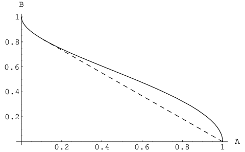
Refer to caption — Figure 2: The curve $(t^{2},\sqrt{1-t})$ for $t\in[0,1]$ . The convex hull of the curve is the region $\Lambda_{2}$ , with the dashed line serving as lower boundary.

Rather than keeping track of the sets $\Lambda_{n}$ , it will be simpler to study exclusively their lower boundary, which will be curves connecting the points $(1,0)$ and $(0,1)$ . All the optimal protocols will live on these curves, and all points below the curves will be unattainable. To formalize the notion of lower boundary we associate to every function $f(z):[0,1]\rightarrow[0,1]$ the following sets:

$\displaystyle f^{+}$	$\displaystyle=$	$\displaystyle\{(z,w)\,\|\,z\in[0,1],f(z)<w\leq 1\},$	(12)
$\displaystyle f^{=}$	$\displaystyle=$	$\displaystyle\{(z,w)\,\|\,z\in[0,1],f(z)=w\},$	(13)
$\displaystyle f^{-}$	$\displaystyle=$	$\displaystyle\{(z,w)\,\|\,z\in[0,1],f(z)>w\geq 0\}.$	(14)

Returning to the case of $\Lambda_{2}$ and Fig. 2, we see that the lower boundary follows the original curve $\sqrt{1-\sqrt{z}}$ between $(1,0)$ and some point which we shall call $(\alpha_{2},\beta_{2})$ . It then turns into a straight line connecting the point $(\alpha_{2},\beta_{2})$ to the point $(0,1)$ . The point $(\alpha_{2},\beta_{2})$ can be found by calculating the slope of the line connecting each point to $(0,1)$ and choosing the point that achieves the maximum.

In fact, all of the lower boundaries will have this form. Define for $n>1$

\displaystyle f_{n}(z)=\begin{cases}\sqrt{1-\left(\frac{1-\beta_{n}^{2}}{\sqrt{\alpha_{n}}}\right)\sqrt{z}}&\text{for $z\in[0,\alpha_{n}]$,}\\ \frac{\beta_{n}}{1-\alpha_{n}}(1-z)&\text{for $z\in[\alpha_{n},1]$,}\end{cases}

(15)

where

\displaystyle\alpha_{n}=\frac{n-1}{3(n+1)},\quad\quad\beta_{n}=\sqrt{\frac{n+2}{3n}}.

(16)

For the case $n=1$ we define $f_{1}(z)=1-z$ , which is the limit of $f_{n}$ as $n\rightarrow 1$ . Because $\alpha_{n}\in(0,1)$ and $\beta_{n}\in(0,1)$ for all $n>1$ , the functions satisfy $f_{n}(z)\in[0,1]$ for all $z\in[0,1]$ . These functions are also the lower boundaries of convex regions:

Lemma 4.

For all $n\geq 1$ , the function $f_{n}$ is strictly decreasing, and the region $f_{n}^{=}\cup f_{n}^{+}$ is convex.

Proof.

The case of $n=1$ is trivial. For $n>1$ we have

\displaystyle f_{n}^{\prime}(z)=\begin{cases}-\frac{1-\beta_{n}^{2}}{4\sqrt{\alpha_{n}}\sqrt{z}f_{n}(z)}&\text{for $z\in[0,\alpha_{n}]$,}\\ -\frac{\beta_{n}}{1-\alpha_{n}}&\text{for $z\in[\alpha_{n},1]$,}\end{cases}

(17)

which is well defined and negative on $(0,1]$ . For $z$ near zero, $f(z)\simeq 1-(1-\beta_{n}^{2})/(2\sqrt{\alpha_{n}})\sqrt{z}$ , therefore $f(z)$ is also strictly decreasing at $z=0$ .

The derivative is also continuous on $(0,1]$ because at $z=\alpha_{n}$ we have

\displaystyle\frac{\beta_{n}}{1-\alpha_{n}}=\frac{\sqrt{3}(n+1)}{2\sqrt{n(n+2)}}=\frac{1-\beta_{n}^{2}}{4\alpha_{n}\beta_{n}}.

(18)

Furthermore, in the region $(0,\alpha_{n})$ , the second derivative is

	$\displaystyle f_{n}^{\prime\prime}(z)$	$\displaystyle=$	$\displaystyle f^{\prime}_{n}(z)\left[-\frac{1}{2z}-\frac{f_{n}^{\prime}(z)}{f_{n}(z)}\right]$		(19)
		$\displaystyle=$	$\displaystyle\frac{-f_{n}^{\prime}(z)}{4z\sqrt{\alpha_{n}}f_{n}^{2}(z)}\left[2\sqrt{\alpha_{n}}-3(1-\beta_{n}^{2})\sqrt{z}\right]>0$		(19)

where the inequality holds because $3(1-\beta_{n}^{2})<2$ . Therefore $f^{\prime}_{n}(z)$ is monotonically increasing on $(0,1]$ , and the region above $f_{n}(z)$ in this interval is convex. The point $(0,1)$ can be included because the closure of a convex set is convex. ∎

We are now ready to prove the main lemma of this section.

Lemma 5.

For all $n\in\mathbb{Z}^{+}$ , $\Lambda_{n}\subset f_{n}^{=}\cup f_{n}^{+}$ and $f_{n}^{=}\subset\Lambda_{n}$ .

Proof.

The statement is clearly true for $n=1$ since $\Lambda_{1}=f_{1}^{=}$ . We will prove the rest of the cases inductively. Assume the theorem holds for $\Lambda_{n}$ , which implies that $(z,f_{n}(z))\in\Lambda_{n}$ for all $z$ . By Lemma 3 we have that $(f^{2}_{n}(z),\sqrt{z})\in\Lambda_{n+1}$ for all $z\in[0,1]$ and so are convex combinations of pairs of such points. The curve parametrized by $(f^{2}_{n}(z),\sqrt{z})$ can also be described by the points $(w,g_{n}(w))$ for

\displaystyle g_{n}(w)=\begin{cases}\sqrt{1-\left(\frac{1-\alpha_{n}}{\beta_{n}}\right)\sqrt{w}}&\text{for $w\in[0,\beta_{n}^{2}]$,}\\ \frac{\sqrt{\alpha_{n}}}{1-\beta_{n}^{2}}(1-w)&\text{for $w\in[\beta_{n}^{2},1]$.}\end{cases}

(20)

Note how under the map $(x,y)\rightarrow(y^{2},\sqrt{x})$ the straight line turns into a curve, and the curve turns into a straight line. Furthermore, because of the exchange of $x$ and $y$ , the straight line ends up on the right-hand side.

The pattern of points $\alpha_{n}$ and $\beta_{n}$ , in addition to guaranteeing that the region above $f_{n}(z)$ is convex, also satisfies the recursion relation

\displaystyle\frac{1-\alpha_{n}}{\beta_{n}}=\frac{2\sqrt{n(n+2)}}{\sqrt{3}(n+1)}=\frac{1-\beta_{n+1}^{2}}{\sqrt{\alpha_{n+1}}}

(21)

and therefore $g_{n}(z)=f_{n+1}(z)$ in the region $[0,\alpha_{n+1}]$ (since $\alpha_{n+1}\leq 1/3\leq\beta_{n}^{2}$ ). Pictorially, the curve $g_{n}^{=}$ is like the curve $f_{n+1}^{=}$ , except that the straight line intersects the curve somewhat to the right, and hence the region above $g_{n}^{=}$ is not convex. Its convex hull will give us the region above the curve $f_{n+1}^{=}$ .

Thus far we have shown $g_{n}^{=}\subset\Lambda_{n+1}$ , as are convex combinations of pairs of points on the curve $g_{n}^{=}$ . Because $g_{n}^{=}=f_{n+1}^{=}$ in the region $[0,\alpha_{n+1}]$ we know that this segment of the curve is in $\Lambda_{n+1}$ . The rest of the curve $f_{n+1}^{=}$ is simply the convex combination of the points $(\alpha_{n+1},\beta_{n+1})$ and $(1,0)$ both of which are in $g_{n}^{=}$ . We have therefore proven the second part of the lemma: $f_{n+1}^{=}\subset\Lambda_{n+1}$ .

We now intend to prove that $g_{n}(z)\geq f_{n+1}(z)$ for all $z\in[0,1]$ . The statement is clearly true in the region $[0,\alpha_{n+1}]$ where both are equal. In the region $[\beta_{n}^{2},1]$ it is also true because both functions are straight lines ending in $(1,0)$ , and the starting point of the lines are $g_{n}(\beta_{n}^{2})=\sqrt{\alpha_{n}}$ and $f_{n+1}(\beta_{n}^{2})=\beta_{n+1}(1-\beta_{n}^{2})/(1-\alpha_{n+1})$ . The inequality $f_{n+1}(\beta_{n}^{2})\geq g_{n}(\beta_{n}^{2})$ can be proven by checking that $[f_{n+1}(\beta_{n}^{2})/g_{n}(\beta_{n}^{2})]^{2}-1=-4/[n^{2}(n+3)]\leq 0$ for $n\geq 1$ . Finally, in the region $[\alpha_{n+1},\beta_{n}^{2}]$ the functions $f_{n+1}(z)$ and $g_{n}(z)$ start off at the same point, with the same derivative, but $f_{n+1}^{\prime\prime}(z)=0$ in this region whereas $g_{n}^{\prime\prime}(z)$ initially is positive, and has only one zero in the region, which can be checked as in Eq. (19). If the curve $g_{n}$ were to cross the curve $f_{n+1}$ at any point in this region, then it would have to end below it. However, we already argued that $g_{n}(\beta_{n}^{2})\geq f_{n+1}(\beta_{n}^{2})$ and therefore the curve $g_{n}^{=}$ must lie above the curve $f_{n+1}^{=}$ in the middle region as well.

So far we have shown that $(g_{n}^{=}\cup g_{n}^{+})\subset(f_{n+1}^{=}\cup f_{n+1}^{+})$ . By the induction assumption, $\Lambda_{n}\subset f_{n}^{=}\cup f_{n}^{+}$ . Under the map $(x,y)\rightarrow(y^{2},\sqrt{x})$ , the region $f_{n}^{=}\cup f_{n}^{+}$ maps into the region to the right of the curve $g_{n}^{=}$ , which also equals the region $g_{n}^{=}\cup g_{n}^{+}$ because $g_{n}(z)$ is strictly decreasing, $g_{n}(1)=0$ , and $g_{n}(0)=1$ . Finally, using Lemma 3 we know that $\Lambda_{n+1}$ is contained in the convex combination of points in $g_{n}^{=}\cup g_{n}^{+}$ . Because $(g_{n}^{=}\cup g_{n}^{+})\subset(f_{n+1}^{=}\cup f_{n+1}^{+})$ , and $f_{n+1}^{=}\cup f_{n+1}^{+}$ is convex, we have $\Lambda_{n+1}\subset f_{n+1}^{=}\cup f_{n+1}^{+}$ . ∎

Combining the previous lemma with the definition of the sets $\Lambda_{n}$ , we have proven the following theorem:

Theorem 6.

Every $(n+1)$ -message quantum weak coin-flipping protocol based on an $n$ -Coin-Game satisfies

\displaystyle P_{B}P_{B}^{*}\geq f_{n}^{2}(P_{A}P_{A}^{*}).

(22)

Additionally, we have the following corollary for the limit of $n\rightarrow\infty$ :

Corollary 7.

All quantum weak coin-flipping protocols based on an $n$ -Coin-Game (for any $n\in\mathbb{Z}^{+}$ ) satisfy

	$\displaystyle P_{A}P_{A}^{}\leq\frac{1}{3}\quad\Longrightarrow\quad P_{B}P_{B}^{}\geq 1-2\sqrt{\frac{P_{A}P_{A}^{*}}{3}}\geq\frac{1}{3}$		(23)
	$\displaystyle P_{B}P_{B}^{}\leq\frac{1}{3}\quad\Longrightarrow\quad P_{A}P_{A}^{}\geq 1-2\sqrt{\frac{P_{B}P_{B}^{*}}{3}}\geq\frac{1}{3}$		(24)

In particular,

\displaystyle\max\left(P_{A}P_{A}^{*},P_{B}P_{B}^{*}\right)\geq\frac{1}{3},

(25)

and

\displaystyle\max(P_{A}^{*},P_{B}^{*})\geq\frac{2}{3}\ \ \ \ \text{for $\ P_{A}=P_{B}=\frac{1}{2}$}.

(26)

Proof.

The above results use the limit:

\displaystyle f_{\infty}(z)=\begin{cases}\sqrt{1-\frac{2}{\sqrt{3}}\sqrt{z}}&\text{for $z\in[0,\frac{1}{3}]$,}\\ \frac{\sqrt{3}}{2}(1-z)&\text{for $z\in[\frac{1}{3},1]$,}\end{cases}

(27)

which has the symmetry $b=f_{\infty}^{2}(a)\Rightarrow a=f_{\infty}^{2}(b)$ . ∎

IV Optimal Protocols

In this section we will describe protocols that match the lower bounds derived in the previous section. In a sense, most of the work has already been done since the proof of the previous section was constructive. What remains undone is to explicitly construct the $n$ -Coin-Games and to calculate from them $P_{A}$ , $P_{A}^{*}$ and $P_{B}^{*}$ (rather than only their products).

From the discussion of the previous section we can see that the interesting $(n+1)$ -Coin-Games live on the curve $f_{n+1}^{=}$ . The points on the rounded part of the curve (the left segment) involve no convex combinations of points from $n$ -Coin-Games and therefore are not new (i.e., they are protocols that can be described by a single $n$ -Coin-Game with Alice’s and Bob’s role reversed). The interesting points at level $n+1$ lie on the straight segment and are the combination of the points $(\alpha_{n+1},\beta_{n+1})$ and $(1,0)$ . To understand this segment we need to describe the $n$ -Coin-Games that produce points $(\beta_{n+1}^{2},\sqrt{\alpha_{n+1}})$ and $(0,1)$ . The second point corresponds to a tree that is fairly simple: it has the value $1$ at every leaf and the rest of the nodes are irrelevant. The $n$ -Coin-Games for $(\beta_{n+1}^{2},\sqrt{\alpha_{n+1}})$ is what we shall describe next.

Lemma 8.

For each $n\in\mathbb{Z}^{+}$ there is an $n$ -Coin-Game, $\mathcal{G}^{(n)}$ , such that

$\displaystyle\mathcal{A}^{(n)}_{r}$	$\displaystyle=$	$\displaystyle\beta_{n+1}^{2}=\frac{n+3}{3(n+1)},$	(28)
$\displaystyle\mathcal{B}^{(n)}_{r}$	$\displaystyle=$	$\displaystyle\sqrt{\alpha_{n+1}}=\sqrt{\frac{n}{3(n+2)}},$	(29)
$\displaystyle\mathcal{H}^{(n)}_{r}$	$\displaystyle=$	$\displaystyle\begin{cases}\frac{n}{2(n+1)}&\text{$n$ even},\\ \frac{n+1}{2(n+2)}&\text{$n$ odd},\end{cases}$	(30)

with $\mathcal{A}^{(n)}$ , $\mathcal{B}^{(n)}$ and $\mathcal{H}^{(n)}$ defined in terms of $\mathcal{G}^{(n)}$ by Eqs. (1,2). In particular, the associated quantum weak coin-flipping protocols have:

$\displaystyle P_{A}(n)=$	$\displaystyle 1-\mathcal{H}^{(n)}_{r}$	$\displaystyle=\begin{cases}\frac{n+2}{2(n+1)}&\text{$n$ even},\\ \frac{n+3}{2(n+2)}&\text{$n$ odd},\end{cases}$	(31)
$\displaystyle P_{A}^{*}(n)=$	$\displaystyle\frac{\mathcal{A}^{(n)}_{r}}{1-\mathcal{H}^{(n)}_{r}}$	$\displaystyle=\begin{cases}\frac{2(n+3)}{3(n+2)}&\text{$n$ even},\\ \frac{2(n+2)}{3(n+1)}&\text{$n$ odd},\end{cases}$	(32)
$\displaystyle P_{B}^{*}(n)=$	$\displaystyle\frac{\left(\mathcal{B}^{(n)}_{r}\right)^{2}}{\mathcal{H}^{(n)}_{r}}$	$\displaystyle=\begin{cases}\frac{2(n+1)}{3(n+2)}&\text{$n$ even},\\ \frac{2n}{3(n+1)}&\text{$n$ odd}.\end{cases}$	(33)

Proof.

Define the parameters

\displaystyle\gamma_{n}=\frac{n}{n+2},

(34)

which are the weights needed for the convex combinations. And let

\displaystyle\mathcal{G}^{(1)}_{r}=\gamma_{1},\ \ \ \ \mathcal{G}^{(1)}_{0}=1,\ \ \ \ \mathcal{G}^{(1)}_{1}=0,

(35)

which leads to $\mathcal{A}_{r}^{(1)}=2/3$ and $\mathcal{B}_{r}^{(1)}=\mathcal{H}_{r}^{(1)}=1/3$ . The rest of the Coin-Games are defined inductively:

$\displaystyle\mathcal{G}^{(n)}_{r}$	$\displaystyle=$	$\displaystyle\gamma_{n},$	(36)
$\displaystyle\mathcal{G}^{(n)}_{0x}$	$\displaystyle=$	$\displaystyle\begin{cases}1-\mathcal{G}^{(n-1)}_{x}&\ \text{for $\ \|x\|=n-1$},\\ \mathcal{G}^{(n-1)}_{x}&\ \text{for $\ \|x\|<n-1$},\\ \end{cases}$	(37)
$\displaystyle\mathcal{G}^{(n)}_{1x}$	$\displaystyle=$	$\displaystyle\begin{cases}0&\ \ \ \ \ \ \text{for $\ \|x\|=n-1$},\\ \mathcal{G}^{(n-1)}_{x}&\ \ \ \ \ \ \text{for $\ \|x\|<n-1$}.\\ \end{cases}$	(38)

The values of $\mathcal{G}^{(n)}_{1x}$ for $|x|<n-1$ are actually irrelevant but were chosen so that $\mathcal{G}^{(n)}_{x}=\gamma_{n-|x|}$ whenever $|x|<n-1$ , and therefore these protocols fit into the subfamily studied in Ref. Mochon 2004a.

The reason for inverting the value of the leaves relates to our insistence that Alice always send the first message, which implies that the sender of the last message alternates as $n$ is increased and correspondingly the assignments of winning and losing for the coin outcome need to be flipped.

In fact, the pattern of the leaves is fairly simple. It is chosen so that it depends on the parity of the location (from left to right) of the first 1 symbol in the string $x$ . In the quantum protocol this translates into the first sender of a 1 qubit being the winner of the coin-flip (assuming they pass the cheat detection phase).

In fact, the trees $\mathcal{G}^{(n)}$ would best be described by truncated trees of the form of Fig. 3. However, we shall continue using trees with all leaves at the same depth in order to be consistent with the previous section.

Figure 3: A truncated tree equivalent to

\mathcal{G}^{(4)}

Returning to the proof of the lemma, it is easy to see that $\mathcal{A}_{1x}^{(n)}=1$ and $\mathcal{B}_{1x}^{(n)}=\mathcal{H}_{1x}^{(n)}=0$ for all strings $x$ . The left side of the tree satisfies $\mathcal{A}_{0x}^{(n)}=\mathcal{B}_{x}^{(n-1)}$ , $\mathcal{B}_{0x}^{(n)}=\mathcal{A}_{x}^{(n-1)}$ and $\mathcal{H}_{0x}^{(n)}=1-\mathcal{H}_{x}^{(n-1)}$ for all strings $x$ . Therefore the root nodes are

$\displaystyle\mathcal{A}_{r}^{(n)}=$	$\displaystyle\gamma_{n}\left(\mathcal{B}_{r}^{(n-1)}\right)^{2}$	$\displaystyle+(1-\gamma_{n})\ 1,$	(39)
$\displaystyle\mathcal{B}_{r}^{(n)}=$	$\displaystyle\gamma_{n}\sqrt{\mathcal{A}_{r}^{(n-1)}}$	$\displaystyle+(1-\gamma_{n})\ 0,$	(40)
$\displaystyle\mathcal{H}_{r}^{(n)}=$	$\displaystyle\gamma_{n}\left(1-\mathcal{H}_{r}^{(n-1)}\right)$	$\displaystyle+(1-\gamma_{n})\ 0.$	(41)

It is then straightforward to plug in the expressions as functions of $n$ for all the above parameters and check that Eqs. (28–30) are always satisfied. ∎

Interestingly, the sequence of protocols is such that $P_{A}$ and $P_{B}$ do not change when $n$ increases from an odd integer to an even one, whereas $P_{A}^{*}$ and $P_{B}^{*}$ do not change when $n$ increases from an even integer to an odd one. We offer no intuition for this property. Note, however, that for a given $n$ , the associated protocol corresponds to a single point on the surface of optimal protocols in the $3$ -dimensional space of triplets $(P_{A},P_{A}^{*},P_{B}^{*})$ that can be achieved with $n+1$ quantum messages.

For large $n$ , the sequence of protocols converges to $P_{A}=P_{B}=1/2$ and $P_{A}^{*}=P_{B}^{*}=2/3$ , yielding a protocol with bias of $1/6$ . It would also be desirable to show the existence of a sequence of protocols that converges to the same point but such that $P_{A}=P_{B}=1/2$ for every protocol in the sequence. This can be easily accomplished by choosing, for each $n$ , the point along the curve $f_{n}^{=}$ that has $\mathcal{H}_{r}=1/2$ . In the Coin-Game language we need to modify the top coin $\mathcal{G}_{r}$ , and we therefore introduce a new sequence of Coin-Games ${\mathcal{G}^{\prime}}^{(n)}$ defined as

\displaystyle{\mathcal{G}^{\prime}_{x}}^{(n)}=\begin{cases}1/\left(2-2\mathcal{H}_{r}^{(n-1)}\right)&x=r,\\ \mathcal{G}^{(n)}_{x}&\text{otherwise.}\end{cases}

(42)

For simplicity, we will concentrate on the case when $n$ is even so that:

$\displaystyle{\mathcal{A}^{\prime}_{r}}^{(n)}$	$\displaystyle=$	$\displaystyle\frac{n+1}{n+2}\left(\mathcal{B}_{r}^{(n-1)}\right)^{2}+\frac{1}{n+2},$	(43)
$\displaystyle{\mathcal{B}^{\prime}_{r}}^{(n)}$	$\displaystyle=$	$\displaystyle\frac{n+1}{n+2}\sqrt{\mathcal{A}_{r}^{(n-1)}},$	(44)
$\displaystyle{\mathcal{H}^{\prime}_{r}}^{(n)}$	$\displaystyle=$	$\displaystyle\frac{n+1}{n+2}(1-\mathcal{H}_{r}^{(n-1)})=\frac{1}{2}$	(45)

and the associated probabilities of winning by cheating are

	$\displaystyle P_{A}^{*}(n)^{\prime}=$	$\displaystyle 2{\mathcal{A}^{\prime}_{r}}^{(n)}$	$\displaystyle=\frac{2}{3},$		(46)
	$\displaystyle P_{B}^{*}(n)^{\prime}=$	$\displaystyle 2\left({\mathcal{B}^{\prime}_{r}}^{(n)}\right)^{2}$	$\displaystyle=\frac{2}{3}\,\frac{(n+1)^{2}}{n(n+2)}.$		(47)

That is, we have identified a nice sequence of quantum protocols with $n+1$ messages (for $n$ even) where $P_{A}=P_{B}=1/2$ and $P_{A}^{*}=2/3$ are all fixed and $P_{B}^{*}$ decreases from $3/4$ to $2/3$ . Of course, the case $n=2$ belongs to the family studied by Spekkens and Rudolph Spekkens and Rudolph 2002a and satisfies $P_{A}^{*}P_{B}^{*}=1/2$ .

As discussed in the introduction to the previous section, the above protocols are optimal in the following sense: to decrease one of $P_{A}^{*}$ or $P_{B}^{*}$ while keeping the number of messages fixed, we would have to increase the other parameter. However, the protocols are not optimal in the sense that they minimize the bias $\epsilon=\max(P_{A}^{*},P_{B}^{*})-1/2$ for a fixed number of messages. Only in the limit of infinite messages is the bias of the above protocols optimal.

Thus far, we have identified the point $(1/3,\sqrt{1/3})\in f_{\infty}^{=}$ as a protocol with $P_{A}=1/2$ and $P_{A}^{*}=P_{B}^{*}=2/3$ . The other points on the curve $f_{\infty}^{=}$ can be found using the same trick of modifying the top coin $\mathcal{G}_{r}$ . That is, let ${\mathcal{G}^{\prime}}^{(n)}$ be as above but with ${\mathcal{G}^{\prime}_{r}}^{(n)}=t$ , where $t\in[0,1]$ is a parameter we can choose freely. In the limit of $n\rightarrow\infty$ we find:

$\displaystyle{\mathcal{A}_{r}^{\prime}}^{(\infty)}(t)$	$\displaystyle=$	$\displaystyle t\,\frac{1}{3}+(1-t),$	(48)
$\displaystyle{\mathcal{B}_{r}^{\prime}}^{(\infty)}(t)$	$\displaystyle=$	$\displaystyle t\,\sqrt{\frac{1}{3}},$	(49)
$\displaystyle{\mathcal{H}_{r}^{\prime}}^{(\infty)}(t)$	$\displaystyle=$	$\displaystyle t\,\frac{1}{2}.$	(50)

The associated quantum weak coin-flipping parameters are

$\displaystyle P_{A}(t)$	$\displaystyle=$	$\displaystyle 1-\frac{t}{2},$	(51)
$\displaystyle P_{A}^{*}(t)$	$\displaystyle=$	$\displaystyle\frac{2}{3}\,\frac{3-2t}{2-t},$	(52)
$\displaystyle P_{B}^{*}(t)$	$\displaystyle=$	$\displaystyle\frac{2}{3}\,t.$	(53)

These protocols correspond to the right half of the curve $f_{\infty}^{=}$ (i.e., the points $(z,f_{\infty}(z))$ for $z\in[1/3,1]$ ). The other half of the curve can be obtained by symmetry between Alice and Bob. In the Coin-Game formalism this symmetry arises by creating a new $(n+1)$ -Coin-Game, $\mathcal{G}^{\prime}$ , out of given $n$ -Coin-Game, $\mathcal{G}$ , by the rules $\mathcal{G}^{\prime}_{r}=1$ , $\mathcal{G}^{\prime}_{0x}=\mathcal{G}^{\prime}_{1x}=\mathcal{G}_{x}$ for $|x|<n$ and $\mathcal{G}^{\prime}_{0x}=\mathcal{G}^{\prime}_{1x}=1-\mathcal{G}_{x}$ for $|x|=n$ . In the language of protocols, we are forcing Alice’s first message to have no content, which is equivalent to allowing Bob to begin the game.

The results can be best summarized by eliminating the variable $t$ from Eqs. (51–53), which proves this section’s main theorem:

Theorem 9.

There exist quantum weak coin-flipping protocols that asymptotically approach the curve

\displaystyle P_{A}^{*}+P_{B}^{*}-\frac{3}{4}P_{A}^{*}P_{B}^{*}=1

(54)

in the limit of large number of messages. The corresponding probabilities of winning when the game is played honestly are

	$\displaystyle P_{A}$	$\displaystyle=$	$\displaystyle\frac{3}{4}\,P_{A}^{}\ \ \ \ \text{when $P_{A}^{}\leq P_{B}^{*}$},$		(55)
	$\displaystyle P_{B}$	$\displaystyle=$	$\displaystyle\frac{3}{4}\,P_{B}^{}\ \ \ \ \text{when $P_{A}^{}\geq P_{B}^{*}$}.$		(56)

Implementing the optimal protocols

Surprisingly, the optimal protocols identified above are significantly easier to describe and implement than a generic protocol associated with a random $n$ -Coin-Game. Here we shall present a brief description of the simplified protocol associated with the Coin-Games from Eqs. (42–47).

We begin by fixing a security parameter $n$ , which will lead to an $n+2$ message quantum protocol. For simplicity we assume that $n$ is even.

The first $n$ messages of the quantum protocol each involve one player preparing a two qubit entangled state and sending one of the two qubits to the other player. The two qubit states can be written as

\displaystyle\sqrt{a_{i}}{|{00}\rangle}+\sqrt{1-a_{i}}{|{11}\rangle}

(57)

for $i=1,\dots,n$ , where

\displaystyle a_{i}=\begin{cases}\frac{n+1}{n+2}&i=1,\cr\frac{n-i+1}{n-i+3}&i\neq 1.\end{cases}

(58)

As usual Alice is in charge of sending the odd messages (and hence preparing the odd numbered states) whereas Bob sends the even numbered messages.

At the end of the above procedure Alice and Bob should each have $n$ qubits, which can be expressed in a basis of $n$ -bit strings with the most significant bit corresponding to the first qubit sent or received. They now each perform a two-outcome measurement which can be described as follows: let $S$ be the set of all $n$ -bit strings such that the first occurrence of the digit one, when the bits are examined from left to right, appears at an even location, again counting from left to right (i.e., for $n=4$ we have $S=\{0001,0100,0101,0110,0111\}$ ). The two outcome measurement is given by the POVM elements

\displaystyle E_{0}=I-E_{1},\qquad E_{1}=\sum_{x\in S}{|{x}\rangle}{\langle{x}|}.

(59)

As usual Alice wins on outcome zero and Bob wins on outcome one. Note that, in essence, the first person to send a qubit in the “one” state is the winner at this stage. However, the following cheat detection step will be powerful enough to dissuade against the obvious cheating strategy.

Before outputting the final answer the party who won sends all their qubits over to the losing party who then does an extra cheat-detecting two-outcome measurement to verify that the $2n$ qubit state now in their possession is the correct one (i.e., they project onto the state and its complement). Unfortunately, this final step is likely to be very fairly difficult with current technology for any $n>2$ .

In the end, the resulting protocol goes to a bias of $1/6$ as $n$ is taken to infinity. For $n=4$ Bob’s probability of winning by cheating is $P_{B}^{*}=0.694$ whereas for $n=6$ we get $P_{B}^{*}=0.681$ . Furthermore, Alice’s cheating is always restricted at $P_{A}^{*}=2/3$ . Protocols with more symmetry between Alice and Bob can also be described as above by changing the coefficients $\{a_{i}\}$ .

V Conclusions

We have identified a large family of quantum protocols for weak coin flipping, that are based on classical public-coin games. The family contains protocols approaching the curve $P_{A}^{*}+P_{B}^{*}-\frac{3}{4}P_{A}^{*}P_{B}^{*}=1$ , which can be reached asymptotically in the limit of large number of messages. The most important of these protocols is symmetric between Alice and Bob and achieves $P_{A}=P_{B}=1/2$ and $P_{A}^{*}=P_{B}^{*}=2/3$ , that is, it has a bias of $1/6$ .

Furthermore, we have proven lower bounds for the bias achievable by protocols in this family. In particular, $\max(P_{A}^{*},P_{B}^{*})\geq 2/3$ or equivalently $\epsilon\geq 1/6$ . These lower bounds show that the protocols found above are optimal within their family.

Our lower bounds also establish a strict hierarchy among coin-flipping protocols in our family with different number of messages. Admittedly, the hierarchy is of little practical interest since a small number of messages suffices in all cases to construct protocols that are reasonably close to optimal.

Though the question of optimal bias for a general quantum weak coin-flipping protocol remains open, we speculate that it might be possible to show that every protocol is equivalent to one contained in the family analyzed in this paper. Future work will be needed to verify this conjecture.

Acknowledgements.

The author would like to thank Graeme Smith for his help in proofreading this manuscript. This work was supported in part by the National Science Foundation under grant number EIA-0086038 and by the Department of Energy under grant number DE-FG03-92-ER40701.

Appendix A The Protocol

The purpose of this appendix is to describe the $(n+1)$ -message quantum weak coin-flipping protocol associated to each $n$ -Coin-Game. For each protocol we shall also derive matching upper and lower bounds on the amount that each party can cheat and thereby prove Theorem 1.

All the general ideas needed in this section have appeared previously in Ref. Mochon 2004a, though in a somewhat different notation. The new elements of this appendix are:

1.

Ref. Mochon 2004a was restricted to $n$ -Coin-Games where all the binary nodes at the same depth had the same value (i.e, $\mathcal{G}_{x}=\mathcal{G}_{x^{\prime}}$ if $|x|=|x^{\prime}|<n$ ). These variables were given the name $a_{i}$ so that $\mathcal{G}_{x}=a_{|x|+1}$ . In this section we lift the restriction and consider general $n$ -Coin-Games.
2.

An upper bound on $P_{A}^{*}$ and $P_{B}^{*}$ was derived in Ref. Mochon 2004a but was not proven optimal. In this section we shall derive a matching lower bound.

Because most of the ideas here have been published elsewhere, we shall simply prove the necessary facts in this section without providing the intuition or motivation behind the constructions. For a more pedagogical approach we refer the reader to Ref. Mochon 2004a.

We begin by fixing an $n$ -Coin-Game $\mathcal{G}$ , which will be used throughout this section. We also fix $\mathcal{H}$ , $\mathcal{A}$ and $\mathcal{B}$ as given by Eqs. (1,2). Because optimal protocols with $\mathcal{H}_{r}=0$ and $\mathcal{H}_{r}=1$ are easy to construct even classically, for what follows we shall assume that $0<\mathcal{H}_{r}<1$ .

To describe the quantum protocol associated with $\mathcal{G}$ we employ the standard quantum communication model involving the Hilbert space decomposition $H_{A}\otimes H_{M}\otimes H_{B}$ , where $H_{A}$ is Alice’s private space, $H_{B}$ is Bob’s private space, and $H_{M}$ is the space used for passing messages. We further subdivide these spaces as follows:

$\displaystyle H_{A}$	$\displaystyle=$	$\displaystyle H_{a}\otimes H_{a^{\prime}}\otimes H_{ac},$	(60)
$\displaystyle H_{B}$	$\displaystyle=$	$\displaystyle H_{b}\otimes H_{b^{\prime}}\otimes H_{bc},$	(61)
$\displaystyle H_{M}$	$\displaystyle=$	$\displaystyle H_{m}\otimes H_{mn}.$	(62)

The spaces $H_{a}$ and $H_{b}$ each consists of $n$ qubits and will be used to store a binary string $x$ corresponding to a node in $\mathcal{G}$ . The individual qubits comprising each space will be referred to as $a_{1}$ through $a_{n}$ and $b_{1}$ though $b_{n}$ respectively. The one-qubit space $H_{m}$ will be the primary means of communication between Alice and Bob, and will be referred to as qubit $m$ .

The rest of the spaces will only be used in the last pair of messages. The spaces $H_{a^{\prime}}$ , $H_{b^{\prime}}$ and $H_{mn}$ each involve $n$ qubits whereas $H_{ac}$ and $H_{bc}$ each contain one qubit.

Before describing the protocol we need to define a set of unitaries on $H_{A}\otimes H_{M}$ . We begin with the controlled rotations $R_{A,k}$ defined for $k=1,\dots,n$ by

\displaystyle R_{A,k}=\sum_{\begin{subarray}{c}x\cr|x|=k-1\end{subarray}}{|{x}\rangle}{\langle{x}|}_{a_{1},\dots,a_{k-1}}\otimes U(\mathcal{G}_{x})_{a_{k},m},

(63)

where

\displaystyle U(z)=\begin{pmatrix}\sqrt{z}&0&0&-\sqrt{1-z}\cr 0&\sqrt{z}&-\sqrt{1-z}&0\cr 0&\sqrt{1-z}&\sqrt{z}&0\cr\sqrt{1-z}&0&0&\sqrt{z}\end{pmatrix}.

(64)

The subscripts on the operators and matrices indicate what qubits they act on, and $R_{A,k}$ acts trivially on all qubits of $H_{A}\otimes H_{M}$ not explicitly mentioned. For the case $k=1$ the operator is not a controlled rotation but rather a regular rotation using parameter $\mathcal{G}_{r}$ .

We shall also need the controlled rotation

R_{A,E}=\sum_{\begin{subarray}{c}x\cr|x|=n\end{subarray}}{|{x}\rangle}{\langle{x}|}_{a_{1},\dots,a_{n}}\otimes\begin{pmatrix}1-\mathcal{G}_{x}&-\mathcal{G}_{x}\cr\mathcal{G}_{x}&1-\mathcal{G}_{x}\end{pmatrix}_{ac},\quad

(65)

which is unitary because $\mathcal{G}_{x}\in\{0,1\}$ for $|x|=n$ . The gate is simply a controlled-X applied to the qubit in space $H_{ac}$ , where the control depends on a function of the qubits in $H_{a}$ . Note that $R_{A,E}$ can also be defined as an operator acting purely on $H_{A}$ rather than $H_{A}\otimes H_{M}$ .

Finally, define $S_{A,k}$ for $k=1,\dots,n$ to swap qubit $a_{k}$ with qubit $m$ :

\displaystyle S_{A,k}=\text{SWAP}(a_{k},m).

(66)

We also need $T_{A,0}$ which swaps $H_{a}$ with $H_{mn}$ conditioned on qubit $ac$ being zero, and $T_{A,1}$ which swaps the space $H_{a^{\prime}}$ with the space $H_{nm}$ conditioned on qubit $ac$ being one:

	$\displaystyle T_{A,0}={\|{0}\rangle}{\langle{0}\|}_{ac}\otimes\text{SWAP}(H_{a},H_{mn})+{\|{1}\rangle}{\langle{1}\|}_{ac}\otimes I,$		(67)
	$\displaystyle T_{A,1}={\|{1}\rangle}{\langle{1}\|}_{ac}\otimes\text{SWAP}(H_{mn},H_{a^{\prime}})+{\|{0}\rangle}{\langle{0}\|}_{ac}\otimes I.$		(68)

The first one is used to send the qubits in $H_{a}$ when Alice wins, whereas the second one is used to receive Bob’s qubits and put them in $H_{a^{\prime}}$ when Alice loses.

All the above operators act on Alice’s Hilbert space. We can similarly define the operators $R_{B,k}$ , $R_{B,E}$ , $S_{B,k}$ acting in the same way on Bob’s qubits. The operator $T_{B,0}$ however has to be defined to swap $H_{b^{\prime}}$ with $H_{mn}$ conditioned on qubit $bc$ being zero, whereas $T_{B,1}$ swaps $H_{b}$ with $H_{mn}$ conditioned on qubit $bc$ being one.

To characterize the final measurements it is useful to define the probability tree $\mathcal{P}$ by

\displaystyle\mathcal{P}_{x}=\begin{cases}1&\text{if $x=r$},\cr\mathcal{G}_{y}\mathcal{P}_{y}&\text{if $x=y0$},\cr(1-\mathcal{G}_{y})\mathcal{P}_{y}&\text{if $x=y1$}.\end{cases}

(69)

That is, $\mathcal{P}_{x}$ is the probability of reaching node $x$ when the classical coin-flipping game associated with $\mathcal{G}$ is played honestly. We can now define the two normalized states

	$\displaystyle{\|{\psi_{A,1}}\rangle}$	$\displaystyle=$	$\displaystyle\frac{1}{\sqrt{\mathcal{H}_{r}}}\sum_{\begin{subarray}{c}x\cr\|x\|=n\cr\mathcal{G}_{x}=1\end{subarray}}\sqrt{\mathcal{P}_{x}}{\|{x}\rangle}_{H_{a}}\otimes{\|{x}\rangle}_{H_{a^{\prime}}}\otimes{\|{1}\rangle}_{H_{ac}},$
	$\displaystyle{\|{\psi_{B,0}}\rangle}$	$\displaystyle=$	$\displaystyle\frac{1}{\sqrt{1-\mathcal{H}_{r}}}\sum_{\begin{subarray}{c}x\cr\|x\|=n\cr\mathcal{G}_{x}=0\end{subarray}}\sqrt{\mathcal{P}_{x}}{\|{x}\rangle}_{H_{b}}\otimes{\|{x}\rangle}_{H_{b^{\prime}}}\otimes{\|{0}\rangle}_{H_{bc}}.$

The normalization is correct because $\mathcal{H}_{r}$ is the probability of arriving at a leaf $x$ such that $\mathcal{G}_{x}=1$ , whereas $1-\mathcal{H}_{r}$ is the probability of arriving at a leaf with $\mathcal{G}_{x}=0$ . We are now ready to describe the main protocol.

Protocol 1.

Given an $n$ -Coin-Game, $\mathcal{G}$ , and the associated operators described above, define a quantum weak coin-flipping protocol by the following steps:

1.

Setup: Alice starts with $H_{A}\otimes H_{M}$ and Bob with $H_{B}$ . They each initialize their space to the state ${|{0}\rangle}$ .
2.
First $n$ messages. For $k=1$ to $n$ :
- •
  
  If $k$ is odd, Alice applies $R_{A,k}$ and sends $H_{M}$ to Bob who applies $S_{B,k}$ .
- •
  
  If $k$ is even, Bob applies $R_{B,k}$ and sends $H_{M}$ to Alice who applies $S_{A,k}$ .
3.

Alice applies $R_{A,E}$ to $H_{A}$ and Bob applies $R_{B,E}$ to $H_{B}$ . No messages are needed for this step.
4.

If Bob has $H_{M}$ he sends it to Alice.
5.

Alice applies $T_{A,0}$ and sends $H_{M}$ to Bob who applies $T_{B,0}$ .
6.

Bob applies $T_{B,1}$ and sends $H_{M}$ to Alice who applies $T_{A,1}$ .
7.

Alice measures using the two outcome POVM $\{I-{|{\psi_{A,1}}\rangle}{\langle{\psi_{A,1}}|},\,{|{\psi_{A,1}}\rangle}{\langle{\psi_{A,1}}|}\}$ . Bob measures the two outcome POVM $\{{|{\psi_{B,0}}\rangle}{\langle{\psi_{B,0}}|},\,I-{|{\psi_{B,0}}\rangle}{\langle{\psi_{B,0}}|}\}$ . They each output zero for the first outcome and one for the second.

The basic intuition behind the protocol is that the first three steps above is a quantum implementation of the classical public-coin coin-flipping protocol associated with $\mathcal{G}$ described in Sec. II. After $k$ messages the first $k$ bits of $H_{A}$ contain a length $k$ string indicating the depth $k$ node at which we are currently located. The quantum amplitude associated with each such state is $\sqrt{\mathcal{P}_{x}}$ . Step 3 is a unitary realization of the measurement that looks at the $n$ bit string $x$ corresponding to a leaf, and stores the classical coin outcome in the qubit associated with $H_{ac}$ for Alice and $H_{bc}$ for Bob.

The rest of the steps involve cheat detection. Effectively, the winner declares victory immediately and then sends as much of their state as possible to the other party. The losing party then checks that the state is correct before accepting defeat.

Note that, as written, the above protocol takes either $n+2$ or $n+3$ messages. However, it is easy to see that the protocol can be run with only $n+1$ messages. For starters, only the space $H_{m}$ needs to be sent back and forth in step 2, whereas only $H_{mn}$ is used in steps 5 and 6. If we allow such a splitting, Alice starts with $H_{mn}$ and step 4 is never needed. This reduces the protocol to $n+2$ messages always. But if $n$ is odd then Alice ends up sending two messages in a row. The two messages can be combined into a single longer message and therefore the protocol only requires $n+1$ messages. We will also argue below that steps 5 and 6 can be interchanged, in which case when $n$ is even Bob sends two messages in a row, and their merger leads again to a protocol with only $n+1$ messages.

We turn to the task of describing the evolution of the game when both players are honest. The action of $R_{A,k}$ entangles qubit $a_{k}$ with qubit $m$ , whereas $S_{B,k}$ swaps qubit $m$ with $b_{k}$ . Their combined effect is the transformation

	$\displaystyle\sqrt{\mathcal{P}_{x}}{\|{x}\rangle}_{a_{1},\dots,a_{k-1}}\otimes{\|{0}\rangle}_{a_{k}}\otimes{\|{0}\rangle}_{b_{k}}$		(71)
	$\displaystyle\longrightarrow\sqrt{\mathcal{P}_{x0}}{\|{x}\rangle}_{a_{1},\dots,a_{k-1}}\otimes{\|{0}\rangle}_{a_{k}}\otimes{\|{0}\rangle}_{b_{k}}$
	$\displaystyle\qquad+\sqrt{\mathcal{P}_{x1}}{\|{x}\rangle}_{a_{1},\dots,a_{k-1}}\otimes{\|{1}\rangle}_{a_{k}}\otimes{\|{1}\rangle}_{b_{k}}.$

The same effect occurs on even rounds when Alice’s and Bob’s actions are reversed. Therefore, the state after the first $k$ passes through step 2 is given by

	$\displaystyle{\|{\psi_{k}}\rangle}=\sum_{\begin{subarray}{c}x\cr\|x\|=k\end{subarray}}$	$\displaystyle\sqrt{\mathcal{P}_{x}}$	$\displaystyle{\|{x0\cdots 0}\rangle}_{H_{a}}\otimes{\|{0}\rangle}_{H_{a^{\prime}}\otimes H_{ac}}$		(72)
			$\displaystyle\otimes{\|{x0\cdots 0}\rangle}_{H_{b}}\otimes{\|{0}\rangle}_{H_{b^{\prime}}\otimes H_{bc}}\otimes{\|{0}\rangle}_{H_{M}},$		(72)

where there are $n-k$ zeroes following each $x$ .

Step 3 simply has the effect of setting up the fair coin outcome in $H_{ac}$ and $H_{bc}$ :

	$\displaystyle{\|{\psi_{E}}\rangle}=\sum_{\begin{subarray}{c}x\cr\|x\|=n\end{subarray}}$	$\displaystyle\sqrt{\mathcal{P}_{x}}$	$\displaystyle{\|{x}\rangle}_{H_{a}}\otimes{\|{0}\rangle}_{H_{a^{\prime}}}\otimes{\|{\mathcal{G}_{x}}\rangle}_{H_{ac}}$		(73)
			$\displaystyle\otimes{\|{x}\rangle}_{H_{b}}\otimes{\|{0}\rangle}_{H_{b^{\prime}}}\otimes{\|{\mathcal{G}_{x}}\rangle}_{H_{bc}}\otimes{\|{0}\rangle}_{H_{M}}.$		(73)

Finally, when both players are honest, step 5 has the effect of moving $H_{a}$ to $H_{b^{\prime}}$ conditioned on qubits $ac$ and $bc$ both being one. Step 6 has the effect of swapping $H_{b}$ to $H_{a^{\prime}}$ conditioned on $ac$ and $bc$ being both zero. The final state of the protocol is therefore:

$\displaystyle{\|{\psi_{F}}\rangle}$	$\displaystyle\!\!\!\!=\!\!\!\!$	$\displaystyle\sum_{\begin{subarray}{c}x\cr\|x\|=n\cr\mathcal{G}_{x}=1\end{subarray}}\sqrt{\mathcal{P}_{x}}{\|{x}\rangle}_{H_{a}}\otimes{\|{x}\rangle}_{H_{a^{\prime}}}\otimes{\|{1}\rangle}_{H_{ac}}$	(74)
		$\displaystyle\qquad\otimes{\|{0}\rangle}_{H_{b}}\otimes{\|{0}\rangle}_{H_{b^{\prime}}}\otimes{\|{1}\rangle}_{H_{bc}}\otimes{\|{0}\rangle}_{H_{M}}$
		$\displaystyle+\sum_{\begin{subarray}{c}x\cr\|x\|=n\cr\mathcal{G}_{x}=0\end{subarray}}\sqrt{\mathcal{P}_{x}}{\|{0}\rangle}_{H_{a}}\otimes{\|{0}\rangle}_{H_{a^{\prime}}}\otimes{\|{0}\rangle}_{H_{ac}}$
		$\displaystyle\qquad\quad\otimes{\|{x}\rangle}_{H_{b}}\otimes{\|{x}\rangle}_{H_{b^{\prime}}}\otimes{\|{0}\rangle}_{H_{bc}}\otimes{\|{0}\rangle}_{H_{M}}$
	$\displaystyle\!\!\!\!=\!\!\!\!$	$\displaystyle\sqrt{\mathcal{H}_{r}}{\|{\psi_{A,1}}\rangle}\otimes{\|{0}\rangle}_{H_{b}\otimes H_{b^{\prime}}}\otimes{\|{1}\rangle}_{H_{bc}}\otimes{\|{0}\rangle}_{H_{M}}$
		$\displaystyle+\sqrt{1-\mathcal{H}_{r}}{\|{0}\rangle}_{H_{a}\otimes H_{a^{\prime}}}\otimes{\|{0}\rangle}_{H_{ac}}\otimes{\|{\psi_{B,0}}\rangle}\otimes{\|{0}\rangle}_{H_{M}}.$

Because ${|{\psi_{A,1}}\rangle}$ is orthogonal to any state with the value zero in register $H_{ac}$ and ${|{\psi_{B,1}}\rangle}$ is orthogonal to any state with the value one in register $H_{bc}$ , there are only two possible outcomes for the final measurements:

•

Alice obtains $I-{|{\psi_{A,1}}\rangle}{\langle{\psi_{A,1}}|}$ and Bob obtains ${|{\psi_{B,0}}\rangle}{\langle{\psi_{B,0}}|}$ in which case they both output zero, that is, Alice wins. This happens with probability $1-\mathcal{H}_{r}$ .
•

Alice obtains ${|{\psi_{A,1}}\rangle}{\langle{\psi_{A,1}}|}$ and Bob obtains $I-{|{\psi_{B,0}}\rangle}{\langle{\psi_{B,0}}|}$ in which case they both output one, that is, Bob wins. This happens with probability $\mathcal{H}_{r}$ .

We have therefore proven the following lemma:

Lemma 10.

When playing Protocol 1 honestly, Alice’s and Bob’s outputs are perfectly correlated and satisfy

\displaystyle P_{A}=1-\mathcal{H}_{r},\qquad P_{B}=\mathcal{H}_{r}.

(75)

A.1 Reformulation as an SDP

We now turn to the analysis of the advantage that a cheating player can attain. Specifically, we shall focus on the case of honest Alice and cheating Bob. The case where Alice is cheating is fairly similar and will be derived at the end of the appendix from the case of cheating Bob.

When Bob is cheating we don’t know exactly what operations (unitaries, measurements, or superoperators) he may be applying to his qubits. In fact, we don’t even know how many qubits he may have in his laboratory. We shall therefore focus only on the evolution of the qubits under Alice’s control. This approach, first advocated by Kitaev Kitaev, will transform the maximization over Bob’s cheating strategies into a semidefinite program (SDP).

Let $\rho_{0}$ be the initial state of all qubits under Alice’s control, that is, it is a density operator on $H_{A}\otimes H_{M}$ . Let $\rho_{1},\dots,\rho_{n}$ be the state of the qubits under Alice’s control after each of the $n$ passes through step 2. Note that $\rho_{k}$ is a density operator for $H_{A}$ when $k$ is odd, and for $H_{A}\otimes H_{M}$ when $k$ is even. Finally let $\rho_{E}$ be the state of $H_{A}\otimes H_{M}$ at the end of step 4 and let $\rho_{F}$ be the state of $H_{A}\otimes H_{M}$ at the end of step 6.

Because Alice initializes her own qubits as prescribed by the protocol without interference from Bob, their initial state is given by

\displaystyle\rho_{0}={|{0}\rangle}{\langle{0}|}_{H_{A}\otimes H_{M}}.

(76)

For odd $k$ , Alice first applies the unitary $R_{A,k}$ and then sends $H_{M}$ to Bob, leaving the state

\rho_{k}=\Tr_{M}\left[R_{A,k}\,\rho_{k-1}R_{A,k}^{-1}\right]\qquad\text{(for $k$ odd)}.

(77)

For even $k$ , we can’t fully characterize $\rho_{k}$ in terms of $\rho_{k-1}$ but we know that given $\rho_{k}$ , if we undo the swap $S_{A,k}$ and then send back $H_{M}$ we must end up with $\rho_{k-1}$ , therefore

\Tr_{M}\left[S_{A,k}^{-1}\,\rho_{k}S_{A,k}\right]=\rho_{k-1}\qquad\text{(for $k$ even)}.

(78)

Step 3 only involved the use of $R_{A,E}$ , a unitary on $H_{A}$ . Step 4, the recovery of $H_{M}$ , is only needed when $n$ is odd. Therefore,

	$\displaystyle\rho_{E}$	$\displaystyle=$	$\displaystyle R_{A,E}\,\rho_{n}R_{A,E}^{-1}\qquad\text{for $n$ even},$		(79)
	$\displaystyle\Tr_{M}\rho_{E}$	$\displaystyle=$	$\displaystyle R_{A,E}\,\rho_{n}R_{A,E}^{-1}\qquad\text{for $n$ odd}.$		(80)

Finally, the state of the qubits on $H_{A}$ after applying $T_{A,0}$ to $\rho_{E}$ must equal the state $\rho_{F}$ if we undo $T_{A,1}$ (because as usual, Bob has no effect on Alice’s qubits):

\displaystyle\Tr_{M}\left[T_{A,1}^{-1}\,\rho_{F}T_{A,1}\right]=\Tr_{M}\left[T_{A,0}\,\rho_{E}T_{A,0}^{-1}\right].

(81)

The probability that Bob wins is given by the final measurement

\displaystyle\Tr\left[{|{\psi_{A,1}}\rangle}{\langle{\psi_{A,1}}|}\,\rho_{F}\right],

(82)

where it is understood that ${|{\psi_{A,1}}\rangle}{\langle{\psi_{A,1}}|}$ can be extended to an operator on $H_{A}\otimes H_{M}$ by tensoring with the identity $I_{M}$ .

The preceding arguments show that no matter what cheating strategy Bob employs, the sequence of states for Alice’s qubits must satisfy the above equations, and therefore $P_{B}^{*}$ is upper bounded by the maximum of Eq. (82) over all assignments to the variables $\rho_{0},\dots,\rho_{n}$ , $\rho_{E}$ , $\rho_{F}$ consistent with the above equations. It is also not hard to see that Bob can achieve any set of density matrices consistent with the above equations by maintaining the purification of Alice’s state. As this reduction from maximization over cheating strategies to SDP has already appeared in the literature Kitaev; Ambainis et al. 2004; Mochon 2004a we won’t belabor the point and simply state the lemma we have proven:

Lemma 11.

The maximum probability with which Bob can win by cheating in Protocol 1 is given by the solution of the SDP:

\displaystyle P_{B}^{*}=\max\Tr\left[{|{\psi_{A,1}}\rangle}{\langle{\psi_{A,1}}|}\,\rho_{F}\right],

(83)

over the positive semidefinite variables $\rho_{0},\dots,\rho_{n}$ , $\rho_{E}$ , $\rho_{F}$ subject to the constraints of Eqs. (76–81).

The security of the above result depends solely on the laws of quantum mechanics and the assumption that Bob cannot directly influence the qubits in Alice’s laboratory. We note that we are assuming, as is usual in coin-flipping protocols, that Alice can measure the size of the Hilbert space $H_{M}$ (i.e., the number of qubits sent by Bob in each message) and that if at any point she receives more or less than the required number of qubits she aborts the protocol and declares herself the winner. The optimal strategy for Bob involves sending the right number of qubits in each message and therefore is described by the above formalism.

It will be important below to know that we can exchange steps 5 and 6. This would work as follows: given $\rho_{E}$ we send $H_{M}$ to Bob, who is supposed to apply $T_{B,1}$ to his qubits. Upon return, Alice applies $T_{A,1}$ followed by $T_{A,0}$ ending up with state $\rho_{F}^{\prime}$ satisfying

\displaystyle\Tr_{M}\left[T_{A,1}^{-1}T_{A,0}^{-1}\,\rho_{F}^{\prime}T_{A,0}T_{A,1}\right]=\Tr_{M}\left[\rho_{E}\right].

(84)

The final measurement can be done immediately before sending $H_{M}$ to Bob because it only has support on $H_{A}$ . The probability of Bob winning is

\displaystyle\Tr\left[{|{\psi_{A,1}}\rangle}{\langle{\psi_{A,1}}|}\,\rho_{F}^{\prime}\right].

(85)

However, ${|{\psi_{A,1}}\rangle}$ only has support on the space where qubit $ac$ is one, and in this subspace $T_{A,0}$ acts trivially (and $T_{A,0}$ and $T_{A,1}$ commute). Applying projectors to both sides of the Eq. (81) and Eq. (84) we see that both SDPs are equivalent, and therefore steps 5 and 6 are interchangeable, at least from the perspective of honest Alice.

A.2 Lower Bounds

To find a lower bound on $P_{B}^{*}$ we shall describe a specific assignment of the variables $\rho$ that satisfies the above equations, and from it calculate $\Tr\left[{|{\psi_{A,1}}\rangle}{\langle{\psi_{A,1}}|}\,\rho_{F}\right]$ . Because $P_{B}^{*}$ is a maximum over such assignments, this will serve as a lower bound.

Let

\rho_{k}=\begin{cases}\sigma_{k}\otimes{|{0}\rangle}{\langle{0}|}_{a_{k+1},\dots,a_{n}}\otimes{|{0}\rangle}{\langle{0}|}_{H_{a^{\prime}}\otimes H_{ac}}&\text{$k$ odd}\cr\sigma_{k}\otimes{|{0}\rangle}{\langle{0}|}_{a_{k+1},\dots,a_{n}}\otimes{|{0}\rangle}{\langle{0}|}_{H_{a^{\prime}}\otimes H_{ac}\otimes H_{M}}&\text{$k$ even}\end{cases}

(86)

where $\sigma_{k}$ is a density operator for qubits $a_{1}$ through $a_{k}$ . The operators $\rho_{1}$ through $\rho_{n}$ satisfy Eqs. (77,78) provided that

\sigma_{k}=\Tr_{m}\left[R_{A,k}\left(\sigma_{k-1}\otimes{|{0}\rangle}{\langle{0}|}_{a_{k},m}\right)R_{A,k}^{-1}\right]\quad\text{(for $k$ odd)}

(87)

where $\sigma_{0}=1$ is the unit, and

\Tr_{a_{k}}\left[\sigma_{k}\right]=\sigma_{k-1}\qquad\qquad\text{(for $k$ even)}.

(88)

The $\sigma$ operators above will be defined using a tree variable $\mathcal{W}$ given by the equation

\mathcal{W}_{x}=\begin{cases}1&x=r\cr\mathcal{G}_{y}W_{y}&\text{$x=y0$ and $|x|$ odd}\cr(1-\mathcal{G}_{y})W_{y}&\text{$x=y1$ and $|x|$ odd}\cr\mathcal{G}_{y}\mathcal{B}_{x}^{2}W_{y}/\mathcal{B}_{y}&\text{$x=y0$ and $|x|$ even}\cr(1-\mathcal{G}_{y})\mathcal{B}_{x}^{2}W_{y}/\mathcal{B}_{y}&\text{$x=y1$ and $|x|$ even}\end{cases}

(89)

which is based on the weight matrix $W$ of Ref. Mochon 2004a. Note that, though it is possible for $\mathcal{B}_{y}$ to be zero, this can only occur if both $\mathcal{B}_{y0}$ and $\mathcal{B}_{y1}$ are zero as well, in this case we define $\mathcal{W}_{y0}=\mathcal{W}_{y1}=0$ , which resolves the potential division by zero.

Because $\mathcal{B}$ is computed bottom-up, whereas $\mathcal{W}$ is computed top-down, every node of $\mathcal{W}$ depends on the complete $n$ -Coin-Game assignment $\mathcal{G}$ . The appearance at every node of such global information about the protocol is crucial for optimal solutions of these SDPs and will also occur with the tree variable $\mathcal{Z}$ defined below in the section on upper bounds.

Define the $\sigma$ operators as diagonal matrices with entries given by

\displaystyle{\langle{x}|}\sigma_{k}{|{x}\rangle}=\mathcal{W}_{x}\qquad\text{for $|x|=k$}.

(90)

The requirements of Eq. (87) are satisfied if

\mathcal{W}_{y0}=\mathcal{G}_{y}\mathcal{W}_{y}\quad\text{and}\quad\mathcal{W}_{y1}=(1-\mathcal{G}_{y})\mathcal{W}_{y}\quad\text{(for $|y|$ even),}

(91)

whereas Eq. (88) only imposes the weaker requirement

\displaystyle\mathcal{W}_{y}=\mathcal{W}_{y0}+\mathcal{W}_{y1}\quad\text{(for $|y|$ odd),}

(92)

both of which are clearly satisfied by $\mathcal{W}$ . We have therefore outlined a valid cheating strategy for Bob through step 2.

The next two steps will follow the protocol exactly, in which case the operator $\rho_{E}$ follows from $\rho_{n}$ by adjusting the space $H_{ac}$ :

	$\displaystyle\rho_{E}$	$\displaystyle=$	$\displaystyle\sum_{x}\mathcal{W}_{x}{\|{x}\rangle}{\langle{x}\|}_{H_{a}}\otimes{\|{0}\rangle}{\langle{0}\|}_{H_{a^{\prime}}}\otimes{\|{\mathcal{G}_{x}}\rangle}{\langle{\mathcal{G}_{x}}\|}_{H_{ac}}$		(93)
			$\displaystyle\otimes{\|{0}\rangle}{\langle{0}\|}_{H_{M}}.$		(93)

Finally, in the last steps, conditioned on qubit $ac$ being zero Alice sends her state to Bob. Conditioned on qubit $ac$ being one, Bob returns the purification of the remaining qubits, so the final state is:

	$\displaystyle\rho_{F}$	$\displaystyle=$	$\displaystyle{\|{\phi_{1}}\rangle}{\langle{\phi_{1}}\|}_{H_{a}\otimes H_{a^{\prime}}}\otimes{\|{1}\rangle}{\langle{1}\|}_{H_{ac}}\otimes{\|{0}\rangle}{\langle{0}\|}_{H_{M}}$		(94)
			$\displaystyle+C_{0}{\|{0}\rangle}{\langle{0}\|}_{H_{a}\otimes H_{a^{\prime}}}\otimes{\|{0}\rangle}{\langle{0}\|}_{H_{ac}}\otimes{\|{0}\rangle}{\langle{0}\|}_{H_{M}},$		(94)

where $C_{0}$ is an unimportant constant (equal to the sum of $\mathcal{W}_{x}$ for all $x$ such that $\mathcal{G}_{x}=0$ ), and ${|{\phi_{1}}\rangle}$ is the unnormalized state given by

\displaystyle{|{\phi_{1}}\rangle}=\sum_{\begin{subarray}{c}x\cr|x|=n\cr\mathcal{G}_{x}=1\end{subarray}}\sqrt{\mathcal{W}_{x}}{|{x}\rangle}_{H_{a}}\otimes{|{x}\rangle}_{H_{a^{\prime}}}.

(95)

Bob’s probability of winning is given by

	$\displaystyle p$	$\displaystyle=$	$\displaystyle\left\|\left({\langle{\phi_{1}}\|}_{H_{a}\otimes H_{a^{\prime}}}\otimes{\langle{1}\|}_{H_{ac}}\right){\|{\psi_{A,1}}\rangle}\right\|^{2}$		(96)
		$\displaystyle=$	$\displaystyle\left\|\sum_{\begin{subarray}{c}x\cr\|x\|=n\end{subarray}}\mathcal{G}_{x}\sqrt{\mathcal{W}_{x}\mathcal{P}_{x}}\right\|^{2}/\mathcal{H}_{r},$		(96)

where the factor of $\mathcal{G}_{x}$ ensures that the sum is only taken over strings $x$ satisfying $\mathcal{G}_{x}=1$ .

While the expression for computing $p$ seems rather daunting, we shall show in a moment that when properly written, it is a conserved quantity that has the same value at every depth in the tree. We begin with the following two observations: for $|y|$ even

	$\displaystyle\sqrt{\mathcal{B}_{y0}}\sqrt{\mathcal{W}_{y0}\mathcal{P}_{y0}}+\sqrt{\mathcal{B}_{y1}}\sqrt{\mathcal{W}_{y1}\mathcal{P}_{y1}}$
	$\displaystyle=\left(\mathcal{G}_{y}\sqrt{\mathcal{B}_{y0}}+(1-\mathcal{G}_{y})\sqrt{\mathcal{B}_{y1}}\right)\sqrt{\mathcal{W}_{y}\mathcal{P}_{y}}$
	$\displaystyle=\mathcal{B}_{y}\sqrt{\mathcal{W}_{y}\mathcal{P}_{y}}$		(97)

whereas for $|y|$ odd we have

	$\displaystyle\mathcal{B}_{y0}\sqrt{\mathcal{W}_{y0}\mathcal{P}_{y0}}+\mathcal{B}_{y1}\sqrt{\mathcal{W}_{y1}\mathcal{P}_{y1}}$
	$\displaystyle=\left(\mathcal{G}_{y}\mathcal{B}_{y0}^{2}+(1-\mathcal{G}_{y})\mathcal{B}_{y1}^{2}\right)\sqrt{\mathcal{W}_{y}\mathcal{P}_{y}/\mathcal{B}_{y}}$
	$\displaystyle=\sqrt{\mathcal{B}_{y}}\sqrt{\mathcal{W}_{y}\mathcal{P}_{y}}.$		(98)

For the special case when $\mathcal{B}_{y}=0$ the equation is also valid as it reads $0+0=0$ . By induction, we can obtain the following result

\mathcal{B}_{r}\sqrt{\mathcal{W}_{r}\mathcal{P}_{r}}=\begin{cases}\sum_{x;|x|=k}\mathcal{B}_{x}\sqrt{\mathcal{W}_{x}\mathcal{P}_{x}}&\text{for any even $k$,}\cr\sum_{x;|x|=k}\sqrt{\mathcal{B}_{x}}\sqrt{\mathcal{W}_{x}\mathcal{P}_{x}}&\text{for any odd $k$,}\end{cases}

(99)

where as usual $0\leq k\leq n$ . In particular, because for $|x|=n$ we have $\mathcal{G}_{x}=\mathcal{B}_{x}=\sqrt{\mathcal{B}_{x}}\in\{0,1\}$ we have shown that $p=\left|\mathcal{B}_{r}\sqrt{\mathcal{W}_{r}\mathcal{P}_{r}}\right|^{2}/\mathcal{H}_{r}$ , which is the probability with which Bob can win the coin-flip by cheating using the strategy outlined above. Since $\mathcal{W}_{r}=\mathcal{P}_{r}=1$ we have proven the desired lower bound:

Lemma 12.

For Protocol 1:

\displaystyle P_{B}^{*}\geq\frac{\mathcal{B}_{r}^{2}}{\mathcal{H}_{r}}.

(100)

A.3 Upper Bounds

We shall prove an upper bound by exhibiting a solution to the dual SDP. We use the derivation of the dual in Ref. Ambainis et al. 2004, though a direct derivation (as was done in Ref. Mochon 2004a) would be fairly simple as well.

Our protocol can be rewritten in the notation of Ref. Ambainis et al. 2004. Let $m=\lfloor(n+1)/2\rfloor$ and define $U_{A,1}=R_{A,1}$ , $U_{A,j}=R_{A,2j-1}S_{A,2j-2}$ for $j=2,\dots,m$ , $U_{A,m+1}=T_{A,0}R_{A,E}S_{A,n}$ (or if $n$ is odd just $U_{A,m+1}=T_{A,0}R_{A,E}$ ) and $U_{A,m+2}=T_{A,1}$ . The final measurement is $\Pi_{A,1}={|{\psi_{A,1}}\rangle}{\langle{\psi_{A,1}}|}$ . In this notation, we are looking for the maximum of $\Tr[\Pi_{A,1}\,\rho_{A,m+2}]$ over assignments of the positive semidefinite variables $\rho_{A,0},\dots,\rho_{A,m+2}$ satisfying:

\displaystyle\Tr_{M}\left[\rho_{A,j}\right]=\Tr_{M}\left[U_{A,j}\,\rho_{A,j-1}\,U_{A,j}^{-1}\right]

(101)

for $j=1,\dots,m+2$ and $\Tr_{M}[\rho_{A,0}]={|{0}\rangle}{\langle{0}|}_{H_{A}}$ . The initial condition for $\rho_{A,0}$ (rather than the usual $\rho_{A,0}={|{0}\rangle}{\langle{0}|}_{H_{A}\otimes H_{M}}$ ) simply gives Bob a little more cheating power (i.e., to initialize $H_{M}$ ) but this is acceptable as we are now focusing on deriving upper bounds on $P_{B}^{*}$ and this extra cheating power will not be helpful.

The dual SDP is given by Lemma 11 of Ref. Ambainis et al. 2004 as the minimization of ${\langle{0}|}Y_{A,0}{|{0}\rangle}$ , subject to

Y_{A,j}\otimes I_{H_{M}}\geq U_{A,j+1}^{-1}\left(Y_{A,j+1}\otimes I_{H_{M}}\right)U_{A,j+1}

(102)

for $0\leq j\leq m+1$ , where $Y_{0},\dots,Y_{m+1}$ are Hermitian operators on $H_{A}$ and $Y_{A,m+2}\equiv\Pi_{A,1}$ . Because this is the dual SDP to the original coin-flipping SDP corresponding to Protocol 1, any assignment of the variables $Y_{A,i}$ that satisfies the constraints will produce a value of ${\langle{0}|}Y_{A,0}{|{0}\rangle}$ that is an upper bound on $P_{B}^{*}$ . However, rather than finding a solution to the above dual SDP, we shall study a modified, but equivalent, SDP:

Lemma 13.

Let $Z_{0},\dots,Z_{n+2}$ be a set of Hermitian matrices, defined on $H_{A}$ , satisfying the following equations:

	$\displaystyle Z_{k}\otimes I_{H_{M}}\geq$	$\displaystyle R_{A,k+1}^{-1}\left(Z_{k+1}\otimes I_{H_{M}}\right)R_{A,k+1}\quad$	( $k$ even),
	$\displaystyle Z_{k}\otimes I_{H_{M}}\geq$	$\displaystyle S_{A,k+1}^{-1}\left(Z_{k+1}\otimes I_{H_{M}}\right)S_{A,k+1}\quad$	( $k$ odd),

where $0\leq k<n$ , and

$\displaystyle Z_{n}\otimes I_{H_{M}}$	$\displaystyle\geq$	$\displaystyle R_{A,E}^{-1}\left(Z_{n+1}\otimes I_{H_{M}}\right)R_{A,E},$	(104)
$\displaystyle Z_{n+1}\otimes I_{H_{M}}$	$\displaystyle\geq$	$\displaystyle T_{A,0}^{-1}\left(Z_{n+2}\otimes I_{H_{M}}\right)T_{A,0},$	(105)
$\displaystyle Z_{n+2}\otimes I_{H_{M}}$	$\displaystyle\geq$	$\displaystyle T_{A,1}^{-1}\left({\|{\psi_{A,1}}\rangle}{\langle{\psi_{A,1}}\|}\otimes I_{H_{M}}\right)T_{A,1}.\qquad$	(106)

then $\beta\equiv{\langle{0}|}Z_{0}{|{0}\rangle}$ is an upper bound on $P_{B}^{*}$ .

The proof follows by noting that given a set of $Z_{0},\dots,Z_{n+2}$ satisfying the above equations, we can set $Y_{0}=Z_{0}$ , $Y_{j}=Z_{2j-1}$ for $j=1,\dots,m$ and $Y_{m+1}=Z_{n+2}$ to obtain a solution with the same minimum as the original dual SDP.

We introduce a new variable, defined on a tree of depth $n$ , which shall be used in constructing solutions of the dual SDP:

\displaystyle\mathcal{Z}_{x}=\begin{cases}\mathcal{B}_{r}^{2}/\mathcal{H}_{r}&x=r\cr\sqrt{\mathcal{B}_{x}}Z_{y}/\mathcal{B}_{y}&\text{$|x|$ odd}\cr Z_{y}&\text{$|x|$ even}\end{cases}

(107)

where $y$ is the parent node of $x$ (i.e., either $x=y0$ or $x=y1$ ). Once again we resolve the division by zero by declaring $\mathcal{Z}_{y0}=\mathcal{Z}_{y1}=0$ whenever $\mathcal{B}_{y}=0$ and $|y|$ is even.

We begin the description of the solution to the dual SDP by choosing

\displaystyle Z_{n+2}=\sum_{\begin{subarray}{c}x\cr|x|=n\cr\mathcal{G}_{x}=1\end{subarray}}\mathcal{Z}_{x}{|{x}\rangle}{\langle{x}|}_{H_{a}}\otimes I_{H_{a^{\prime}}}\otimes{|{1}\rangle}{\langle{1}|}_{H_{ac}}.

(108)

To verify that $Z_{n+2}$ satisfies Eq. (106), we note that we can move the unitary operators $T_{A,1}$ to the left hand side of the equation, where they act trivially (i.e., they exchange $I_{H_{a^{\prime}}}$ with $I_{H_{mn}}$ ). We are left with the task of proving $Z_{n+2}\geq{|{\psi_{A,1}}\rangle}{\langle{\psi_{A,1}}|}$ .

It is sufficient to show that

\displaystyle Z_{n+2}+\epsilon I_{H_{A}}\geq{|{\psi_{A,1}}\rangle}{\langle{\psi_{A,1}}|}

(109)

for every $\epsilon>0$ . Because $Z_{n+2}$ is non-negative, the left-hand-side above is positive definite. We can rescale our space by $(Z_{n+2}+\epsilon I_{H_{A}})^{-1/2}$ to obtain the equivalent equation

I\geq\left(Z_{n+2}+\epsilon I_{H_{A}}\right)^{-\frac{1}{2}}{|{\psi_{A,1}}\rangle}{\langle{\psi_{A,1}}|}\left(Z_{n+2}+\epsilon I_{H_{A}}\right)^{-\frac{1}{2}}.

(110)

The right-hand-side of the above equation has only one non-zero eigenvalue, it is therefore sufficient to check that

\displaystyle 1\geq{\langle{\psi_{A,1}}|}\left(Z_{n+2}+\epsilon I_{H_{A}}\right)^{-1}{|{\psi_{A,1}}\rangle}.

(111)

We need to study the quantity

{\langle{\psi_{A,1}}|}\left(Z_{n+2}+\epsilon I_{H_{A}}\right)^{-1}{|{\psi_{A,1}}\rangle}=\sum_{\begin{subarray}{c}x\cr|x|=n\cr\mathcal{G}_{x}=1\end{subarray}}\frac{\mathcal{P}_{x}}{\mathcal{H}_{r}(\mathcal{Z}_{x}+\epsilon)}

(112)

which once again is related to a conserved quantity at every level of the tree. However, we first note the following properties which can be checked directly from the definitions:

•

$\mathcal{P}_{x}>0$ implies $\mathcal{P}_{y}>0$ for every node $y$ that has $x$ as a descendant.
•

$\mathcal{P}_{x}>0$ and $\mathcal{B}_{x}>0$ implies that $\mathcal{B}_{y}>0$ for every node $y$ that has $x$ as a descendant.
•

$\mathcal{P}_{x}>0$ and $\mathcal{B}_{x}>0$ implies $\mathcal{Z}_{x}>0$ .

We can now remove $\epsilon$ from the above expression, because if $\mathcal{Z}_{x}=0$ then either $\mathcal{P}_{x}=0$ or $\mathcal{B}_{x}=0$ (which implies $\mathcal{G}_{x}=0$ ):

{\langle{\psi_{A,1}}|}\left(Z_{n+2}+\epsilon I_{H_{A}}\right)^{-1}{|{\psi_{A,1}}\rangle}\leq\sum_{\begin{subarray}{c}x\cr|x|=n\cr\mathcal{Z}_{x}>1\end{subarray}}\frac{\mathcal{G}_{x}\mathcal{P}_{x}}{\mathcal{H}_{r}\mathcal{Z}_{x}}

(113)

where the factor $\mathcal{G}_{x}$ imposes the condition $\mathcal{G}_{x}=1$ , and the condition $\mathcal{Z}_{x}>0$ has been moved into the sum.

If $|y|$ is odd and $\mathcal{Z}_{y}>0$ we have

	$\displaystyle\frac{\mathcal{B}_{y0}^{2}\mathcal{P}_{y0}}{\mathcal{Z}_{y0}}+\frac{\mathcal{B}_{y1}^{2}\mathcal{P}_{y1}}{\mathcal{Z}_{y1}}$	$\displaystyle=$	$\displaystyle\left(\mathcal{B}_{y0}^{2}\mathcal{G}_{y}+\mathcal{B}_{y1}^{2}(1-\mathcal{G}_{y})\right)\frac{\mathcal{P}_{y}}{\mathcal{Z}_{y}}$		(114)
		$\displaystyle=$	$\displaystyle\frac{\mathcal{B}_{y}\mathcal{P}_{y}}{\mathcal{Z}_{y}},$		(114)

where the left-hand side is well defined because $\mathcal{Z}_{y0}=\mathcal{Z}_{y1}=\mathcal{Z}_{y}>0$ . If $|y|$ is even we have

	$\displaystyle\frac{\mathcal{B}_{y0}\mathcal{P}_{y0}}{\mathcal{Z}_{y0}}+\frac{\mathcal{B}_{y1}\mathcal{P}_{y1}}{\mathcal{Z}_{y1}}\!$	$\displaystyle=$	$\displaystyle\!\left(\sqrt{\mathcal{B}_{y0}}\mathcal{G}_{y}+\sqrt{\mathcal{B}_{y1}}(1-\mathcal{G}_{y})\right)\frac{\mathcal{B}_{y}\mathcal{P}_{y}}{\mathcal{Z}_{y}}$		(115)
		$\displaystyle=$	$\displaystyle\frac{\mathcal{B}_{y}^{2}\mathcal{P}_{y}}{\mathcal{Z}_{y}}.$		(115)

Even if $\mathcal{Z}_{y}>0$ it is possible for either $\mathcal{Z}_{y0}$ or $\mathcal{Z}_{y1}$ (or both) to be zero. If both are zero, then so is $\mathcal{B}_{y}\mathcal{P}_{y}$ . If only one of them is zero (say $\mathcal{Z}_{y0}$ ) then the equation is still valid with the offending term removed (that is, $\mathcal{B}_{y1}\mathcal{P}_{y1}/\mathcal{Z}_{y1}=\mathcal{B}_{y}^{2}\mathcal{P}_{y}/\mathcal{Z}_{y}$ ). Using induction, we can prove

1=\frac{\mathcal{B}_{r}^{2}\mathcal{P}_{r}}{\mathcal{H}_{r}\mathcal{Z}_{r}}=\begin{cases}\sum_{x;|x|=k;\mathcal{Z}_{x}>0}\frac{\mathcal{B}_{x}^{2}\mathcal{P}_{x}}{\mathcal{H}_{r}\mathcal{Z}_{x}}&\text{for any even k}\cr\sum_{x;|x|=k;\mathcal{Z}_{x}>0}\frac{\mathcal{B}_{x}\mathcal{P}_{x}}{\mathcal{H}_{r}\mathcal{Z}_{x}}&\text{for any odd $k$}\end{cases}

(116)

and in particular, because $\mathcal{G}_{x}=\mathcal{B}_{x}=\mathcal{B}_{x}^{2}$ for $|x|=n$ we have shown ${\langle{\psi_{A,1}}|}\left(Z_{n+2}+\epsilon I_{H_{A}}\right)^{-1}{|{\psi_{A,1}}\rangle}\leq 1$ for every $\epsilon>0$ , thus completing the proof that our choice for $Z_{n+2}$ satisfies the requirement imposed by Eq. (106).

The next few requirements are easier to check. Since $Z_{n+2}$ only has support on the space in which qubit $ac$ is one, on which $T_{A,0}$ acts trivially, we can satisfy Eq. (105) by choosing

	$\displaystyle Z_{n+1}$	$\displaystyle=$	$\displaystyle\sum_{\begin{subarray}{c}x\cr\|x\|=n\end{subarray}}\mathcal{Z}_{x}{\|{x}\rangle}{\langle{x}\|}_{H_{a}}\otimes I_{H_{a^{\prime}}}\otimes{\|{\mathcal{G}_{x}}\rangle}{\langle{\mathcal{G}_{x}}\|}_{H_{ac}}$		(117)
		$\displaystyle\geq$	$\displaystyle Z_{n+2},$		(117)

where the inequality follows because we have simply included the (non-negative) coefficients for the states with $\mathcal{G}_{x}=0$ .

The unitary $R_{A,E}$ operates only on the space $H_{A}$ hence Eq. (104) can be satisfied by choosing

	$\displaystyle Z_{n}$	$\displaystyle=$	$\displaystyle R_{A,E}^{-1}Z_{n+1}R_{A,E}$		(118)
		$\displaystyle=$	$\displaystyle\sum_{\begin{subarray}{c}x\cr\|x\|=n\end{subarray}}\mathcal{Z}_{x}{\|{x}\rangle}{\langle{x}\|}_{H_{a}}\otimes I_{H_{a^{\prime}}}\otimes{\|{0}\rangle}{\langle{0}\|}_{H_{ac}}.$		(118)

Finally, fix a new parameter $\epsilon^{\prime}>0$ , and define

$\displaystyle Z_{k}$	$\displaystyle=$	$\displaystyle\sum_{\begin{subarray}{c}x\cr\|x\|=k\end{subarray}}\left(\mathcal{Z}_{x}+\frac{(n-k)\epsilon^{\prime}}{n}\right){\|{x}\rangle}{\langle{x}\|}_{a_{1},\dots,a_{k}}$	(119)
		$\displaystyle\qquad\otimes{\|{0}\rangle}{\langle{0}\|}_{H_{a_{k+1},\dots,a_{n}}\otimes H_{a^{\prime}}\otimes H_{ac}}$
		$\displaystyle+C_{k}\,I_{a_{1},\dots,a_{k}}\otimes\left(I-{\|{0}\rangle}{\langle{0}\|}\right)_{H_{a_{k+1},\dots,a_{n}}\otimes H_{a^{\prime}}\otimes H_{ac}},$

for $k=0,\dots,n-1$ . The constants $C_{k}$ will be defined recursively below, starting with $C_{n-1}$ . For $k=0$ the above should be interpreted as

\displaystyle Z_{0}=\left(\mathcal{Z}_{r}+\epsilon^{\prime}\right){|{0}\rangle}{\langle{0}|}_{H_{A}}+C_{0}\left(I-{|{0}\rangle}{\langle{0}|}\right)_{H_{A}}.

(120)

In order to prove that our solution to the dual SDP is valid, all that remains is to check Eq. (). The case of $k$ odd is fairly simple because $\mathcal{Z}_{y}=\mathcal{Z}_{y0}=\mathcal{Z}_{y1}$ for $|y|$ odd, therefore qubit $a_{k+1}$ of $Z_{k+1}$ is unentangled with the rest of the qubits and its state is the identity density matrix (i.e., $Z_{k+1}=I_{a_{k+1}}\otimes Z^{\prime}$ where $Z^{\prime}$ is an operator on the rest of the qubits). As the swap operator $S_{A,k+1}$ acts trivially on $Z_{k+1}\otimes I_{H_{M}}$ , it is sufficient to check $Z_{k}\geq Z_{k+1}$ , which is satisfied if $C_{k}\geq C_{k+1}$ . For the special case of $k=n-1$ (and $n$ even) it suffices to choose $C_{k}\geq\max\mathcal{Z}_{x}$ where the maximum is taken over all strings $x$ such that $|x|=n$ .

What remains to be proven is Eq. () for the case of even $k$ . Fix some even value of $k$ and let $\alpha=Z_{k}\otimes I_{H_{M}}$ and $\beta=R_{A,k+1}^{-1}\left(Z_{k+1}\otimes I_{H_{M}}\right)R_{A,k+1}$ . There are just the left- and right-hand sides of the equation we are trying to prove: $\alpha\geq\beta$ . Define the projector

\Pi=I_{a_{1},\dots,a_{k}}\otimes{|{0}\rangle}{\langle{0}|}_{H_{a_{k+1},\dots,a_{n}}\otimes H_{a}^{\prime}\otimes H_{ac}}\otimes I_{H_{M}}.

(121)

We shall prove in a moment $\Pi(\alpha-\beta)\Pi=\frac{\epsilon^{\prime}}{n}\Pi$ . It is also easy to see that $\Pi\alpha(I-\Pi)=(I-\Pi)\alpha\Pi=0$ and $(I-\Pi)\alpha(I-\Pi)=C_{k}(I-\Pi)$ . Under these conditions, it is always possible to choose a large enough $C_{k}$ so that $\alpha\geq\beta$ , which defines $C_{k}$ in terms of $C_{k+1}$ (except for $C_{n-1}$ which can be defined directly from $Z_{n}$ ). For a proof, see for instance the proof of Lemma 3 in Ref. Mochon 2004a.

To prove $\Pi(\alpha-\beta)\Pi=\frac{\epsilon^{\prime}}{n}\Pi$ we need to study the effect of the unitary $R_{A,k+1}$ on $Z_{n+1}$ . The expression has the form of a sum of ${|{x}\rangle}{\langle{x}|}_{a_{1},\dots,a_{k}}$ tensored with

U(\mathcal{G}_{x})^{-1}\left[\left(\mathcal{Z}_{x0}{|{0}\rangle}{\langle{0}|}_{a_{k+1}}+\mathcal{Z}_{x1}{|{1}\rangle}{\langle{1}|}_{a_{k+1}}\right)\otimes I_{m}\right]U(\mathcal{G}_{x})

(122)

for $|x|=k$ , where $U(z)$ is defined by Eq. (64). The component of the above that survives the projection $\Pi$ has the form

	$\displaystyle\left(\mathcal{G}_{x}\mathcal{Z}_{x0}+(1-\mathcal{G}_{x})\mathcal{Z}_{x1}\right){\|{0}\rangle}{\langle{0}\|}_{a_{k+1}}\otimes I_{m}$
	$\displaystyle=\left(\mathcal{G}_{x}\sqrt{\mathcal{B}_{x0}}+(1-\mathcal{G}_{x})\sqrt{\mathcal{B}_{x1}}\right)\frac{\mathcal{Z}_{x}}{\mathcal{B}_{x}}{\|{0}\rangle}{\langle{0}\|}_{a_{k+1}}\otimes I_{m}$
	$\displaystyle=\mathcal{Z}_{x}{\|{0}\rangle}{\langle{0}\|}_{a_{k+1}}\otimes I_{m}.$		(123)

It is now straightforward to check that $\Pi\alpha\Pi=\Pi\beta\Pi+\frac{\epsilon^{\prime}}{n}\Pi$ , completing the proof that our choice of $Z_{k}$ satisfies Eq. ().

Note that, while the original protocol only depends on the first column of the matrix $U(z)$ , the above calculation involved the entire matrix. The reason for this is that when transforming from the SDP involving the $Y$ variables to the SDP involving the $Z$ variables we gave Bob a small amount of extra cheating power to set the qubits in $H_{M}$ between application of $S_{A,k}$ and $R_{A,k+1}$ , in which case the full matrix $U(z)$ becomes important. However, since the upper bound derived in this section matches the lower bound from the last section, it should be clear that such extra power is not useful.

The result thus far is the description of a set of variables $Z_{0},\dots,Z_{n+2}$ satisfying the equations of the dual SDP. This gives us an upper bound $P_{B}^{*}\leq\beta={\langle{0}|}Z_{0}{|{0}\rangle}=Z_{r}+\epsilon^{\prime}$ . However, since $\epsilon^{\prime}>0$ is arbitrary, we have proven

Lemma 14.

For Protocol 1:

\displaystyle P_{B}^{*}\leq\frac{\mathcal{B}_{r}^{2}}{\mathcal{H}_{r}}.

(124)

A.4 Honest Bob v Cheating Alice

The analysis of the case of honest Bob and cheating Alice is fairly similar to the above calculations. Fortunately, we can exploit certain symmetries in the protocol to derive expressions for $P_{A}^{*}$ from the above expressions for $P_{B}^{*}$ .

Given an $n$ -Coin-Game $\mathcal{G}$ define a new $(n+1)$ -Coin-Game, $\mathcal{G}^{\prime}$ by the rules $\mathcal{G}^{\prime}_{r}=1$ , $\mathcal{G}^{\prime}_{0x}=\mathcal{G}^{\prime}_{1x}=\mathcal{G}_{x}$ for $|x|<n$ and $\mathcal{G}^{\prime}_{0x}=\mathcal{G}^{\prime}_{1x}=1-\mathcal{G}_{x}$ for $|x|=n$ . We’d like to argue that the quantum protocol associated with $\mathcal{G}^{\prime}$ is equivalent to the protocol associated with $\mathcal{G}$ but with Alice’s and Bob’s roles exchanged.

The basic idea is that the first message of $\mathcal{G}^{\prime}$ , which Alice sends to Bob is the pure state ${|{0}\rangle}$ . If Bob is cheating this state reveals no extra information about Alice’s state, and if Alice is cheating she has no incentive to reveal herself as a cheater by sending anything other than the state ${|{0}\rangle}$ . The subsequent messages in $\mathcal{G}^{\prime}$ correspond to those of $\mathcal{G}$ but with Alice and Bob reversed. The only potential problem with this argument is that the order of the cheat detection messages (steps 5 and 6) needs to be switched in order to make the protocols equivalent. However, we argued after formulating the problem as an SDP that these two steps could be exchanged without increasing or decreasing $P_{B}^{*}$ .

Therefore, Bob’s maximum probability of winning by cheating in $\mathcal{G}^{\prime}$ , which we call ${P_{B}^{*}}^{\prime}$ and can be calculated using the above formulas, equals $P_{A}^{*}$ . But $\mathcal{B}_{r}^{\prime}=\sqrt{\mathcal{A}_{r}}$ and $\mathcal{H}_{r}^{\prime}=1-\mathcal{H}_{r}$ , where the primed variables are calculated from $\mathcal{G}^{\prime}$ . The conclusion is that

\displaystyle P_{A}^{*}={P_{B}^{*}}^{\prime}=\frac{\mathcal{B}_{r}^{\prime 2}}{\mathcal{H}_{r}^{\prime}}=\frac{\mathcal{A}_{r}}{1-\mathcal{H}_{r}}.

(125)

In particular we have proven the main result of this appendix, which is equivalent to Theorem 1:

Theorem 15.

The quantum weak coin-flipping protocol associated to an $n$ -Coin-Game $\mathcal{G}$ by Protocol 1 satisfies:

\displaystyle P_{A}^{*}=\frac{\mathcal{A}_{r}}{1-\mathcal{H}_{r}},\qquad P_{B}^{*}=\frac{\mathcal{B}_{r}^{2}}{\mathcal{H}_{r}},

(126)

and $P_{A}=1-P_{B}=1-\mathcal{H}_{r}$ , where $\mathcal{A}$ , $\mathcal{B}$ and $\mathcal{H}$ are defined in terms of $\mathcal{G}$ by Eqs. (1,2).

The above result could be made more symmetric between Alice and Bob, if we were to redefine $\mathcal{A}$ and $\mathcal{B}$ by

	$\displaystyle\mathcal{A}_{x}^{(new)}$	$\displaystyle=$	$\displaystyle\begin{cases}\sqrt{\mathcal{A}_{x}}&\text{$\|x\|$ even}\cr\mathcal{A}_{x}&\text{$\|x\|$ odd}\end{cases}$		(127)
	$\displaystyle\mathcal{B}_{x}^{(new)}$	$\displaystyle=$	$\displaystyle\begin{cases}\mathcal{B}_{x}&\text{$\|x\|$ even}\cr\sqrt{\mathcal{B}_{x}}&\text{$\|x\|$ odd}\end{cases}$		(128)

which could be computed bottom-up by a sequence of linear and root-mean-squared averages as in Ref. Mochon 2004a. The new definitions would also make the conserved quantities such as Eqs. (99,116) have the same expression at even and odd depths. However, the old definitions make manifest the convexity that was exploited in the main sections of this paper, and therefore these definitions were selected.

Appendix B 0.192 Revisited

In this section we shall derive an analytical expression that corresponds to the bias of $0.192$ found in Ref. Mochon 2004a. Since the protocol with bias $0.192$ has been superseded by the results of the present work, we shall only sketch the proof. Nonetheless, we hope that the techniques used in deriving this expression, which are rather different to the approach taken in the rest of the paper, will be of use in some future applications.

The protocols that converged to a bias of $0.192$ had Coin-Games such that $\mathcal{G}_{x}=a_{|x|+1}$ for binary nodes. The pattern of zeros and ones on the leaves was such that, at each depth, the tree $\mathcal{A}_{x}$ only had two values which we can call the high value and the low value. The high value only got updated at even depths whereas the low value only got updated at odd depths. In particular, the value of the root node could be calculated using the following sequences: set $H_{n}=1$ and $L_{n}=0$ and define

	$\displaystyle H_{k}$	$\displaystyle=$	$\displaystyle\sqrt{a_{k+1}L_{k+1}^{2}+(1-a_{k+1})H_{k+1}^{2}},$		(129)
	$\displaystyle L_{k}$	$\displaystyle=$	$\displaystyle L_{k+1},$		(130)

for even $k\geq 0$ , and

	$\displaystyle H_{k}$	$\displaystyle=$	$\displaystyle H_{k+1},$		(131)
	$\displaystyle L_{k}$	$\displaystyle=$	$\displaystyle a_{k+1}H_{k+1}+(1-a_{k+1})L_{k+1},$		(132)

for odd $k\geq 0$ . The value of $A_{r}$ is then given by $H_{0}^{2}$ .

The sequence is defined so that $H$ decreases and $L$ increases with decreasing $k$ . At every step the condition $1\geq H_{k}\geq L_{k}\geq 0$ holds. For good choices of $a_{k}$ the two sequences will approach each other and $H_{0}$ will be close to $L_{0}$ .

A good sequence of parameters will also have $a_{k}$ small for large $k$ . For $k$ small, $a_{k}$ can be larger as long as $a_{k}(H_{k}-L_{k})$ remains small. In such a case, we can use the expansion

\displaystyle H_{k}

\displaystyle\simeq

\displaystyle H_{k+1}-a_{k+1}\frac{H_{k+1}^{2}-L_{k+1}^{2}}{2H_{k+1}},

(133)

for even $k$ .

Furthermore, if $a_{k}$ is slowly varying, we can replace it with a continuous function $a(k)$ , and the above computation can be approximated by the coupled differential equations

	$\displaystyle\frac{dH}{dk}$	$\displaystyle=$	$\displaystyle\frac{a(k)}{2}\,\frac{H^{2}-L^{2}}{2H},$		(134)
	$\displaystyle\frac{dL}{dk}$	$\displaystyle=$	$\displaystyle-\frac{a(k)}{2}\,(H-L),$		(135)

where now $H$ and $L$ are treated as functions of the continuous variable $k\in[0,n]$ . An extra factor of $1/2$ was picked up on the right hand side of the above equations because $H$ and $L$ only get updated every other integer in the discrete sequence.

Of course, we are only concerned with the convergence point where $H\simeq L$ . In the limit $n\rightarrow\infty$ , and for appropriate $a(k)$ , the two expressions will converge to the same point $H_{0}=L_{0}$ . To study the convergence point we can study $H$ as a function of $L$ , which satisfies the differential equation

\displaystyle\frac{dH}{dL}=-\frac{H+L}{2H}.

(136)

Surprisingly, the function $a(k)$ drops out of the above expression which means it only controls the rate of convergence but not the final point of convergence (assuming it satisfies the requirements discussed above). In essence, much the same behavior can be observed by choosing different $\gamma_{n}$ sequences for the protocol with bias $1/6$ found in the main section of this paper.

The differential equation is invariant under simultaneous rescaling of $H$ and $L$ , and therefore becomes separable under the change of variables $H\rightarrow H/L$ . Its solutions have the form

\log\left(H^{2}+\frac{1}{2}LH+\frac{1}{2}L^{2}\right)+\frac{2}{\sqrt{7}}\arctan\frac{\sqrt{7}L}{4H+L}=const.

(137)

The initial condition for the differential equation is $H(L=0)=1$ , which corresponds to the initial starting point when $k\rightarrow\infty$ . Applying the initial condition we obtain $const=0$ . We are interested in the point where $H$ and $L$ converge, that is, the value $L_{0}$ such that $H(L_{0})=L_{0}$ :

\displaystyle\log 2L_{0}^{2}=-\frac{2}{\sqrt{7}}\arctan\frac{\sqrt{7}}{5}.

(138)

From this value we can obtain $\mathcal{A}_{r}=L_{0}^{2}$ . When $a_{k}$ varies slowly enough and meets our other requirements we also get $P_{A}=1/2$ and therefore $P_{A}^{*}=2L_{0}^{2}$ . These conditions also guarantee that $P_{B}^{*}=P_{A}^{*}$ , hence

	$\displaystyle P_{A}^{}=P_{B}^{}$	$\displaystyle=$	$\displaystyle\Exp\left[-\frac{2}{\sqrt{7}}\arctan\frac{\sqrt{7}}{5}\right]$		(139)
		$\displaystyle\simeq$	$\displaystyle 0.692181687,$		(139)

which corresponds to the bias $\epsilon\simeq 0.192$ from Ref. Mochon 2004a.

References

Mochon (2004a) C. Mochon, Quantum weak coin-flipping with bias of 0.192, in 45th Symposium on Foundations of Computer Science (FOCS ’04) (IEEE Computer Society, 2004a), pp. 2–11, quant-ph/0403193.
Spekkens and Rudolph (2002a) R. W. Spekkens and T. Rudolph, Quantum protocol for cheat-sensitive weak coin flipping, Phys. Rev. Lett. 89, 227901 (2002a), quant-ph/0202118.
Ambainis (2002) A. Ambainis, Lower bound for a class of weak quantum coin flipping protocols (2002), quant-ph/0204063.
Ambainis (2001) A. Ambainis, A new protocol and lower bounds for quantum coin flipping, in Proceedings on 33rd Annual ACM Symposium on Theory of Computing (ACM, New York, 2001), pp. 134–142, quant-ph/0204022.
Lo and Chau (1998) H.-K. Lo and H. F. Chau, Why quantum bit commitment and ideal quantum coin tossing are impossible, Physica D120, 177 (1998), quant-ph/9711065.
Goldenberg et al. (1999) L. Goldenberg, L. Vaidman, and S. Wiesner, Quantum gambling, Phys. Rev. Lett. 82, 3356 (1999), quant-ph/9808001.
Spekkens and Rudolph (2002b) R. W. Spekkens and T. Rudolph, Degrees of concealment and bindingness in quantum bit commitment protocols, Phys. Rev. A 65, 012310 (2002b), quant-ph/0106019.
Mochon (2004b) C. Mochon, Serial composition of quantum coin-flipping, and bounds on cheat detection for bit-commitment, Phys. Rev. A70, 032312 (2004b), quant-ph/0311165.
Rudolph and Spekkens (2004) T. Rudolph and R. W. Spekkens, Quantum state targeting, Phys. Rev. A 70, 052306 (2004), quant-ph/0310060.
Kerenidis and Nayak (2004) I. Kerenidis and A. Nayak, Weak coin flipping with small bias, Inf. Process. Lett. 89, 131 (2004).
(11) A. Kitaev, results presented at QIP 2003 (slides and video available from MSRI).
Ambainis et al. (2004) A. Ambainis, H. Buhrman, Y. Dodis, and H. Roehrig, Multiparty quantum coin flipping, in 19th IEEE Annual Conference on Computational Complexity (IEEE Computer Society, 2004), pp. 250–259, quant-ph/0304112.

$\displaystyle{\|{\psi_{k}}\rangle}$	$\displaystyle\longrightarrow$	$\displaystyle{\|{\psi_{k}}\rangle}\otimes{\|{00}\rangle}$	(8)
	$\displaystyle\longrightarrow$	$\displaystyle\sum_{\begin{subarray}{c}x\cr\|x\|=k\end{subarray}}\sqrt{\mathcal{P}_{x}}{\|{x}\rangle}_{A}\otimes{\|{x}\rangle}_{B}$
		$\displaystyle\qquad\quad\otimes\left(\sqrt{\mathcal{G}_{x}}{\|{00}\rangle}+\sqrt{1-\mathcal{G}_{x}}{\|{11}\rangle}\right)$
	$\displaystyle\longrightarrow$	$\displaystyle\sum_{\begin{subarray}{c}x\cr\|x\|=k\end{subarray}}\sum_{i\in\{0,1\}}\sqrt{\mathcal{P}_{xi}}{\|{xi}\rangle}_{A}\otimes{\|{xi}\rangle}_{B}={\|{\psi_{k+1}}\rangle}.$

	$\displaystyle{\|{\psi_{A,1}}\rangle}$	$\displaystyle=$	$\displaystyle\frac{1}{\sqrt{\mathcal{H}_{r}}}\sum_{\begin{subarray}{c}x\cr\|x\|=n\cr\mathcal{G}_{x}=1\end{subarray}}\sqrt{\mathcal{P}_{x}}{\|{x}\rangle}_{H_{a}}\otimes{\|{x}\rangle}_{H_{a^{\prime}}}\otimes{\|{1}\rangle}_{H_{ac}},$
	$\displaystyle{\|{\psi_{B,0}}\rangle}$	$\displaystyle=$	$\displaystyle\frac{1}{\sqrt{1-\mathcal{H}_{r}}}\sum_{\begin{subarray}{c}x\cr\|x\|=n\cr\mathcal{G}_{x}=0\end{subarray}}\sqrt{\mathcal{P}_{x}}{\|{x}\rangle}_{H_{b}}\otimes{\|{x}\rangle}_{H_{b^{\prime}}}\otimes{\|{0}\rangle}_{H_{bc}}.$

	$\displaystyle\sqrt{\mathcal{P}_{x}}{\|{x}\rangle}_{a_{1},\dots,a_{k-1}}\otimes{\|{0}\rangle}_{a_{k}}\otimes{\|{0}\rangle}_{b_{k}}$		(71)
	$\displaystyle\longrightarrow\sqrt{\mathcal{P}_{x0}}{\|{x}\rangle}_{a_{1},\dots,a_{k-1}}\otimes{\|{0}\rangle}_{a_{k}}\otimes{\|{0}\rangle}_{b_{k}}$
	$\displaystyle\qquad+\sqrt{\mathcal{P}_{x1}}{\|{x}\rangle}_{a_{1},\dots,a_{k-1}}\otimes{\|{1}\rangle}_{a_{k}}\otimes{\|{1}\rangle}_{b_{k}}.$

$\displaystyle{\|{\psi_{F}}\rangle}$	$\displaystyle\!\!\!\!=\!\!\!\!$	$\displaystyle\sum_{\begin{subarray}{c}x\cr\|x\|=n\cr\mathcal{G}_{x}=1\end{subarray}}\sqrt{\mathcal{P}_{x}}{\|{x}\rangle}_{H_{a}}\otimes{\|{x}\rangle}_{H_{a^{\prime}}}\otimes{\|{1}\rangle}_{H_{ac}}$	(74)
		$\displaystyle\qquad\otimes{\|{0}\rangle}_{H_{b}}\otimes{\|{0}\rangle}_{H_{b^{\prime}}}\otimes{\|{1}\rangle}_{H_{bc}}\otimes{\|{0}\rangle}_{H_{M}}$
		$\displaystyle+\sum_{\begin{subarray}{c}x\cr\|x\|=n\cr\mathcal{G}_{x}=0\end{subarray}}\sqrt{\mathcal{P}_{x}}{\|{0}\rangle}_{H_{a}}\otimes{\|{0}\rangle}_{H_{a^{\prime}}}\otimes{\|{0}\rangle}_{H_{ac}}$
		$\displaystyle\qquad\quad\otimes{\|{x}\rangle}_{H_{b}}\otimes{\|{x}\rangle}_{H_{b^{\prime}}}\otimes{\|{0}\rangle}_{H_{bc}}\otimes{\|{0}\rangle}_{H_{M}}$
	$\displaystyle\!\!\!\!=\!\!\!\!$	$\displaystyle\sqrt{\mathcal{H}_{r}}{\|{\psi_{A,1}}\rangle}\otimes{\|{0}\rangle}_{H_{b}\otimes H_{b^{\prime}}}\otimes{\|{1}\rangle}_{H_{bc}}\otimes{\|{0}\rangle}_{H_{M}}$
		$\displaystyle+\sqrt{1-\mathcal{H}_{r}}{\|{0}\rangle}_{H_{a}\otimes H_{a^{\prime}}}\otimes{\|{0}\rangle}_{H_{ac}}\otimes{\|{\psi_{B,0}}\rangle}\otimes{\|{0}\rangle}_{H_{M}}.$

	$\displaystyle\left(\mathcal{G}_{x}\mathcal{Z}_{x0}+(1-\mathcal{G}_{x})\mathcal{Z}_{x1}\right){\|{0}\rangle}{\langle{0}\|}_{a_{k+1}}\otimes I_{m}$
	$\displaystyle=\left(\mathcal{G}_{x}\sqrt{\mathcal{B}_{x0}}+(1-\mathcal{G}_{x})\sqrt{\mathcal{B}_{x1}}\right)\frac{\mathcal{Z}_{x}}{\mathcal{B}_{x}}{\|{0}\rangle}{\langle{0}\|}_{a_{k+1}}\otimes I_{m}$
	$\displaystyle=\mathcal{Z}_{x}{\|{0}\rangle}{\langle{0}\|}_{a_{k+1}}\otimes I_{m}.$		(123)