Quantum Weakest Preconditions
Abstract
We develop a notion of predicate transformer and, in particular, the weakest precondition, appropriate for quantum computation. We show that there is a Stone-type duality between the usual state-transformer semantics and the weakest precondition semantics. Rather than trying to reduce quantum computation to probabilistic programming we develop a notion that is directly taken from concepts used in quantum computation. The proof that weakest preconditions exist for completely positive maps follows immediately from the Kraus representation theorem. As an example we give the semantics of Selinger’s language in terms of our weakest preconditions. We also cover some specific situations and exhibit an interesting link with stabilizers.
1 Introduction
Quantum computation is rapidly becoming a significant topic in theoretical computer science. To be sure, there still are essential technological and conceptual problems to overcome in building functional quantum computers. Nevertheless there are fundamental new insights into quantum computability [Deutsch85, Deutsch92], quantum algorithms [Grover96, Shor94] and into the nature of quantum mechanics itself [Peres95, Part III], particularly with the emergence of quantum information theory [Nielsen00, Ch. 12].
These developments inspire one to consider the problems of programming general-purpose quantum computers. Much of the theoretical research is aimed at using the new tools available – superposition, entanglement and linearity – for algorithmic efficiency. However quantum algorithms are currently programmed at a very low level – comparable to classical computing 60 years ago. In the search for structure in the space of quantum algorithms one is led to consider issues like compositionality, semantics, type systems and logics; these are issues that usually arise in the context of programming languages. The present paper is situated in the nascent area of quantum programming methodology and the design and semantics of quantum programming languages. We extend the well-known paradigm of weakest preconditions [Hoare69, Dijkstra76] to the quantum context. The influence of Dijkstra’s work on weakest preconditions has been deep and pervasive and even led to textbook level expositions of the subject [Gries81]. The main point is that it leads to a goal-directed program or algorithm development strategy. Hitherto quantum algorithms have been invented by brilliant new insights. As more and more algorithms accumulate and a stock of techniques start to accumulate there will be need for a systematic program development strategy. It is this that we hope will eventually come out of the present work.
In this paper we make two contributions: first, we develop the appropriate quantum analogue of weakest preconditions and develop the duality theory. Rather than reducing quantum computation to probabilistic computation and using well-known ideas from this setting [Kozen81, Kozen85], we define quantum weakest preconditions directly. It turns out that the same beautiful duality between state-transformer (forwards) and predicate-transformer (backwards) semantics that one finds in the traditional [Smyth83, Plotkin83] and the probabilistic settings [Kozen85] appears in the quantum setting. This is related to the fact that when state transformers are specified to be completely positive maps, we can prove the existence of corresponding weakest preconditions in a very general way using a powerful mathematical result called the Kraus representation theorem [Nielsen00, Sec. 8.2.4]. In fact the correspondence is very much more direct in this case than in the case of conventional or probabilistic languages.
Second, we write the detailed weakest precondition semantics for a particular quantum programming language. Quantum programming languages have started to appear recently. Perhaps the best known is the quantum flow chart language [Selinger03], also referred to as QPL, which is based on the slogan “quantum data and classical control”. QPL has a clean denotational semantics and a clear conceptual basis; we give an alternative weakest precondition semantics for this language. It should be noted, however, that our notion of weakest preconditions and the basic existence results are language independent.
The structure of this paper is as follows. In Sec. 2 the general setup, in particular quantum state transformers and quantum predicates, is laid out. Next, in Sec. 3 we define quantum weakest preconditions and healthy predicate transformers, proving their existence for arbitrary completely positive maps and observables. In Sec. 4 we summarize the basic structure of Selinger’s language, and develop its weakest precondition semantics. We apply our results to specific situations such as Grover’s algorithm and stabilizers in Sec. 5, and conclude with Sec. 6.
2 The quantum framework
In this section we define the main concepts on which our theory of quantum weakest preconditions is based. We first give a general overview, after which we specify concrete definitions for quantum states and state transformers in Sec. 2.1 and for quantum predicates in Sec. 2.2.
Traditionally, there are several means of developing formal semantics for programming languages. In the operational semantics for an imperative language one has a notion of states, typically denoted , such that the commands in the language are interpreted as state transformers. If the language is deterministic the state transformation is given by a function, and composition of commands corresponds to functional composition. The flow is forwards through the program. This type of semantics is intended to give meaning to programs that have already been written. It is useful for guiding implementations of programming languages but is, perhaps, less useful for program development. By contrast, in a predicate transformer semantics the meaning is constructed by flowing backwards through the program, starting from the final intended result and proceeding to determine what must be true of the initial input. States are replaced by predicates over the state space, together with a satisfaction relation . Language constructs are interpreted as predicate transformers. This type of semantics is useful for goal-directed programming. Of course the two types of semantics are intimately related, as they should be! In a sense to be made precise in Sec. 3.4 they are dual to each other. The situation for deterministic languages can be found in the first column of Table 1.
In the world of probabilistic programs one sees the same duality in action, after suitably generalizing the notions of states and predicates. Probability distributions now play the role of states. There are, of course, states as before and, in a particular execution, there is only one state at every stage. However, in order to describe all the possible outcomes (and their relative probabilities) one keeps track of the probability distribution over the state space and how it changes during program execution. What plays the role of predicates? Kozen has argued [Kozen85] that predicates are measurable functions – or random variables, to use the probability terminology. We note that a special case of random variables are characteristic functions, which are more easily recognizable as the analogues of predicates; in fact they are predicates. In a probabilistic setting one has expectation value rather than truth: truth values now lie in rather than in . Third, the pairing between measurable functions and probability distributions is now given by the integral, which is the probabilistic expression of the expectation value. These measurable functions are to be viewed as observations, which may or may not lead to termination. The pairing between and then expresses the probability with which termination is achieved when observing . For probabilistic languages the second column of Table 1 summarizes the main concepts.
For the quantum world we again need a notion of state – or, more precisely, probability distributions over possible states – a notion of predicate, and a pairing. Our choices are very much guided by the probabilistic case, but we are not claiming that quantum computation can be seen as a special case of classical probabilistic computation. Instead, we take density matrices as the analogue of probability distributions, while for predicates we take the observables of the system. These are given by (a certain restricted class of) Hermitian operators. Finally, the notion of a pairing is again the expectation value, but given by the rules of quantum mechanics; that is we have , where tr stands for the usual trace from linear algebra, is a density matrix and an observable. Throughout this paper we work with finite-dimensional Hilbert spaces and one can think of and as matrices. We discuss these concepts in more depth in Secs. 2.1 and 2.2; a summary can be found in the last column of Table 1. Note however that, just as for the probabilistic case, the pairing may be interpreted as the probability of termination when observation is made in the state .
| Deterministic | Probabilistic | Quantum |
| states | probability distributions | density matrices |
| predicates | measurable functions | observables |
| satisfaction | expectation value | quantum expectation value |
Why cannot one just use probabilistic predicates and the general theory of probabilistic predicate transformers in a quantum context? The following simple example – due to one of the referees – illustrates why. Suppose that we have a two-dimensional Hilbert space of states with basis vectors written and . Two other states in this Hilbert space are and . We use the notation for the density matrix and write convex combinations like for the density matrix of a mixed state, i.e. an ensemble. Now consider the measurable function defined by:
| (1) |
This function is indeed measurable but not linear and cannot correspond to any kind of physical observable or measurement. To see what happens, consider the ensemble . When is applied to this one obtains . However, when is applied to the ensemble we obtain the value . The point is that and are physically indistinguishable, and thus one cannot have a physical observable that tells these “two” ensembles apart. When developing a theory of predicates and predicate transformers one must therefore restrict to mathematical objects that are compatible with the linear structure of quantum mechanics. It is a conceptual error to think that quantum mechanics can be understood just with probabilistic constructs. We note that the work in [Butler99], which uses probabilistic predicates to analyze Grover’s algorithm [Grover96], avoids this conundrum because it considers only pure-state situations.
2.1 Quantum states and state transformers
Typically a quantum system is described by a Hilbert space, physical observables are described by Hermitian operators on this space and transformations of the system are effected by unitary operators [Peres95]. However, we need to describe not only so-called pure states but also mixed states. These arise as soon as one has to deal with partial information in a quantum setting. For example, a system may be prepared as a statistical mixture, it may be mixed as a result of interactions with a noisy environment (decoherence), or by certain parts of the system being unobservable. For all these reasons we need to work with probability distributions over the states in a Hilbert space. In quantum mechanics this situation is characterized by density matrices, of which a good expository discussion appears in [Nielsen00, Ch. 2]. Concretely, a density matrix on a Hilbert space is a positive operator, that is, for all states in one requires that , with furthermore . The reason why we do not have the usual equality is that we do not assume that everything is always normalized. Hence, in order to interpret a density matrix as a probability distribution one first needs to renormalize if necessary. This is a bit of a nuisance if one wants a direct interpretation of the density matrix at every stage of the computation; however, one does recover the probabilities correctly if one starts with a normalized density matrix at the start of a computation and multiplies out everything at the end. This convention saves some notational overhead and is used by Selinger [Selinger03]. We denote the set of all density matrices over a Hilbert space by .
As we have mentioned in the above, forward operational semantics is described by quantum state transformers. The properties of such state transformers are now well understood. A physical transformation must take a density matrix to a density matrix. Thus it seems reasonable to require that physical operations correspond to positive maps, which are linear maps that take a positive operator to a positive operator. However, it is possible for a positive map to be tensored with another positive map - even an identity map - and for the result to fail to be positive. Physically this is a disaster. Indeed, this means that if we formally regard some system as part of another far away system which we do not touch (that is, to which we apply the identity transformation), then suddenly we have an unphysical transformation. A simple example is provided by the transpose operation, which is a positive map while its tensor with an identity is not. Therefore, we need the stronger requirement that physical operations are completely positive, a property which is defined as follows.
Definition 2.1
A map is completely positive when it takes density matrices to density matrices, and likewise for all trivial extensions .
Note that such a map may operate between distinct Hilbert spaces, that is in general we have . We denote by the set of all such maps, and write for .
We frequently rely on the Kraus representation theorem for completely positive maps.
Theorem 2.1 (Kraus Theorem)
The map is a completely positive map if and only if for all we have that
| (2) |
for some set of operators , with .
The condition on the ensures that trace of the density matrix never increases. Eq.(2) is also known as the operator-sum representation. The proof to this theorem can be found, for example, in [Nielsen00, Sec. 8.2.4]. Note there is nothing in the theorem that says that the are unique.
2.2 Quantum predicates
In this section, we define quantum predicates and the associated order structure required for the development of our theory. Concretely, we need an ordering on predicates so as to define weakest preconditions, and this order should be Scott-continuous in order to deal with programming language aspects such as recursion and iteration.
As argued above, quantum predicates are given by Hermitian operators. However, general Hermitian operators will not yield a satisfactory logical theory with the duality that we are looking for. We need to restrict to positive operators and - in order to obtain least upper bounds for increasing sequences - we need to bound them. More precisely, we have the following definition.
Definition 2.2
A predicate is a positive - hence Hermitian - operator with the maximum eigenvalue bounded by .
The reason for taking predicates to have the maximum eigenvalue bounded by 1 is in order to get a complete partial order (CPO); we clarify this below. Since our predicates are positive operators their eigenvalues are real and positive. We denote the set of all predicates on a Hilbert space by .
Proposition 2.1
For any density matrix and Hermitian operator we have if and only if is positive and its eigenvalues are bounded by .
Proof 2.2.
Note that for any element of we have . Assume that for any a density matrix. Choose where is an arbitrary normalized vector. We have , which says that is positive. Now choose to be a normalised eigenvector of with eigenvalue , necessarily real and positive, so we have that . Thus the eigenvalues are bounded by . The converse is obvious once we note that any density matrix is a convex combination of density matrices of the form .
Thus we could have defined predicates as positive operators such that for every density matrix we have . This exhibits the predicates as “dual” to density matrices.
We define an ordering as follows.
Definition 2.3
For matrices and in we define if is positive.
This order is known in the literature as the Löwner partial order [Lowner34]. Note that this definition can be rephrased in the following way, where denotes the set of all density matrices.
Proposition 1.
if and only if
Proof 2.3.
Indeed, positive means that for all we have , or, equivalently, . By linearity of the trace and the fact that the spectral theorem holds for all we obtain the desired result. For the converse, take all pure states . Then we find that for all we have , or in other words .
Put otherwise, if and only if the expectation value of exceeds that of . With the above definitions, we have the following result.
Proposition 2.
The poset is a complete partial order (CPO), i.e. it contains least upper bounds of increasing sequences.
Proof 2.4.
Take an increasing sequence of predicates . This is a sequence of positive operators with trace bounded by 1, or in other words, density matrices. Since is a CPO [Selinger03], this sequence has a least upper bound . It follows that is a CPO.
3 Quantum weakest preconditions and duality
In this section we elaborate our theory of quantum weakest preconditions. We first give the main definitions in Sec. 3.1, after which we explore healthiness conditions in Sec. 3.2. Next, we investigate weakest precondition predicate transformers for completely positive maps in Sec. 3.3. With the latter results we obtain a duality between the forward state transformer semantics and the backward weakest precondition semantics in Sec. 3.4.
3.1 Definitions
In a quantum setting, the role of the satisfaction relation is taken over by the expectation value of an observable , just as for probabilistic computation. The quantum expectation value of a predicate is given by the trace expression . Preconditions for a quantum program – described in an unspecified quantum programming language – are defined as follows. We write for the program as well as for the trace-nonincreasing completely positive map that it denotes.
Definition 3.1
The predicate is said to be a precondition for the predicate with respect to a quantum program , denoted , if
| (3) |
We also introduce the notation to mean that . Thus we think of this as a quantitative satisfaction relation with the real number providing a “threshold” above which we deem that satisfies .
The exact syntax of the quantum program is left unspecified deliberately, as we want to state these definitions without committing to any particular framework. Of course we expect to implement at least some transformation on density matrices, in particular we may think of as implementing a completely positive map. Note however, that Def. 3.1, as well as Def. 3.2 below, does not exclude other possibilities. For example we could also investigate possibilities proposed in [Shaji05], where it is argued that positive but not completely positive or even not positive maps are also good candidates for describing open quantum evolutions.
This definition deserves motivation. If all density matrices were normalized then it is easy to motivate Def. 3.1: if we want the expectation value of in the state to be above some real number , say, then this is guaranteed if the expectation value of in the state is above . In the case of our unnormalized density matrices we have to do a little calculation to see that the same holds. We write the expectation value of in a state (density matrix) as . Now we assume that and satisfy the conditions of Def. 3.1. Let be any (unnormalized) density matrix and let its normalized version be . Then we have
| (4) |
Thus, even though the density matrices are not normalized and we cannot read the expectations directly at every intermediate stage, Def. 3.1 still has the same import as in the normalized case, as well as in the case of probabilistic predicate transformers.
From this we define weakest preconditions in the usual way.
Definition 3.2
A weakest precondition for a predicate with respect to a quantum program , denoted , is such that for all preconditions implies .
Note that weakest in this context is equal to largest; indeed, a larger predicate means that Eq.(3) holds for more initial states , and thus corresponds to a weaker constraint. The weakest precondition predicate transformer for a program , if it exists, is denoted , where and are the output and input Hilbert spaces respectively.
3.2 Healthiness conditions
In analogy with [Dijkstra76], we want to formulate healthiness conditions for quantum predicate transformers. These are important because they characterize exactly those programs that can be given a weakest precondition semantics which is dual to its forwards state transformer semantics. Moreover, healthiness conditions allow one to prove general laws for reasoning about programs. The healthiness conditions we propose for the quantum case are linearity and complete positivity, leading to the following definition.
Definition 3.3
A healthy predicate transformer is a predicate transformer that is linear and completely positive, i.e. it it takes predicates to predicates and likewise for all trivial extensions . We denote the associated space of healthy predicate transformers as .
As we shall see in the following section these conditions all hold in the framework where quantum programs correspond to completely positive maps. Linearity is certainly a requirement in the inherently linear context of quantum mechanics, as the example given in Sec. 2 clearly shows. Just as in the probabilistic case [Morgan04], linearity implies the analogues of some of the healthiness conditions for deterministic programs, namely feasibility, which means that , monotonicity and continuity. These proofs are easy and are left to the reader. The requirement that predicate transformers should be completely positive on , is a very natural one. Indeed, if is a predicate transformer, which acts only on part of a composite Hilbert space , then composing it with the identity predicate transformer working on the rest of the Hilbert space should still result in a valid predicate transformer.
We equip with an order structure by extending the Löwner order on predicates in the following way.
Definition 3.4
For healthy predicate transformers and in we define if is a healthy predicate transformer.
If then for all predicates we have that , where and are predicates on . Requiring only this would be the obvious extension of the Löwner order, however, since we are working in the space of healthy predicate transformers we also need to demand that is completely positive. That is, for all extended predicates we have . We then have the following result.
Proposition 1.
The poset is a CPO.
Proof 3.1.
Take an arbitrary increasing sequence of predicate transformers
This is in fact a sequence of completely positive maps. Hence since is a CPO [Selinger03], this sequence has a least upper bound . It follows that is a CPO.
Note that the CPO structure as defined on predicates and associated predicate transformers is identical to that for density matrices and associated completely positive maps , as defined in [Selinger03].
Furthermore, for healthy predicate transformers, we have the following immediate consequence of Kraus’s theorem.
Proposition 2.
The operator is a healthy predicate transformer if and only if one has that
| (5) |
for some set of linear operators such that .
3.3 Predicate transformers for completely positive maps
Let us now consider the following framework: the forward semantics of a quantum program is given by a trace-nonincreasing completely positive map , which we write as . In this section we prove an existence theorem of weakest preconditions for completely positive maps, and show that they satisfy the healthiness conditions given in Sec. 3.2, i.e. that they are healthy predicate transformers.
Proposition 3.
and , exists and is unique. Furthermore, we have that
| (6) |
Proof 3.2.
To prove existence, take an arbitrary predicate and operation . From the Kraus representation theorem stated in Sec. 2.1, one has for every operation that
| (7) |
with . Using this, together with the fact that the trace is linear and invariant under cyclic permutations, we obtain for a predicate that
| (8) |
If we then take
| (9) |
in Eq.(8), we obtain
| (10) |
So is a precondition for with respect to . Now take any other precondition for with respect to . In other words
| (11) |
but because of Eq.(10) and Prop. 1, this implies that . So M is the weakest precondition for with respect to , denoted .
To prove uniqueness, suppose the predicate is also a weakest precondition for with respect to . Then we have , but also, since is a weakest precondition, . But then, since is an order, we have .
Corollary 3.3.
For all , , i.e. it is a healthy predicate transformer.
3.4 Duality
In this section, we investigate the duality between the forward semantics of completely positive maps as state transformers, and the backwards semantics of healthy predicate transformers. This duality is part of a web of dualities known to mathematicians as Stone-type dualities [Johnstone82], the prototype of which is the duality between boolean algebras and certain topological spaces called Stone spaces. For readers with a background in category theory we note that such a duality is captured by an adjoint equivalence mediated by a pairing, for example the satisfaction relation between states and predicates. Kozen - following suggestions of Plotkin - found such a duality in the context of probabilistic programs [Kozen85]. We show that such a duality exists in the quantum setting as well.
In the quantum context, we find the duality by defining an isomorphism between the set of all completely positive maps and the set of all healthy predicate transformers . We can associate a healthy predicate transformer with every operation ; this follows immediately from Prop. 6. Indeed, we associate with every operation its weakest precondition predicate transformer . To complete the duality, we need to associate an operation with a predicate transformer . Using the operator-sum representation for predicate transformers as given in Eq.(5), we have that
| (12) |
If we then take
| (13) |
we obtain
| (14) |
thus associating a state transformer with every healthy predicate transformer. Analogously to the above, one could say that this expression defines the “strongest post-state” for a state , with respect to a predicate transformer .
To see this as a duality more clearly, we use the notation defined in Sec. 3. Then we have
| (15) |
It is straightforward to see that we have an order isomorphism between the domain of predicate transformers and the domain of state transformers , and this for arbitrary Hilbert spaces and . As an aside we note that because of this and the fact that maps in are Scott-continuous, we immediately obtain that healthy predicate transformers are Scott-continuous as well.
4 Weakest precondition semantics for QPL
The quantum flow chart language or Quantum Programming Language (QPL), is a typed programming language for quantum computation with a formal semantics, which is built upon the idea of quantum data and classical control [Selinger03]. It is very different from previously defined quantum programming languages, which do not have a formal semantics and are imperative rather than functional. Syntactically, programs in QPL are represented either by flow charts or by QPL terms. The basic language constructs are allocating or discarding bits or qubits, assignment, branching, merge, measurement and unitary transformation. One can then build more complex programs from these atomic flow chart components through context extension, vertical and horizontal composition, iteration and recursion.
At each moment the denotation of the system, called a state in [Selinger03], is given by a tuple of density matrices. The tuple dimension originates from classical bits present in the program, while tuple entries represent the state of all available qubits as density matrices. Each member of the tuple corresponds to a particular instantiation of the classical variables in lexicographical order; this is otherwise interpreted as a classical control path. Concretely, a state for a typing context containing bits and qubits is given by a -tuple of density matrices in . Program transformations are given by tuples of trace-decreasing completely positive maps which act on states – these are called superoperators in [Selinger03]. Note that positivity on tuples is defined such that it holds for each entry, while the trace of a tuple is defined as the sum of the traces of its entries.
The formal semantics of QPL is developed within the category , which has signatures (which define tuples of complex finite-dimensional vector spaces) as its objects and superoperators as its morphisms. This category is equipped with a CPO-structure, composition, a coproduct and a tensor product , all of which are Scott-continuous, and a monoidal trace Tr. The latter is just the categorical trace for the co-pairing map ; as per [Selinger03] we use the term monoidal to avoid confusion with the categorical trace for the tensor product, i.e. the matrix trace tr. The coproduct denotes concatenation of signatures. Note that, unlike the very similar situation of finite-dimensional vector spaces, it is not a product, as does not respect matrix traces and hence is not a superoperator. All basic flow chart components are morphisms of this category. For example,the semantics of measurement of one qubit is defined as
| (16) |
where . Context extension is modeled by specific or operations on the state. Vertical and horizontal composition correspond to composition and coproducts of morphisms respectively, while iteration is interpreted via the monoidal trace. Specifically, suppose that an operation , where , and are signatures, has been decomposed into components , , and . The operation obtained from by iterating over is then given by the monoidal trace of , defined as
| (17) |
The existence of this limit is ensured by the CPO structure on superoperators [Selinger03].
QPL also allows recursively defined operations , where is a flow chart. In this case, defines a Scott-continuous function on morphisms, such that the interpretation of is given as the least fixed point of . Concretely,
| (18) | ||||
| (19) |
where is the zero completely positive map, which corresponds to the divergent program. Again, the existence of these fixed points is ensured by the CPO structure.
In what follows we derive a weakest precondition semantics for QPL. Note that in order to to this, our predicates need to operate on tuples of density matrices. We do this by writing expressions of the type where and are predicates in the sense of Def. 2.2. This works since is in fact defined on arbitrary linear maps. We frequently write instead of ; by this we mean that we use the forward semantics of , which is given by a tuple of completely positive maps, to derive the weakest precondition predicate transformer for according to the results in Sec. 3.3.
Basic flow charts.
In our approach we uniformly consider all basic flow charts to be operations in the operator-sum representation as in Eq.(7). As such Prop. 6 already provides a weakest precondition semantics for these atomic flow charts. Note, however, that predicates need to be defined in accordance with the type of the tuple exiting a basic flow chart. As a concrete example, we mention measurement, for which the forward semantics is specified in Eq.(16). We find that for all predicates we have
| (20) |
We now turn towards weakest precondition relations for composition techniques of QPL.
Sequential composition.
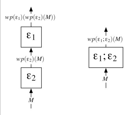
Suppose we take the sequential composition of two operations and , as shown in Fig. 1. For the composed operation and for all predicates we have that
| (21) |
If we calculate weakest preconditions for both operations separately and then compose them sequentially, we obtain
| (22) |
Hence by Eqs.(21) and (22) we obtain that weakest predicate transformers compose sequentially as follows,
| (23) |
This is the same rule as one finds for sequential composition in classical programming languages [Dijkstra76].
Parallel composition.
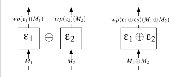
Suppose we take the parallel composition of two operations and , as shown in Fig. 2. For the composed operation we have that
| (24) |
On the other hand, if we calculate weakest preconditions for both operations separately and then compose them in a parallel way, we obtain
| (25) |
Comparing Eqs.(24) and (25) we obtain that for parallel composition weakest precondition predicate transformers compose as follows,
| (26) |
Context extension.
Let us now study what occurs if we weaken a context with dummy classical or quantum variables. Suppose first that we have a QPL program with denotation . We first modify by picking a fresh classical variable and adding it to ’s context; denote the resulting program . The forward semantics of the latter is given by [Selinger03], and hence by Eq.(26) we find that
| (27) |
Suppose next that we add a fresh qubit to ’s context, and write for the resulting program. The forward semantics of is given by
| (28) |
which we write more concisely as
| (29) |
Accordingly, we find that
| (30) |
Iteration.
Consider a flow chart which is obtained from a program by introducing a loop. As explained in the above, the semantics of the flow chart is given by the monoidal trace , where is the semantics of the flow chart obtained from by removing the loop. For a predicate we have that
| (31) |
By iterating explicitly and using Eqs.(17) and (23) we obtain
| (32) |
Comparing Eqs.(31) and (32) we obtain that
| (33) |
Moreover, the existence of the limit in Eq.(33) is guaranteed due to Prop. 1.

Recursion.
Consider an operation which is defined recursively, i.e. an operation satisfying the equation , where is a flow chart. The required fixed point solution to this recursive equation is given by Eqs.(18) and (19). If we work out the weakest precondition relations using Eq.(18) and the fact that weakest precondition predicate transformers are Scott-continuous we obtain
| (34) |
Combining this result with Prop. 6 we find that the weakest precondition predicate transformer for a recursively defined operation is obtained as
| (35) |
The existence of the least upper bound in Eq.(35) is guaranteed by Prop. 1. This result depends of course on the concrete recursive specification considered. Specifically, one needs to determine in order to determine the weakest precondition predicate transformer corresponding to an operation , defined recursively as .
5 Applications
In this section we look at some specific situations and their weakest precondition predicate transformers.
5.1 Grover’s algorithm
We first look into Grover’s algorithm, also known as the database search algorithm [Grover96]. The algorithm is parameterized by the number of qubits and is specified in QPL as follows, where we write for .
| (36) |
Note that we assume the presence of product types of quantum integers – qubit registers of size – and integers , which were elaborated in [Selinger03], and also the presence of integer operations.
The Grover operator is given by
| (37) |
where is a quantum oracle, which labels solutions to the search problem, and is the inversion about mean operation, specifically .
Supposing the solution to the search problem is given by , then the relevant postcondition for Grover is given by , in particular we wish to obtain
| (38) |
where is the final state of the algorithm, and the tuple summation is present due to measurement branching.
We work our way backwards through the algorithm using Eq.(23) in order to find the weakest precondition corresponding to the postcondition . First we derive the weakest precondition for the measurement in the last step of the algorithm. We do this according to a generalization of Eq.(20) for -valued measurements, as follows.
| (39) |
Note that, since the remainder of the algorithm consists of unitary evolution, all relevant preconditions continue to be pure state projectors. In this case Eq.(38) holds only if the output state equals the predicate, that is if , so that pure state preconditions are at the same time the states required for the algorithm to satisfy Eq.(38) after termination.
We now focus in the while loop in the algorithm. Geometrically, the Grover operator is a rotation in the two-dimensional space [Nielsen00, Sec. 6.1.3] spanned by the states and
| (40) |
More specifically, can be decomposed as
| (41) |
Applying again Eq.(23), we obtain as weakest precondition with respect to the while loop the following,
| (42) |
where we omit explicit weakest precondition reasoning for the purely classical command . Using Eq.(41), we see that corresponds to rotations over an angle of in the state space spanned by and . By choosing [Nielsen00, Sec 6.1.3], one rotates the postcondition towards the precondition , where is the initial state of the algorithm, i.e. the equal superposition state, which lies in the space spanned by the states and . In other words, using Eq.(6) and Eq.(38) we obtain that for all
| (43) |
That is, Eq.(38) holds if and only if which is the case by construction of the algorithm. Hence we have established the correctness of the algorithm via our backwards semantics.
We note that an alternative derivation for Grover’s algorithm based on probabilistic weakest preconditions has been reported in [Butler99]. However, the use of probabilistic notions only works there because Grover’s algorithm is considered for pure states only. The mathematical structures underlying their analysis is that of probabilistic weakest preconditions, which are in fact not suited at all for a generalized quantum setting, as we have stressed in Sec. 2. In our setting we could reason about mixed state solutions to Grover and compare them with the pure state solution elaborated in the above. Also, while it may seem at first sight that in [Butler99] the value of is derived via the backward semantics this is in fact not the case. Instead, a recurrence relation for amplitudes occurring in each Grover iteration is solved; these amplitudes are found by applying the Grover iteration backwards, just as we did. We chose to adhere to the interpretation of as a rotation in a two-dimensional state space in order to find ; we could just as well have adhered to the derivation in [Butler99]. While their proof is an ingenious alternative to that in [Nielsen00], it is not based on the theory of probabilistic weakest preconditions.
5.2 Tossing a coin
As a second application, we derive the weakest precondition for the flow chart implementing a fair coin toss [Selinger03, Example 4.1]. In QPL terms the flow chart is specified as follows, where is an input qubit register of unspecified length.
| (44) |
An arbitrary postcondition for this program is of the form , where and are both predicates over and is the number of qubits in the register . We derive the corresponding weakest precondition by flowing backwards through the program, starting with the discard operation. The latter induces the following quantum operation, where is the identity map with as before, 0 denotes the zero block matrix, and is a density matrix in ,
| (45) |
This leads to the following weakest precondition,
| (46) |
Next, we have the measurement step. We just give the result here, as this type of derivation was already encountered in the Grover example above.
| (47) |
The Hadamard transformation is straightforward and leads to
| (48) |
Finally we move through the first command in the coin toss program, namely the addition of a new qubit. The forward semantics of this command is as follows, where is a density matrix in ,
| (49) |
Hence, we obtain the following,
| (50) |
Wrapping all individual steps of the coin toss program up into one weakest precondition predicate transformation according to Eq.(23) we obtain
| (51) |
5.3 Stabilizers are predicates
The stabilizer formalism is an alternative description of quantum states [Gottesman99b]. Instead of describing states as vectors in a suitable Hilbert space, they are described by a set of operators which leave the state invariant. Concretely, for an -qubit system these operators are taken from the Pauli group , i.e. the group of -fold tensor products of the Pauli matrices with factors in front. Note that if we allow all positive operators instead one obtains the more familiar density matrix formalism. Of course not all states can be described in this way. Formally, a stabilizer state is a simultaneous eigenvector of an abelian subgroup of the Pauli group with eigenvalue 1. This subgroup is then called the stabilizer of this state, and usually represented by its generators. Surprisingly, some forms of entanglement, such as graph states for example [Raussendorf02a], as well as all Clifford group operations, can be described efficiently via stabilizers – a celebrated result known as the Gottesman-Knill theorem [Nielsen00, Sec. 10.5.4]. This is because for an -qubit stabilizer state its stabilizer has generators (as opposed to amplitudes in the state formalism). A nice overview of stabilizer theory can be found in [Nielsen00, Ch. 10].
Stabilizers, which are unitaries, fit well within the setting of weakest preconditions, because when restricting ourselves to pure states, they are in fact quantum predicates. This follows from the following theorem.
Proposition 1.
Given a pure state and a unitary we have that
| (52) |
Proof 5.1.
For the left to right direction, we have that
| (53) |
The other direction is obvious.
For example, consider the creation of a Bell state by applying to . The stabilizer of is generated by and . Hence by the above result we have , where is the initial state of the algorithm and for all . Applying Eq.(9), we obtain as weakest preconditions and . By Prop. 6 we thus also have . But then by the above result and are stabilizers of . Hence , as required.
6 Conclusions
In this article, we have developed the predicate transformer and weakest precondition formalism for quantum computation. We have done this by first noting that the quantum analogue to predicates are expectation values of quantum measurements, given by the expression . Then we have defined the concept of weakest preconditions within this framework, proving that a weakest precondition exists for arbitrary completely positive maps and observables. We have also worked out the weakest precondition semantics for the Quantum Programming Language (QPL) developed in [Selinger03]. QPL is the first model for quantum computation with a denotational semantics, and as such the first serious attempt to design a quantum programming language intended for programming quantum algorithms compositionally.
With this development in place one can envisage a goal-directed programming methodology for quantum computation. Of course one needs more experience with quantum programming idioms and the field is not yet ready to produce a “quantum” Science of Programming. It is likely that in the field of communication protocols, such as those based on teleportation, we have a good stock of ideas and examples which could be used as the basis of methodologies in this context.
The most closely related work - apart from Selinger’s work on his programming language - is the work by Sanders and Zuliani [Sanders00] which develops a guarded command language used for developing quantum algorithms. This is a very interesting paper and works seriously towards developing a methodology for quantum algorithms. However, they use probability and nondeterminism to capture probabilistic aspects of quantum algorithms. Ours is an intrinsically quantum framework. The notion of weakest precondition that we develop here is not related to anything in their framework. There are other works [Baltag04] - as yet unpublished - in which a quantum dynamic logic is being developed. Clearly such work will be related though they use a different notion of pairing. Also the work in [Edalat04] is related and merits further investigation. Edalat uses the interval domain of reals rather than the reals as the values of the entries in his density matrices. This seems a good way to deal with uncertainty in the values.
There is a large literature on probabilistic predicate transformers including several papers from the probabilistic systems group at Oxford. A forthcoming book [Morgan04] gives an expository account of their work. We emphasize again that the theory of probabilistic predicate transformers does not capture the proper notions appropriate for the quantum setting. Linearity and complete positivity are essential aspects of the theory of quantum predicate transformers. If one tries to work with probabilistic predicates alone one will not be able to express healthiness conditions that capture the physically allowable transformations, as the example presented in Sec. 3 illustrates.
One might worry that the predicates are too restricted. There are many “observables” in physics that are not positive; for example, the -component of angular momentum, written , for a spin system takes on the values . However, for reasoning about the evolution of one can work instead with the operator which has eigenvalues and and so is a predicate. Of course one cannot do this for unbounded operators like the energy, but this will not be a handicap for quantum computation.
One pleasant aspect of the present work is that it is language independent; though we have used it to give the semantics of QPL the weakest precondition formalism stands on its own. We can therefore apply it to other computational models that are appearing, for example the one-way model [Raussendorf01, Raussendorf02a] for which language ideas are just emerging [Danos04b].
Acknowledgements
It is a pleasure to thank Samson Abramsky, Bob Coecke, Elham Kashefi and Peter Selinger for helpful discussions. Comments by the referees were very helpful.