This thesis provides an explicit construction of a quantum Goppa code for any hyperelliptic curve over a non-binary field. Hyperelliptic curves have conjugate pairs of rational places. We use these pairs to construct self-orthogonal classical Goppa codes with respect to a weighted inner product. These codes are also self-orthogonal with respect to a symplectic inner product and therefore define quantum stabilizer codes. A final transformation leads to a quantum Goppa code with respect to the standard symplectic inner product. Some examples illustrate the described construction.

Furthermore we present a projection of a higher dimensional code onto the base field and a special case when the projected code is again weighted self-orthogonal and symmetric.

Introduction

This diploma thesis uses algebraic geometry, coding theory, and quantum error correction to construct some classes of new quantum Goppa codes. In particular we show that every hyperelliptic curve which has at least one pair of rational places can be used to construct a code. The presented constructions lead to explicit descriptions of quantum error correcting codes. We illustrate all constructions by concrete computations which have been carried out with the help of the computer algebra system Magma [19]. In order to be able to prove properties of these quantum Goppa codes, some basic theory has to be introduced. This thesis does not assume the reader to be familiar with all three different topics and gives brief introductions. It is structured in the following way:

In Chapter 1 the reader gets a short introduction to classical coding theory. The classical Hamming code will serve as an example in which we explain what it means to encode, correct errors, and finally decode codewords.

The basics of quantum mechanics are introduced in Chapter 2. This chapter includes the ideas of quantum information and quantum errors. We will see some general quantum error correcting codes before looking at stabilizer codes, a special kind of quantum codes that can use classical codes for quantum computing. Finally, this chapter shows a way how to transform stabilizer codes in order to make them orthogonal with respect to various symplectic inner products.

Chapter 3 is an introduction to algebraic curves, function fields, divisors, and differentials. The main theorems are the theorem of Riemann-Roch and the strong approximation theorem. It also introduces towers of function fields in order to be able to study the asymptotics of codes. Finally, Goppa codes are defined and we give special properties concerning self-orthogonality.

In Chapter 4, a construction by R. Matsumoto for asymptotically good quantum codes over fields of characteristic two will be presented in detail. His ideas will play an important part in the constructions of the subsequent chapter.

Chapter 5 is the main part of this thesis and gives some new constructions of quantum Goppa codes. We will use hyperelliptic function fields to construct weighted self-orthogonal Goppa codes that can be transformed to symplectic self-orthogonal quantum codes. One method to construct these codes is to use the well known CSS construction. The other method will use a direct construction similar to the one of Chapter 4. Some examples shall help to understand the ideas better.

Finally, Chapter 6 concludes the thesis.

Table of Notations

This section gives an overview over the used symbols and notations.

Notation for Codes

$C$ linear code $d(x,y)$ Hamming distance ${\rm wt}(x)$ weight of $x$ $\dim C$ dimension of code $C$ $\left[n,\,k,\,d\right]$ classical linear code with parameters $n,\,k,\,d$ $d(C)$ minimum distance of $C$ $\langle x,y\rangle$ canonical inner product on $\mathbb{F}_{q}^{n}$ $\langle x,y\rangle^{a}$ inner product with weights $a_{i}$ on $\mathbb{F}_{q}^{n}$ ${\cal G}$ generator matrix of a code $C$ $H$ parity check matrix of a code $C$ $s(x)$ syndrome of $x$ corresponding to a code $C$ $C^{\perp}$ dual code of $C$ $C^{\perp^{a}}$ dual code of $C$ with respect to $\langle\;,\;\rangle^{a}$ $C_{\cal L}(D,G)$ geometric Goppa code associated with $D$ and $G$ $ev_{D}$ evaluation map $C_{\Omega}(D,G)$ Goppa code over differentials associated with $D$ and $G$ $\left[\left[n,\,k,\,d\right]\right]$ quantum stabilizer code with parameters $n,\,k,\,d$ $\langle x,y\rangle_{s}$ symplectic inner product on $\mathbb{F}_{q}^{2n}$ $\langle x,y\rangle_{s}^{a}$ symplectic inner product with weights $a_{i}$ on $\mathbb{F}_{q}^{2n}$ $C^{\perp_{s}}$ symplectic dual code of $C$ $C^{\perp_{s}^{a}}$ symplectic dual code of $C$ with respect to $\langle\;,\;\rangle_{s}^{a}$

Quantum Information Language

$|\psi\rangle$ qudit in ket notation $|b_{1}\ldots b_{n}\rangle$ quantum register in ket notation ${\cal P}$ Pauli group on single qudits ${\cal P}_{n}$ Pauli group on quantum registers of length $n$ $X_{j}$ , $Z_{j}$ generators of the Pauli group $1\hskip-2.5pt\mathrm{l}$ identity operator $H$ Hadamard gate $C-NOT$ controlled-not gate $C-U$ controlled unitary operation $U$ Toffoli Toffoli gate $N(S)$ Normalizer of the stabilizer $S$

Used Algebraic Geometry Terminology

$\mathbb{F}_{q}$ finite field with $q$ elements $\mathbb{F}_{q}^{n}$ $n$ -dimensional vector space over $\mathbb{F}_{q}$ $\mathbb{P}^{2}$ projective space of dimension $2$ $[F^{\prime}:F]$ degree of a field extension $F^{\prime}/F$ $char\,K$ characteristic of $K$ $K[T]$ polynomial ring in one variable over $K$ $K(x)$ rational function field $(f(X,Y,Z))$ ideal spanned by $f(X,Y,Z)$ $F/K$ algebraic function field of one variable ${\cal O}$ valuation ring of $F/K$ $P$ place of $F/K$ $\mathbb{P}_{F}$ set of places of $F/K$ ${\cal O}_{P}$ valuation ring of a place $P$ $v_{P}$ discrete valuation corresponding to $P$ $F_{P}$ residue class field of $P$ $x(P)$ residue class of an element $x\in{\cal O}$ $\deg P$ degree of a place $P$ $P_{\infty}$ infinite place of $K(x)$ ${\cal D}_{F}$ divisor group of $F/K$ ${\rm supp}\,D$ support of the divisor $D$ $D_{1}\leq D_{2}$ ordering of divisors $\deg D$ degree of a divisor $D$ $(x)$ principal divisor of $x$ $(x)_{\infty}$ pole divisor of $x$ ${\cal L}(A)$ space of functions associated with the divisor $A$ $\dim A$ dimension of a divisor $A$ $g$ genus of $F/K$ ${\cal A}_{F}$ adele space of $F/K$ ${\cal A}_{F}(A)$ space of adeles associated with the divisor $A$ $\Omega_{F}$ module of Weil differentials of $F/K$ $\Omega_{F}(A)$ module of Weil differentials associated with the divisor $A$ $(\eta)$ divisor of a Weil differential $\eta\neq 0$ $dx,\;u\,dx$ differentials of $F/K$ $\mathrm{res}_{P}\left(\eta\right)$ residue of a differential $\eta$ at a place $P$ $F^{\sigma}$ fixed field of $\sigma$ $e(P^{\prime}|P)$ ramification index of $P^{\prime}$ over $P$ $f(P^{\prime}|P)$ relative degree of $P^{\prime}$ over $P$ $d(P^{\prime}|P)$ different exponent of $P^{\prime}$ over $P$ $d(P^{\prime})$ different exponent of $P^{\prime}$ if $d(P^{\prime}|P)$ is independent of $P$ ${\rm Diff}(F^{\prime}|F)$ different of $F^{\prime}/F$ ${\rm Gal}(F^{\prime}|F)$ Galois group of $F^{\prime}/F$

Acknowledgements

There are a lot of people who supported me in this work and who have to be thanked.

First, I thank Martin Rötteler for the weekly discussions that helped so much and gave so many ideas. Then I have to thank Raymond Laflamme who gave me the opportunity to work at the Institute for Quantum Computing (IQC) at the University of Waterloo. He, Michele Mosca and the whole institute helped me a lot to integrate in Waterloo and to get an idea of what research means. I thank my office mates, especially Pranab, Niel, and Donny for the mathematical discussions, but also all the others especially for their mental support and motivating words.

Also thanks to Wolfgang K. Seiler and Hans-Peter Butzmann at the Universität Mannheim that they accepted my thesis written in Waterloo and helped me to arrange all formalities in Germany. Thanks to Claus Hertling who proof-read especially the mathematical part of this thesis and gave me helpful hints. And last but not least thanks to Wolfgang Effelsberg who sent me on the exchange program Mannheim - Waterloo and therefore made me meet the people from IQC.

Chapter 1 Classical Coding Theory

Classical codes are used for error correction. Transmission of information over a noisy channel will always cause bit flip errors with a certain probability. When designing a code we try to maximise the number of correctable errors in a codeword and minimise the number of bits we have to send. Interesting math problems arise from the question how to construct families of codes that reach special bounds in their asymptotics. An example for this is the tower of quantum codes constructed in Chapter 5. In general, there are lots of different ideas, how to construct good codes, we will mostly look at codes coming from algebraic geometry.

This chapter gives a short overview over the basic ideas of classical linear codes to introduce the notation used later on. For more information about classical coding theory we refer to [18].

1.1 Linear Codes

Codes do not have to be linear, but if they are linear, many things become easier. Hence we will only use linear codes over finite fields $\mathbb{F}_{q}$ where $q=p^{m}$ is a prime power.

1.1.1 Basic Definitions

Definition 1.1.

A linear code C (over the alphabet $\mathbb{F}_{q}$ ) is a linear subspace of $\mathbb{F}_{q}^{n}$ ; the elements of $C$ are called codewords. We call $n$ the length of $C$ and $\dim C$ (as $\mathbb{F}_{q}$ -vector space) the dimension of $C$ .

Definition 1.2.

For $a=(a_{1},\ldots,a_{n})$ and $b=(b_{1},\ldots,b_{n})\in\mathbb{F}_{q}^{n}$ let

d(a,b):=\left|{\left\{i\;|\;a_{i}\neq b_{i}\right\}}\right|.

This function $d$ is called the Hamming distance on $\mathbb{F}_{q}^{n}$ and defines a metric. The weight of an element $a\in\mathbb{F}_{q}^{n}$ is defined as

{\rm wt}(a):=d(a,0)=\left|{\left\{i\;|\;a_{i}\neq 0\right\}}\right|

Definition 1.3.

The minimum distance $d(C)$ of a linear code $C\neq{\left\{0\right\}}$ is defined as

\displaystyle d(C)

\displaystyle:=

\displaystyle\min{\left\{d(a,b)\;|\;a,b\in C\;\rm{and}\;a\neq b\right\}}=\min{\left\{{\rm wt}(c)\;|\;0\neq c\in C\right\}}.

The second equality holds, because the code is linear and therefore for $a,b\in C$

\displaystyle d(a,b)

\displaystyle=

\displaystyle d(a-b,0)={\rm wt}(a-b)

and $a-b\in C$ because of linearity.

Definition 1.4.

An $\left[n,\,k,\,d\right]$ code is a code of length $n$ and dimension $k$ with minimum distance $d$ (see Definition 1.3) detecting $d-1$ and correcting $t=\left\lfloor\frac{d-1}{2}\right\rfloor$ errors.

1.1.2 Encoding

Definition 1.5.

Let $C$ be an $[n,k]$ code over $\mathbb{F}_{q}$ . A generator matrix ${\cal G}$ of $C$ is a $k\times n$ matrix whose rows form a basis of $C$ , i.e. if ${\left\{c_{1},\ldots,c_{k}\right\}}$ is a basis of $C$ , then

\displaystyle{\cal G}

\displaystyle=

\displaystyle\left(\begin{array}[]{c}c_{1}\\ \vdots\\ c_{k}\end{array}\right)\in\mathbb{F}_{q}^{k\times n}.

Definition 1.6.

The canonical inner product on $\mathbb{F}_{q}^{n}$ is defined by

\langle a,b\rangle:=\sum_{i=1}^{n}a_{i}b_{i}

for $a=(a_{1},\ldots,a_{n})$ and $b=(b_{1},\ldots,b_{n})\in\mathbb{F}_{q}^{n}$ . This is a symmetric bilinear form on $\mathbb{F}_{q}^{n}$ .

Definition 1.7.

If $C\subseteq\mathbb{F}_{q}^{n}$ is a code, then

\displaystyle C^{\perp}

\displaystyle:=

\displaystyle{\left\{u\in\mathbb{F}_{q}^{n}\;|\;\langle u,c\rangle=0\;\rm{for\;all}\;c\in C\right\}}

is called the dual of $C$ . A code $C$ is called self-dual (respectively. self-orthogonal) if $C=C^{\perp}$ (respectively. $C\subseteq C^{\perp}$ ).

Definition 1.8.

A generator matrix $H$ of $C^{\perp}$ is said to be a parity check matrix for $C$ .

Clearly, a parity check matrix of an $\left[n,\,k,\,d\right]$ code $C$ is an $(n-k)\times n$ matrix $H$ of rank $n-k$ , and we have

\displaystyle C

\displaystyle=

\displaystyle{\left\{u\in\mathbb{F}_{q}^{n}\;|\;H\cdot u^{\mathrm{t}}=0\right\}}

1.1.3 Decoding

We can decode linear codes by so-called syndromes. What syndromes are and how to decode with their help will be explained in this section.

Definition 1.9.

The syndrome $s(u)$ of a vector $u\in\mathbb{F}_{q}^{n}$ with respect to a code $C$ is defined by

\displaystyle s(u)

\displaystyle=

\displaystyle u\cdot H^{\mathrm{t}}

where $H^{\mathrm{t}}$ is the transpose of the parity check matrix of $C$ .

By definition of the parity check matrix, we have $\forall c\in C:s(c)=0$ , so that we can characterize $C$ as $C=\{u\in\mathbb{F}_{q}^{n}\;|\;s(u)=0\}$ .

Remark 1.10.

We can divide $\mathbb{F}_{q}^{n}$ into cosets according to the syndromes:

\displaystyle s(u)=s(v)

\displaystyle\Longleftrightarrow

\displaystyle u+C=v+C

This property holds because as seen above, $C$ is the kernel of the linear map that maps every vector to its syndrome with respect to $H$ . We call the vector with the smallest weight in every coset the leader. The leader of a coset need not be unique.

Lemma 1.11.

For a $t$ -error-correcting code $C$ , every vector, whose weight is at most $t$ , is the leader of a coset. This vector is unique and describes the error which has happened during the transmission.

Algorithm 1.12 (Decoding).

1.

For a vector $x\in\mathbb{F}_{q}^{n}$ determine its coset by syndrome calculations.
2.

Find a leader $y$ of its coset. Note that if the coset leader is unique, the decoded vector will be equal to the original one. This is the case if less than $t+1$ errors occurred in a $t$ -error-correcting code (see Lemma 1.11).
3.

Decode $x$ by calculating $x-y$ , which is the wanted vector.

It is known that decision problems corresponding to the general decoding problem are NP-hard [3], also to determine the minimum weight is known to be NP-hard [32]. An (inefficient) decoding strategy is to use look-up tables, especially if many codewords have to be decoded. An overview of possible strategies is given in [2].

1.2 Example: Hamming Code

The following example shows how the whole procedure of encoding and decoding including error correction described in the previous section works.

Definition 1.13.

The Hamming code $C$ is a $\left[7,\,4,\,3\right]$ classical linear code over the field $\mathbb{F}_{2}$ . It has dimension 7, encodes 4 bits and has a minimum distance of 3. That means it can detect 2 errors and correct 1 error.

1.2.1 Encoding

As we have seen above, the generator matrix is a $k\times n$ matrix, so in this example we obtain a $4\times 7$ matrix. It is defined by

\displaystyle{\cal G}

\displaystyle=

\displaystyle\left(\begin{array}[]{rrrrrrr}1&0&1&0&1&0&1\\ 0&1&1&0&0&1&1\\ 0&0&0&1&1&1&1\\ 1&1&1&0&0&0&0\\ \end{array}\right)

This means that our code $C$ is generated by the vectors

(1,0,1,0,1,0,1),\;(0,1,1,0,0,1,1),\;(0,0,0,1,1,1,1),\;\mathrm{and}\;(1,1,1,0,0,0,0),

i.e. it consists of all linear combinations of those 4 vectors over $\mathbb{F}_{2}$ .

Now, from the generator matrix $G$ , we can construct the parity check matrix. This is an $(n-k)\times n$ matrix which consists of the generators of the space orthogonal to $C$ . The rows have to be orthogonal to every row of the generator matrix ( $H\cdot{\cal G}^{t}=0$ ). For our code $C$ the following matrix is one example that satisfies this condition:

H=\left(\begin{array}[]{rrrrrrr}1&0&1&0&1&0&1\\ 0&1&1&0&0&1&1\\ 0&0&0&1&1&1&1\\ \end{array}\right)

If we calculate the matrix product, we get:

\displaystyle H\cdot{\cal G}^{{\mathrm{t}}}

\displaystyle=

\displaystyle\left(\begin{array}[]{rrrrrrr}1&0&1&0&1&0&1\\ 0&1&1&0&0&1&1\\ 0&0&0&1&1&1&1\\ \end{array}\right)\cdot\left(\begin{array}[]{rrrr}1&0&0&1\\ 0&1&0&1\\ 1&1&0&1\\ 0&0&1&0\\ 1&0&1&0\\ 0&1&1&0\\ 1&1&1&0\end{array}\right)={\bf 0}

Transmitting a vector, e.g. $(1,0,1,0)$ , we get its encoding:

\displaystyle(1,0,1,0)\cdot{\cal G}

\displaystyle=

\displaystyle(1,0,1,1,0,1,0)

1.2.2 Decoding

Suppose that a one bit error occurs during the transmission:

(1,0,1,1,0,1,0)\longrightarrow(1,1,1,1,0,1,0)

For error correction we have to calculate the syndrome of the vector:

(1,1,1,1,0,1,0)\cdot H^{t}=(0,1,1)

Now we have to find the leader of the coset $(1,1,1,1,0,1,0)+C$ . To do this, we use the equation:

(a,b,c,d,e,f,g)\cdot H^{t}=(0,1,1)

This equation has the solution $(0,1,0,0,0,0,0)$ . In general we will calculate the leaders once and store them in a look up table. As we know from Lemma 15, a vector is the unique leader of a $t$ correcting code, if it has at most weight $t$ . We have a one error correcting code and $(0,1,0,0,0,0,0)$ has weight one, so it is the unique leader. Then we can correct by calculating:

(1,1,1,1,0,1,0)-(0,1,0,0,0,0,0)=(1,0,1,1,0,1,0)

This gives us back our original codeword. We only have to calculate the linear combination of the rows of $G$ to decode $(1,0,1,1,0,1,0)$ , and we get $(1,0,1,0)$ .

Chapter 2 Quantum Error Correcting Codes

This chapter gives a brief introduction to quantum information and quantum codes. It introduces qudits in general, operations on quantum states, quantum error correcting codes, and stabilizer codes. The relation of this theory to physical models can be found in Appendix A in form of the postulates of quantum mechanics.

2.1 Concepts of Quantum Information

The mathematical foundation of quantum information theory is linear algebra. This section gives the relation between common notations in algebra and its corresponding ones in quantum information.

Definition 2.1.

A qubit is the short form for quantum bit and the analog of a bit in classical computation. The possible states of a quantum bit are the states of the vector space ${\mathbb{C}}^{2}={\cal H}$ . The standard basis of this state space is denoted by

|0\rangle=\left({1\atop 0}\right),\quad|1\rangle=\left({0\atop 1}\right),

where $|\cdot\rangle$ is called the ket notation. The right side denotes the usual vector notation.

The general state of a qubit is a linear combination

\displaystyle|\psi\rangle

\displaystyle=

\displaystyle\alpha|0\rangle+\beta|1\rangle

with $\alpha,\,\beta\in{\mathbb{C}}$ and $\left|\alpha\right|^{2}+\left|\beta\right|^{2}=1$ .

This definition is too restrictive for the following chapters, because the codes we are going to construct will be defined over larger alphabet size than two. Therefore we have to introduce qudits as the generalisation to non-binary systems.

Definition 2.2.

A qudit $|\psi\rangle$ is the generalisation of a qubit. Possible states are the elements of the Hilbert space ${\cal H}={\mathbb{C}}^{d}$ The standard basis for this state space consists of the elements $|0\rangle,\ldots,|d-1\rangle$ and every state can be represented as

\displaystyle|\psi\rangle

\displaystyle=

\displaystyle\sum_{i=0}^{d-1}\alpha_{i}|i\rangle

with $\sum_{i=0}^{d-1}\left|\alpha_{i}\right|^{2}=1$ . In usual vector notation, every qudit $|i\rangle$ corresponds to the $i$ -th vector of unity with one in the $i$ -th component, all other components are zero.

To get consistent definitions and good properties, from now on, we restrict ourselves to $d=p^{m}$ for $m\in{\mathbb{N}}$ .

Definition 2.3.

Let $\omega_{p}=e^{\frac{2\pi i}{p}}$ be a primitive $p$ -th root of unity, then we define the Pauli matrices in the $p$ -ary case by

$\displaystyle X_{j}\|k\rangle=X^{j}\|k\rangle$	$\displaystyle=$	$\displaystyle\|k+j\rangle,$
$\displaystyle Z_{j}\|k\rangle=Z^{j}\|k\rangle$	$\displaystyle=$	$\displaystyle\omega_{p}^{k\cdot j}\|k\rangle,$
$\displaystyle 1\hskip-2.5pt\mathrm{l}\|k\rangle$	$\displaystyle=$	$\displaystyle\|k\rangle$

for $j,k=0,\ldots,d-1$ .

For $d=p^{m}$ with $m>2$ , we have the more general definition

$\displaystyle X_{j}\|k\rangle$	$\displaystyle=$	$\displaystyle\|k+j\rangle,$
$\displaystyle Z_{j}\|k\rangle$	$\displaystyle=$	$\displaystyle\omega_{p}^{{\rm tr}(k\cdot j)}\|k\rangle,$
$\displaystyle 1\hskip-2.5pt\mathrm{l}\|k\rangle$	$\displaystyle=$	$\displaystyle\|k\rangle$

with $\omega_{p}=e^{\frac{2\pi i}{p}}$ for $j,k\in\mathbb{F}_{p^{m}}$ and ${\rm tr}:\mathbb{F}_{p^{m}}\rightarrow\mathbb{F}_{p}$ the trace map from the finite field onto its base field.

Definition 2.4.

The Pauli group for qudits is defined as

{\cal P}=\langle X_{i}Z_{j}|i,j\in\mathbb{F}_{p^{m}}\rangle.

Definition and properties of this group can be found in [10, 12].

Example 2.5.

For the case of qubits we get the well known Pauli matrices

1\hskip-2.5pt\mathrm{l}=\left(\begin{array}[]{rr}1&0\\ 0&1\end{array}\right),\quad X=\left(\begin{array}[]{rr}0&1\\ 1&0\end{array}\right),\quad Z=\left(\begin{array}[]{rr}1&0\\ 0&-1\end{array}\right),\quad Y=\left(\begin{array}[]{rr}0&-1\\ 1&0\end{array}\right)

and the Pauli group consists of the span of these four matrices. It is easy to check that these matrices are all self-inverse. ¹¹ 1 Note that in physics literature instead of $Y$ the matrix $iY$ is used which has the advantage of being hermitian. However, the vector space spanned over the complex numbers is the same.

If we want to generalise these definitions to systems of more than one qubit respectively. qudit, we have to use tensor products of Hilbert spaces in order to get quantum registers.

Definition 2.6.

A quantum register is a multiple qudit system. Its state $|b_{1}\cdots b_{n}\rangle$ is a tensor product of qudits $|b_{i}\rangle$ , $b_{i}\in\mathbb{F}_{p^{m}}$ , i.e.

\displaystyle|b_{1}\cdots b_{n}\rangle

\displaystyle:=

\displaystyle|b_{1}\rangle\otimes\cdots\otimes|b_{n}\rangle.

The state of a quantum register is in the space ${\cal H}^{\otimes n}=({\mathbb{C}}^{d})^{\otimes n}\cong{\mathbb{C}}^{d^{n}}$ and can be written as

\displaystyle|\psi\rangle

\displaystyle=

\displaystyle\sum_{x\in\mathbb{F}_{p^{m}}^{n}}c_{x}|x\rangle

where $c_{x}\in{\mathbb{C}}$ and $\sum_{x\in\mathbb{F}_{p^{m}}^{n}}\left|c_{x}\right|^{2}=1$ .

To be able to use quantum registers, we also have to generalise the operators acting on them.

Definition 2.7.

The Pauli group on a quantum register of length $n$ is the tensor product of the Pauli group on single qubits

\displaystyle{\cal P}_{n}

\displaystyle:=

\displaystyle\langle U_{1}\otimes\cdots\otimes U_{n}|U_{i}\in{\cal P}\;\mathrm{for}\;i=1,\ldots,n\rangle

Every operator acts on the corresponding qudit.

With help of the Pauli group we have already some possible operators that act on qudits respectively. quantum registers, but this will not be sufficient for circuits that we need for quantum error correction. Therefore we will introduce some more important gates. These are defined over $\mathbb{F}_{2}$ .

Definition 2.8.

•

The Hadamard gate $H$ is given by the matrix

$\displaystyle H$ $\displaystyle=$ $\displaystyle\frac{1}{\sqrt{2}}\left(\begin{array}[]{rr}1&1\\ 1&-1\end{array}\right)$

and drawn in the Feynman circuit notation [23] for a qubit $|\psi\rangle$
•

The controlled-not gate $C-NOT$ is given by the matrix

$\displaystyle C-NOT$ $\displaystyle=$ $\displaystyle\left(\begin{array}[]{rrrr}1&0&0&0\\ 0&1&0&0\\ 0&0&0&1\\ 0&0&1&0\end{array}\right)$

and the conventional circuit is denoted by

i.e. the $C-NOT$ is a controlled-X gate.
•

The controlled-U gate $C-U$ is the generalisation of the $C-NOT$ gate for any unitary transformation $U=\left(\begin{array}[]{cc}u_{1}&u_{2}\\ u_{3}&u_{4}\end{array}\right)$ and given by the matrix

$\displaystyle C-U$ $\displaystyle=$ $\displaystyle\left(\begin{array}[]{rrrr}1&0&0&0\\ 0&1&0&0\\ 0&0&u_{1}&u_{2}\\ 0&0&u_{3}&u_{4}\end{array}\right)$

and the conventional circuit notation is

•

The Toffoli gate is a controlled gate with two control and one target bit. This three qubit gate is given by the matrix

\displaystyle{\rm Toffoli}

\displaystyle=

\displaystyle\left(\begin{array}[]{rrrrrrrr}1&0&0&0&0&0&0&0\\ 0&1&0&0&0&0&0&0\\ 0&0&1&0&0&0&0&0\\ 0&0&0&1&0&0&0&0\\ 0&0&0&0&1&0&0&0\\ 0&0&0&0&0&1&0&0\\ 0&0&0&0&0&0&0&1\\ 0&0&0&0&0&0&1&0\\ \end{array}\right)

and its circuit is given by

2.2 Error Model and Quantum Codes in General

In order to construct quantum error correcting codes, we first have to define an error model. An error model tells us what kind of errors appear and what kind of errors we would like to detect or correct.

In the following we will assume that there are no correlated errors, but just errors on single qudits. Errors on single qubits in our error model can be any linear combination of Pauli group elements. We also assume that every qudit is independently affected with the same probability $p$ [15].

We can look at errors as the interaction of a state in a state space $S$ with the environment $Env$ by looking at the total Hilbert space ${\cal H}={\cal H}_{S}\otimes{\cal H}_{Env}$ where ${\cal H}_{S}$ is the Hilbert space of our system and ${\cal H}_{Env}$ is the Hilbert space of the environment. Then an error in its most general form is an operator

E:|\psi\rangle_{S}|0\rangle_{Env}\mapsto\sum_{a\in I}E_{a}|\psi\rangle_{S}|a\rangle_{Env}

where $|a\rangle_{\mathrm{E}nv}$ are some states of the environment and $E_{a}$ acts on our state $|\psi\rangle_{S}$ [23].

Definition 2.9.

A $\left[\left[n,\,k,\,d\right]\right]$ quantum error correcting code (QECC) is a linear code that encodes $k$ qudits into $n$ qudits and is able to detect errors affecting $d-1$ qudits and to correct errors on $\left\lfloor\frac{d-1}{2}\right\rfloor$ qudits.

We cite the following theorem from [14]

Theorem 2.10.

Let $C$ be a subspace of the state space with orthonormal basis ${\left\{|c_{1}\rangle,\ldots,|c_{K}\rangle\right\}}$ . Then $C$ is a quantum error correcting code for the error operators ${\cal E}={\left\{E_{1},\ldots,E_{N}\right\}}$ iff there are constants $\alpha_{k,l}\in{\mathbb{C}}$ such that for all $|c_{i}\rangle,\,|c_{j}\rangle$ and for all $E_{k},\,E_{l}\in{\cal E}$ :

\displaystyle\langle c_{i}|E_{k}^{\dagger}E_{l}|c_{j}\rangle

\displaystyle=

\displaystyle\delta_{i,j}\alpha_{k,l}.

This theorem tells us that errors have to act on the states by mapping them into orthogonal subspaces of the state space in order to be able to recover the state.

For our error model it suffices to correct so called dit and phase errors. Dit errors are bit flip errors in the binary case and given by the acting of the $X$ gate on the state. Phase flip errors occur when the $Z$ operator is applied to our state.

Definition 2.11.

A bit flip error is given by the following mapping:

	$\displaystyle\|0\rangle$	$\displaystyle\mapsto$	$\displaystyle\|1\rangle$
	$\displaystyle\|1\rangle$	$\displaystyle\mapsto$	$\displaystyle\|0\rangle$

Similarly the phase error acts on a qubit:

	$\displaystyle\|0\rangle$	$\displaystyle\mapsto$	$\displaystyle\|0\rangle$
	$\displaystyle\|1\rangle$	$\displaystyle\mapsto$	$\displaystyle-\|1\rangle$

More generally dit errors are given by the operators $X_{\alpha}$ and phase errors by the operators $Z_{\beta}$ as in Definition 2.3.

Theorem 2.12.

For correction of independent errors on single qudits, it suffices to correct dit and phase flip errors, i.e. the set

{\cal P}={\left\{X_{\alpha}Z_{\beta}\;|\;\alpha,\beta\in\mathbb{F}_{p^{m}}\right\}}

forms an orthonormal basis for the set of matrices acting on one qudit, ${\mathbb{C}}^{p^{m}\times p^{m}}$ with respect to the matrix inner product $\langle A,B\rangle=\frac{1}{p^{m}}\,{\rm tr}(A^{\dagger}B)$ .

Proof.

If we can show that for all $\alpha_{i},\beta_{j}\in\mathbb{F}_{p^{m}}$

\displaystyle\langle X_{\alpha_{1}}Z_{\beta_{1}},X_{\alpha_{2}}Z_{\beta_{2}}\rangle

\displaystyle=

\displaystyle\delta_{(\alpha_{1},\beta_{1}),(\alpha_{2},\beta_{2})},

these operators have to form a basis, because

\displaystyle\left|{\cal P}\right|

\displaystyle=

\displaystyle(p^{m})^{2}=\dim{\mathbb{C}}^{p^{m}\times p^{m}}

Let $X_{\alpha_{1}}Z_{\beta_{1}}$ and $X_{\alpha_{2}}Z_{\beta_{2}}$ be two arbitrary elements of ${\cal P}$ , then

$\displaystyle\langle X_{\alpha_{1}}Z_{\beta_{1}},X_{\alpha_{2}}Z_{\beta_{2}}\rangle$	$\displaystyle=$	$\displaystyle\frac{1}{p^{m}}{\rm tr}((X_{\alpha_{2}}Z_{\beta_{2}})^{\dagger}X_{\alpha_{1}}Z_{\beta_{1}})$
	$\displaystyle=$	$\displaystyle\frac{1}{p^{m}}{\rm tr}(Z_{\beta_{2}}^{\dagger}X_{\alpha_{2}}^{\dagger}X_{\alpha_{1}}Z_{\beta_{1}})$
	$\displaystyle=$	$\displaystyle\frac{1}{p^{m}}{\rm tr}(Z_{-\beta_{2}}X_{-\alpha_{2}}X_{\alpha_{1}}Z_{\beta_{1}})$
	$\displaystyle=$	$\displaystyle\frac{1}{p^{m}}{\rm tr}(Z_{-\beta_{2}}X_{\alpha_{1}-\alpha_{2}}Z_{\beta_{1}})$
	$\displaystyle=$	$\displaystyle\frac{1}{p^{m}}{\rm tr}(X_{\alpha_{1}-\alpha_{2}}Z_{\beta_{1}-\beta_{2}})$

Note that $Z_{\alpha}$ has nothing but diagonal terms for any $\alpha$ and $X_{\alpha}$ has no diagonal terms if $\alpha\neq 0$ . So we can conclude

•

if $\alpha_{1}\neq\alpha_{2}$ , ${\rm tr}(X_{\alpha_{1}-\alpha_{2}}Z_{\beta_{1}-\beta_{2}})=0$ and the two elements are orthogonal

•

if $\alpha_{1}=\alpha_{2}$ ,

\displaystyle\langle X_{\alpha_{1}}Z_{\beta_{1}},X_{\alpha_{2}}Z_{\beta_{2}}\rangle

\displaystyle=

\displaystyle\frac{1}{p^{m}}{\rm tr}(Z_{\beta_{1}-\beta_{2}})

–

if $\beta_{1}=\beta_{2}$ , $\langle X_{\alpha_{1}}Z_{\beta_{1}},X_{\alpha_{2}}Z_{\beta_{2}}\rangle=\frac{1}{p^{m}}{\rm tr}(1\hskip-2.5pt\mathrm{l})=\frac{1}{p^{m}}\cdot p^{m}=1$

–

if $\beta_{1}\neq\beta_{2}$ ,

\displaystyle\langle X_{\alpha_{1}}Z_{\beta_{1}},X_{\alpha_{2}}Z_{\beta_{2}}\rangle

\displaystyle=

\displaystyle\frac{1}{p^{m}}{\rm tr}(Z_{\beta_{1}-\beta_{2}})=\frac{1}{p^{m}}\sum_{z\in\mathbb{F}_{p^{m}}}\omega_{p}^{{\rm tr}((\beta_{1}-\beta_{2})z)}=0

Therefore the two operators are orthogonal.

∎

In the following we will give an example of a simple quantum code which is also known as repetition code. The difference to the classical repetition code is that we cannot copy states:

Theorem 2.13 (No-Cloning Theorem [23]).

It is not possible to copy arbitrary quantum states.

Proof.

Assume there exists a unitary operation $U$ that copies arbitrary quantum states. Let $|\psi\rangle$ and $|\phi\rangle$ be arbitrary states. Then

	$\displaystyle U(\|\psi\rangle\otimes\|s\rangle)$	$\displaystyle=$	$\displaystyle\|\psi\rangle\otimes\|\psi\rangle$
	$\displaystyle U(\|\phi\rangle\otimes\|s\rangle)$	$\displaystyle=$	$\displaystyle\|\phi\rangle\otimes\|\phi\rangle.$

The inner product of these two equations gives

\displaystyle\langle\psi|\phi\rangle

\displaystyle=

\displaystyle\langle\psi|\phi\rangle^{2}.

Hence cloning of unknown states is not possible. ∎

Therefore we have to use the properties of linear algebra. These examples can for example be reviewed in [11, 15].

Example 2.14 (Repetition Code for Bit Flips).

The easiest way to correct one error in classical coding theory is the repetition code, that maps

	$\displaystyle 0$	$\displaystyle\mapsto$	$\displaystyle 000,$
	$\displaystyle 1$	$\displaystyle\mapsto$	$\displaystyle 111.$

Decoding is performed by correcting the most likely error. In this case, we will decode with the majority principle, e.g.

	$\displaystyle 001$	$\displaystyle\stackrel{{\scriptstyle decoding}}{{\Longrightarrow}}$	$\displaystyle 000,$
	$\displaystyle 101$	$\displaystyle\stackrel{{\scriptstyle decoding}}{{\Longrightarrow}}$	$\displaystyle 111.$

The problem with this code in quantum error correction is that we cannot copy arbitrary quantum states (see Theorem 2.13). However, we can do something similar to the classical repetition code. First, we will look at bit flips and imitate the classical code. Then in the next example, we will transform the code such that it can correct phase errors.

Let us encode one qubit into three, i.e.

	$\displaystyle\|0\rangle$	$\displaystyle\mapsto$	$\displaystyle\|000\rangle,$
	$\displaystyle\|1\rangle$	$\displaystyle\mapsto$	$\displaystyle\|111\rangle.$

Then an arbitrary superposition will be encoded as

\displaystyle\alpha|0\rangle+\beta|1\rangle

\displaystyle\mapsto

\displaystyle\alpha|000\rangle+\beta|111\rangle.

In the following we will assume that a bit flip error occurred on the first qubit. This is sufficient, because of the symmetry of the code, all calculations will be the same for an error on one of the other qubits.

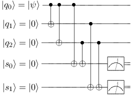
An error on the first qubit will map the state $\alpha|000\rangle+\beta|111\rangle$ to $\alpha|100\rangle+\beta|011\rangle$ . This error can be detected with two ancilla qubits by parity check. Let the ancilla qubits be in the state $|0\rangle$ , then we use two C-NOT gates on every ancilla qubit like in Figure 2.1 and get

$\displaystyle\|000\rangle\|00\rangle$	$\displaystyle\mapsto$	$\displaystyle\|000\rangle\|00\rangle,$
$\displaystyle\|100\rangle\|00\rangle$	$\displaystyle\mapsto$	$\displaystyle\|100\rangle\|10\rangle,$
$\displaystyle\|010\rangle\|00\rangle$	$\displaystyle\mapsto$	$\displaystyle\|010\rangle\|01\rangle,$
$\displaystyle\|001\rangle\|00\rangle$	$\displaystyle\mapsto$	$\displaystyle\|001\rangle\|11\rangle,$
$\displaystyle\|111\rangle\|00\rangle$	$\displaystyle\mapsto$	$\displaystyle\|111\rangle\|00\rangle,$
$\displaystyle\|011\rangle\|00\rangle$	$\displaystyle\mapsto$	$\displaystyle\|011\rangle\|10\rangle,$
$\displaystyle\|101\rangle\|00\rangle$	$\displaystyle\mapsto$	$\displaystyle\|101\rangle\|01\rangle,$
$\displaystyle\|110\rangle\|00\rangle$	$\displaystyle\mapsto$	$\displaystyle\|110\rangle\|11\rangle.$

If we measure the ancilla bits, we will deterministically get syndrome bits 0 or 1 and can uniquely assign it to the single bit flip error that has occurred.

Refer to caption — Figure 2.1: Encoding and syndrome measurement circuit for the repetition bit flip code with code bits $|q_{0}\rangle=|\psi\rangle,\;|q_{1}\rangle,\;|q_{2}\rangle$ and syndrome bits $|s_{0}\rangle,\;|s_{1}\rangle$ .

Example 2.15 (Repetition Code for Phase Errors).

The important observation for phase correction is that bit flip errors transform to phase errors under the Hadamard transformation and vice versa. So we encode

	$\displaystyle\|0\rangle$	$\displaystyle\mapsto$	$\displaystyle\frac{1}{\sqrt{2^{3}}}(\|0\rangle+\|1\rangle)(\|0\rangle+\|1\rangle)(\|0\rangle+\|1\rangle)=:\|{+++}\rangle$
	$\displaystyle\|1\rangle$	$\displaystyle\mapsto$	$\displaystyle\frac{1}{\sqrt{2^{3}}}(\|0\rangle-\|1\rangle)(\|0\rangle-\|1\rangle)(\|0\rangle-\|1\rangle)=:\|{---}\rangle$

and a phase error on the first qubit will map

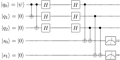
	$\displaystyle\|{+++}\rangle$	$\displaystyle\mapsto$	$\displaystyle\|{-++}\rangle$
	$\displaystyle\|{---}\rangle$	$\displaystyle\mapsto$	$\displaystyle\|{+--}\rangle$

We can detect these errors by Hadamard transformation to the standard basis and the same syndrome calculations as before. Then we apply another Hadamard and perform the necessary error corrections. The complete circuit of this encoding and decoding process is given in Figure 2.2.

The combination of these two codes gives our first quantum code, known as Shor code [25], encoding one qubit into nine and being able to correct bit and phase flip errors and therefore any error on single qubits. This code is a $\left[\left[9,\,1,\,3\right]\right]$ code.

Example 2.16 (9-qubit code).

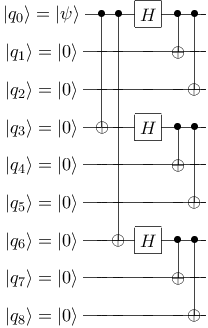
If we concatenate the codes given in Examples 2.14 and 2.15, we get a code that can correct bit and phase flip errors on one qubit. Therefore we encode

$\displaystyle\|0\rangle$	$\displaystyle\mapsto$	$\displaystyle\frac{1}{\sqrt{2^{3}}}(\|000\rangle+\|111\rangle)(\|000\rangle+\|111\rangle)(\|000\rangle+\|111\rangle)$
	$\displaystyle=$	$\displaystyle\frac{1}{\sqrt{2^{3}}}(\|000000000\rangle+\|000000111\rangle+\|000111000\rangle+\|000111111\rangle$
		$\displaystyle+\|111000000\rangle+\|111000111\rangle+\|111111000\rangle+\|111111111\rangle)$
	$\displaystyle=$	$\displaystyle\|\bar{0}\rangle$
$\displaystyle\|1\rangle$	$\displaystyle\mapsto$	$\displaystyle\frac{1}{\sqrt{2^{3}}}(\|000\rangle-\|111\rangle)(\|000\rangle-\|111\rangle)(\|000\rangle-\|111\rangle)$
	$\displaystyle=$	$\displaystyle\frac{1}{\sqrt{2^{3}}}(\|000000000\rangle-\|000000111\rangle-\|000111000\rangle+\|000111111\rangle$
		$\displaystyle-\|111000000\rangle+\|111000111\rangle+\|111111000\rangle-\|111111111\rangle)$
	$\displaystyle=$	$\displaystyle\|\bar{1}\rangle$

Then bit flip errors can be corrected in blocks of three qubits, phase flip errors in the comparison of the three qubit blocks. The circuit for this encoding is given in Figure 2.3.

2.3 Stabilizer Codes

Stabilizer codes were introduced by Daniel Gottesman [8]. This type of quantum error correction is very useful since it allows us to reuse results from classical coding theory and to describe a large class of quantum codes.

2.3.1 Basic Definitions

In the last section we saw that it is sufficient to correct dit and phase errors. The idea of a stabilizer code is to define a commuting set of Pauli operators and use the set of states that is invariant under these operators as code space, i.e. the code is the +1 eigenspace of all the operators.

Recall that two operators $E,F$ commute iff $EF=FE$ .

Definition 2.17.

A Stabilizer code $S$ of length $n$ is an Abelian subgroup of the Pauli group ${\cal P}_{n}$ . Codewords are the states of the state space that are invariant under all elements of $S$ .

Remark 2.18.

An important feature of stabilizer codes is that the stabilizer forms an Abelian group. Error detection and correction takes place by measuring commutation and anti-commutation of operators.

First we will look at the commutation behaviour of single qudit operators in the $p$ -ary case. It is easy to show that $X^{\alpha}$ commutes with $X^{\beta}$ . Similarly $Z^{\alpha}$ commutes with $Z^{\beta}$ .

The problem is what happens with $X^{\alpha}$ and $Z^{\beta}$ . It suffices to show what happens with $X$ and $Z$ , because we can split $X^{\alpha}$ into $X\cdot X\cdots X$ . In general, in case $p$ prime $X$ is given by the matrix

\displaystyle X

\displaystyle=

\displaystyle\left(\begin{array}[]{ccccc}0&0&\cdots&0&1\\ 1&0&\cdots&0&0\\ 0&1&\cdots&0&0\\ \vdots&\vdots&\ddots&\vdots&\vdots\\ 0&0&\cdots&1&0\\ \end{array}\right).

The matrix for $Z$ looks like

\displaystyle Z

\displaystyle=

\displaystyle\left(\begin{array}[]{cccc}1&0&\cdots&0\\ 0&\omega_{p}&\cdots&0\\ \vdots&\vdots&\ddots&\vdots\\ 0&0&\cdots&\omega_{p}^{p-1}\\ \end{array}\right).

Then

\displaystyle XZ

\displaystyle=

\displaystyle\left(\begin{array}[]{ccccc}0&0&\cdots&0&\omega_{p}^{p-1}\\ 1&0&\cdots&0&0\\ 0&\omega_{p}&\cdots&0&0\\ \vdots&\vdots&\ddots&\vdots&\vdots\\ 0&0&\cdots&\omega_{p}^{p-2}&0\\ \end{array}\right)

and

\displaystyle ZX

\displaystyle=

\displaystyle\left(\begin{array}[]{ccccc}0&0&\cdots&0&1\\ \omega_{p}&0&\cdots&0&0\\ 0&\omega_{p}^{2}&\cdots&0&0\\ \vdots&\vdots&\ddots&\vdots&\vdots\\ 0&0&\cdots&\omega_{p}^{p-1}&0\\ \end{array}\right)=\omega_{p}XZ.

So we get for $X^{\alpha}$ and $Z^{\beta}$ , $\alpha,\beta\in\mathbb{F}_{p}$

\displaystyle Z^{\beta}X^{\alpha}

\displaystyle=

\displaystyle\omega_{p}^{\alpha\cdot\beta}X^{\alpha}Z^{\beta}.

In the case of a field $\mathbb{F}_{p^{m}}$ we get for $\alpha,\beta\in\mathbb{F}_{p^{m}}$

\displaystyle Z_{\beta}X_{\alpha}

\displaystyle=

\displaystyle\omega_{p}^{{\rm tr}(\alpha\cdot\beta)}X_{\alpha}Z_{\beta}.

Since we have defined the commutation rules on a single qudit operator, we can generalise this to operators on quantum registers. Hence for two operators

U_{1}=X_{\alpha_{1}}Z_{\beta_{1}}\otimes\cdots\otimes X_{\alpha_{n}}Z_{\beta_{n}},\quad U_{2}=X_{\mu_{1}}Z_{\nu_{1}}\otimes\cdots\otimes X_{\mu_{n}}Z_{\nu_{n}}

we have that

\displaystyle U_{2}\cdot U_{1}

\displaystyle=

\displaystyle\omega_{p}^{\sum_{i=1}^{n}\alpha_{i}\nu_{i}-\mu_{i}\beta_{i}}U_{1}\cdot U_{2}

in case $p$ prime and therefore two operators commute iff

\displaystyle\sum_{i=1}^{n}\alpha_{i}\nu_{i}-\mu_{i}\beta_{i}

\displaystyle=

\displaystyle 0.

In the case of a field $\mathbb{F}_{p^{m}}$ with $m\geq 2$ , we get

\displaystyle U_{2}\cdot U_{1}

\displaystyle=

\displaystyle\omega_{p}^{\sum_{i=1}^{n}{\rm tr}(\alpha_{i}\nu_{i}-\mu_{i}\beta_{i})}U_{1}\cdot U_{2}

and therefore two operators commute iff

\displaystyle\sum_{i=1}^{n}{\rm tr}(\alpha_{i}\nu_{i}-\mu_{i}\beta_{i})

\displaystyle=

\displaystyle 0.

Corollary 2.19.

Let $S$ be a stabilizer, i.e. an Abelian subgroup of ${\cal P}_{n}$ . If a state $|\psi\rangle$ is in the +1 eigenspace of a set of generators ${\left\{G_{1},\ldots,G_{l}\right\}}$ of $S$ , it is an eigenstate of all elements in $S$ .

Proof.

An arbitrary element $F\in S$ is a linear combination of the set of generators:

$\displaystyle F\|\psi\rangle$	$\displaystyle=$	$\displaystyle(G_{1}^{\alpha_{1}}\cdots G_{l}^{\alpha_{l}})\|\psi\rangle$
	$\displaystyle=$	$\displaystyle(G_{1}^{\alpha_{1}}\cdots G_{l-1}^{\alpha_{l-1}})\,G_{l}^{\alpha_{l}}\,\|\psi\rangle$
	$\displaystyle=$	$\displaystyle(G_{1}^{\alpha_{1}}\cdots G_{l-1}^{\alpha_{l-1}})\|\psi\rangle$
	$\displaystyle=$	$\displaystyle\cdots$
	$\displaystyle=$	$\displaystyle\|\psi\rangle$

for any $|\psi\rangle$ that is in the +1 eigenspace of the set of generators and $\alpha_{i}\in\mathbb{F}_{p^{m}}$ for all $i$ . Therefore $|\psi\rangle$ is in the +1 eigenspace of $F$ . ∎

Lemma 2.20.

The stabilizer $S$ of a stabilizer code is an Abelian group, i.e. all stabilizer elements commute.

Proof.

Assume that not all of them commute, then there exist $E,F\in S$ with $EF=\omega_{p}^{\alpha}FE$ where $\alpha\neq 0$ . So all states $|\psi\rangle$ in the code satisfy

	$\displaystyle\|\psi\rangle$	$\displaystyle=$	$\displaystyle EF\|\psi\rangle=\omega_{p}^{\alpha}FE\|\psi\rangle$
		$\displaystyle=$	$\displaystyle\omega_{p}^{\alpha}\|\psi\rangle$

So it has eigenvalue +1 and $\omega_{p}^{\alpha}$ at the same time and therefore contradiction. ∎

Since we have seen that it suffices to look at a set of generators, we can represent a stabilizer code in an easier way:

Definition 2.21.

A generator matrix ${\cal G}$ of a stabilizer code is an $l\times 2n$ -matrix

\displaystyle{\cal G}

\displaystyle=

\displaystyle\left(X|Z\right)

where the first $n$ components represent the $X$ errors, the second $n$ components the $Z$ errors. This matrix defines a $\left[\left[n,\,k,\,d\right]\right]$ quantum error correcting code with $k=n-l$ .

Lemma 2.22.

Elements $x=(x_{1},\ldots,x_{2n}),\;y=(y_{1},\ldots,y_{2n})$ of the Pauli group commute in the vector representation, i.e. $(x_{1},\ldots,x_{2n})$ means $X_{x_{1}}Z_{x_{n+1}}\otimes\cdots\otimes X_{x_{n}}Z_{x_{2n}}$ , if

\langle x,y\rangle_{s}=\sum_{i=1}^{n}x_{i}y_{n+i}-x_{n+i}y_{i}=0.

We call $\langle x,y\rangle_{s}$ the standard symplectic inner product.

Proof.

A vector $(x_{1},\ldots,x_{2n})$ in this representation denotes the operator

X_{x_{1}}Z_{x_{n+1}}\otimes\cdots\otimes X_{x_{n}}Z_{x_{2n}}.

Therefore we get

	$\displaystyle(X_{y_{1}}Z_{y_{n+1}}\otimes\cdots\otimes X_{y_{n}}Z_{y_{2n}})(X_{x_{1}}Z_{x_{n+1}}\otimes\cdots\otimes X_{x_{n}}Z_{x_{2n}})$
	$\displaystyle=\omega_{p}^{{\rm tr}(\sum_{i=1}^{n}x_{i}y_{n+i}-x_{n+i}y_{i})}(X_{x_{1}}Z_{x_{n+1}}\otimes\cdots)(X_{y_{1}}Z_{y_{n+1}}\otimes\cdots\otimes X_{y_{n}}Z_{y_{2n}})$
	$\displaystyle=\omega_{p}^{{\rm tr}(0)}(X_{x_{1}}Z_{x_{n+1}}\otimes\cdots\otimes X_{x_{n}}Z_{x_{2n}})(X_{y_{1}}Z_{y_{n+1}}\otimes\cdots\otimes X_{y_{n}}Z_{y_{2n}})$
	$\displaystyle=(X_{x_{1}}Z_{x_{n+1}}\otimes\cdots\otimes X_{x_{n}}Z_{x_{2n}})(X_{y_{1}}Z_{y_{n+1}}\otimes\cdots\otimes X_{y_{n}}Z_{y_{2n}})$

and therefore the operators commute. ∎

Example 2.23.

If $S$ is generated by $XYI=X\otimes Y\otimes 1\hskip-2.5pt\mathrm{l}$ and $ZXX=Z\otimes X\otimes X$ over $\mathbb{F}_{2}$ , the generator matrix is given by

\displaystyle{\cal G}

\displaystyle=

\displaystyle\left(\begin{array}[]{ccc|ccc}1&1&0&0&1&0\\ 0&1&1&1&0&0\end{array}\right)

Let $x=\left(\begin{array}[]{ccc|ccc}1&1&0&0&1&0\end{array}\right)$ and $y=\left(\begin{array}[]{ccc|ccc}0&1&1&1&0&0\end{array}\right)$ , then

	$\displaystyle\langle x,y\rangle_{s}$	$\displaystyle=$	$\displaystyle(1\cdot 1+1\cdot 0+0\cdot 0)-(0\cdot 0+1\cdot 1+1\cdot 0)$
		$\displaystyle=$	$\displaystyle 1-1=0$

We already introduced the 9-qubit code in the previous section. In the following we give a description in terms of stabilizers.

Example 2.24.

9-qubit code

The 9-qubit code encodes one qubit into 9. Therefore our generator matrix will have size $8\times 18$ .

Claim

	$\displaystyle{\cal G}$	$\displaystyle=$	$\displaystyle\left(\begin{array}[]{ccccccccc}Z&Z&0&0&0&0&0&0&0\\ Z&0&Z&0&0&0&0&0&0\\ 0&0&0&Z&Z&0&0&0&0\\ 0&0&0&Z&0&Z&0&0&0\\ 0&0&0&0&0&0&Z&Z&0\\ 0&0&0&0&0&0&Z&0&Z\\ X&X&X&X&X&X&0&0&0\\ X&X&X&0&0&0&X&X&X\end{array}\right)$
		$\displaystyle=$	$\displaystyle\left(\begin{array}[]{ccccccccc\|ccccccccc}0&0&0&0&0&0&0&0&0&1&1&0&0&0&0&0&0&0\\ 0&0&0&0&0&0&0&0&0&1&0&1&0&0&0&0&0&0\\ 0&0&0&0&0&0&0&0&0&0&0&0&1&1&0&0&0&0\\ 0&0&0&0&0&0&0&0&0&0&0&0&1&0&1&0&0&0\\ 0&0&0&0&0&0&0&0&0&0&0&0&0&0&0&1&1&0\\ 0&0&0&0&0&0&0&0&0&0&0&0&0&0&0&1&0&1\\ 1&1&1&1&1&1&0&0&0&0&0&0&0&0&0&0&0&0\\ 1&1&1&0&0&0&1&1&1&0&0&0&0&0&0&0&0&0\\ \end{array}\right)$

is a generator matrix for the stabilizer code of the 9-qubit code.

Proof.

It is easy to check that the codewords are invariant under ${\cal G}$ and as ${\cal G}$ has rang 8, it has to be a generator matrix for the code. ∎

2.3.2 Error Detection and Correction

Like in classical coding theory we can detect and correct errors by syndrome measurements, but in the quantum case we are not allowed to measure the state, because this in general will destroy the superposition (see A).

Definition 2.25.

An ancilla qudit is an extra qudit that is used during computations, but is not part of the input or output, and is prepared in some fixed state, usually $|0\rangle$ .

Before we can introduce error correction and the amount of errors we can correct and detect, we have to define some more terms like weight and distance for quantum codes.

Definition 2.26.

The weight $wt$ of an operator $U_{1}\otimes\cdots\otimes U_{n}$ is the number of elements $U_{i}$ that are not equal to the identity, e.g.

X\otimes 1\hskip-2.5pt\mathrm{l}\otimes 1\hskip-2.5pt\mathrm{l}\otimes Z\otimes Z

has weight 3.

In classical coding theory the distance of a stabilizer code (which is a linear code) would be the minimal weight over all codewords. In the quantum case this does not hold like that, because we have to detect different types of errors.

Definition 2.27.

The normalizer $N(S)$ of a stabilizer $S$ is the set of Pauli operators that commute with all stabilizer elements.

\displaystyle N(S)

\displaystyle=

\displaystyle{\left\{F\in{\cal P}_{n}\;|\;EF=FE\quad\forall E\in S\right\}}.

This definition allows us to distinguish between three different types of errors.

Lemma 2.28.

Let $F\in{\cal P}_{n}$ be an error operator. Then the following three cases are possible:

1.

If $F\in S$ nothing happened to the code.
2.

If $F\in{\cal P}_{n}\backslash N(S)$ the error is detectable and can be corrected with the most likely error principle (see 1.10 and 1.11).
3.

If $F\in N(S)\backslash S$ the error cannot be detected and therefore is not correctable.

Proof.

Let $|\psi\rangle$ be any element of the code. Then $E|\psi\rangle=|\psi\rangle$ for all $E\in S$ .

1.

If $F\in S$ , we get for all codewords

$\displaystyle F|\psi\rangle$ $\displaystyle=$ $\displaystyle|\psi\rangle$

and nothing happens to the codeword.

If $F\in{\cal P}_{n}\backslash N(S)$ for all $E\in S$

	$\displaystyle E(F\|\psi\rangle)$	$\displaystyle=$	$\displaystyle(EF)\|\psi\rangle=(\omega_{p}^{\alpha}FE)\|\psi\rangle$
		$\displaystyle=$	$\displaystyle\omega_{p}^{\alpha}F\|\psi\rangle$

Therefore the faulty codeword is in the $\omega_{p}^{\alpha}$ eigenspace and detectable by syndrome measurements. With the method introduced in Chapter 1 it is correctable up to half the distance.

If $F\in N(S)\backslash S$ for all $E\in S$

	$\displaystyle E(F\|\psi\rangle)$	$\displaystyle=$	$\displaystyle(EF)\|\psi\rangle=(FE)\|\psi\rangle$
		$\displaystyle=$	$\displaystyle F\|\psi\rangle$

and so we cannot detect the error by syndrome measurement, because $F|\psi\rangle$ is also in the $+1$ eigenspace.

∎

This lemma allows us to introduce the distance of a stabilizer code.

Definition 2.29.

The distance $d$ of a quantum stabilizer code $C$ is the minimum weight of all normalizer elements that are not in the stabilizer.

\displaystyle d

\displaystyle=

\displaystyle\min{\left\{wt(x)\;|\;x\in N(S)\backslash S\right\}}.

In other words, if we denote the normalizer as the set of all operators that commute with all elements in the stabilizer, then the normalizer is equal to the dual code $C^{\perp_{s}}$ with respect to the symplectic inner product $\langle\,,\,\rangle_{s}$ . We obtain that

\displaystyle d

\displaystyle=

\displaystyle\min{\left\{wt(x)\;|\;x\in C^{\perp_{s}}\backslash C\right\}}.

To be able to correct errors smaller than $\left\lfloor\frac{d-1}{2}\right\rfloor$ as in classical coding theory, we can use syndrome measurements.

Algorithm 2.30.

1.

Let $x_{1},\ldots,x_{l}$ be the generators of the stabilizer code, i.e. the rows of the generator matrix.
2.

Prepare $l$ ancilla dits in the $|+\rangle=\frac{1}{\sqrt{2}}(|0\rangle+|1\rangle)$ state. Every ancilla bit corresponds to one stabilizer generator.
3.

Perform controlled operations for every stabilizer generator as in Figure 2.4, i.e. if

$\displaystyle U^{(i)}$ $\displaystyle=$ $\displaystyle U^{(i)}_{1}\otimes\cdots\otimes U^{(i)}_{n},$

perform controlled $U^{(i)}_{j}$ operations on the $j$ th qubit.

Figure 2.4: Example of a syndrome measurement in case where the stabilizer is given by the two generators $U^{(1)}_{1}\otimes\cdots\otimes U^{(1)}_{n}$ and $U^{(2)}_{1}\otimes\cdots\otimes U^{(2)}_{n}$
4.

Measure the ancilla dits. The results are our syndromes.
5.

Use classical theory (see Chapter 1) to determine the errors.
6.

Apply the necessary gates to correct the errors.

Note that this algorithm uses measurements and error detection and correction are assumed to be perfect. Algorithm 2.30 is not fault-tolerant, however, it has been shown how to make syndrome measurements fault-tolerant for any stabilizer code [9]. One example how to omit measurements is given by Example 2.31 below.

Example 2.31.

In Example 2.14 we saw how to correct bit flip errors. In order to be able to locate errors, we had to measure the syndrome bits. An automatic error correction can be achieved by the circuit given in Figure 2.5. There we use a Toffoli gate to correct errors.

A correction without measurement is in general possible if we use fresh ancilla qubits every time error correction is performed (see Box 10.1 in [23]).

2.3.3 Weighted Symplectic Inner Product

In the following chapters we will see that our construction does not always give codes that are orthogonal with respect to the standard symplectic inner product. However, we can construct codes $C$ which are orthogonal with respect to

\displaystyle\langle x,y\rangle_{s}^{a}

\displaystyle:=

\displaystyle\sum_{i=0}^{c}4na_{i}(x_{i}\,y_{n+i}-x_{n+i}\,y_{i})=0

for all $x,y\in C$ and all $a_{i}\neq 0$ . We will call it weighted symplectic inner product.

The following lemma shows that we can construct a stabilizer code with respect to the standard symplectic inner product with the same properties as the old one with respect to the special symplectic inner product.

Lemma 2.32.

Let $C$ be a linear code over $\mathbb{F}_{p^{m}}$ which is self-orthogonal with respect to the weighted symplectic inner product $\langle\;,\,\rangle_{s}^{a}$ and has a corresponding quantum code with parameters $\left[\left[n,\,k,\,d\right]\right]$ and generator matrix

{\cal G}=\left(\begin{array}[]{ccc|ccc}c_{1,1}&\cdots&{c_{1,n}}&{c_{1,n+1}}&\cdots&{c_{1,2n}}\\ \vdots&\ddots&\vdots&\vdots&\ddots&\vdots\\ {c_{l,1}}&\cdots&{c_{l,n}}&{c_{l,n+1}}&\cdots&{c_{l,2n}}\end{array}\right).

Then the code $C^{\prime}$ with generator matrix

{\cal G}^{\prime}=\left(\begin{array}[]{ccc|ccc}{a_{1}\cdot c_{1,1}}&\cdots&{a_{n}\cdot c_{1,n}}&{c_{1,n+1}}&\cdots&{c_{1,2n}}\\ \vdots&\ddots&\vdots&\vdots&\ddots&\vdots\\ {a_{1}\cdot c_{l,1}}&\cdots&{a_{n}\cdot c_{l,n}}&{c_{l,n+1}}&\cdots&{c_{l,2n}}\end{array}\right)

where the $c_{i,j}$ are the elements of ${\cal G}$ , defines a stabilizer code with respect to the standard symplectic inner product $\langle\;,\,\rangle_{s}$ with the same parameters $\left[\left[n,\,k,\,d\right]\right]$ .

Proof.

It is easy to show that ${\cal G}^{\prime}$ defines a stabilizer code with respect to the standard symplectic inner product:

Let $x=(a_{1}x_{1},\ldots,a_{n}x_{n},x_{n+1},\ldots,x_{2n}),y=(a_{1}y_{1},\ldots,a_{n}y_{n},y_{n+1},\ldots,y_{2n})\in C^{\prime}$ , then

$\displaystyle\langle x,y\rangle_{s}$	$\displaystyle=$	$\displaystyle\sum_{i=1}^{n}(a_{i}x_{i})\cdot y_{n+i}-x_{n+i}\cdot(a_{i}y_{i})$
	$\displaystyle=$	$\displaystyle\sum_{i=1}^{n}a_{i}\;(x_{i}\,y_{n+i}-x_{n+i}\,y_{i})$
	$\displaystyle=$	$\displaystyle\langle(x_{1},\ldots,x_{2n}),(y_{1},\ldots,y_{2n})\rangle_{s}^{a}$
	$\displaystyle=$	$\displaystyle 0$

because $(x_{1},\ldots,x_{2n}),(y_{1},\ldots,y_{2n})\in C$ and $C$ is a stabilizer code with respect to $\langle\;,\;\rangle_{s}^{a}$ . Therefore $C^{\prime}$ is a stabilizer code.

The reason why the parameters $\left[\left[n,\,k,\,d\right]\right]$ do not change when going to ${\cal G}^{\prime}$ is the following:

•

The code length $n$ stays the same, because all codewords still have the length $2n$ .
•

The number of encoded qudits also does not change, because ${\cal G}^{\prime}={\cal G}\cdot D$ where $D={\rm diag}(a_{1},\ldots,a_{n},1,\ldots,1)$ . Since $D\in{\rm GL}(2n,\mathbb{F}_{p^{m}})$ , we have that ${\cal G}$ and ${\cal G}^{\prime}$ have the same rank.
•

The distance $d$ of the code could only change, if the weights of the normalizer elements change. This is not possible, because all coefficients $a_{i}\neq 0$ and $\mathbb{F}_{p^{m}}$ is a field that has no zero divisors. Therefore the weights stay the same and the distance of the code, too, because

$\displaystyle d$ $\displaystyle=$ $\displaystyle\min{\left\{wt(x)\;|\;x\in N(S)\backslash S\right\}}.$

∎

The following example illustrates the construction.

Example 2.33.

Let ${\cal G}$ be a generator matrix for a stabilizer code over $\mathbb{F}_{5}$ with

\displaystyle{\cal G}

\displaystyle=

\displaystyle\left(\begin{array}[]{cccc|cccc}1&0&1&4&0&0&2&4\\ 4&1&1&0&2&3&3&0\end{array}\right)

This code is self-orthogonal with respect to the symplectic inner product

	$\displaystyle\langle x,y\rangle_{s}^{a}$	$\displaystyle=$	$\displaystyle 2(x_{1}y_{5}-x_{5}y_{1})+1(x_{2}y_{6}-x_{6}y_{2})$
			$\displaystyle+1(x_{3}y_{7}-x_{7}y_{3})+4(x_{4}y_{8}-x_{8}y_{4}).$

Indeed, we obtain that

$\displaystyle\langle(1,0,1,4,0,0,2,4),(4,1,1,0,2,3,3,0)\rangle_{s}^{a}$	$\displaystyle=$	$\displaystyle 2(1\cdot 2-0\cdot 4)+1(0\cdot 3-0\cdot 1)$
		$\displaystyle+1(1\cdot 3-2\cdot 1)+4(4\cdot 0-4\cdot 0)$
	$\displaystyle=$	$\displaystyle 2\cdot 2+1$
	$\displaystyle=$	$\displaystyle 0.$

We can now apply Lemma 2.32 to get the new generator matrix

\displaystyle{\cal G}^{\prime}

\displaystyle=

\displaystyle\left(\begin{array}[]{cccc|cccc}2&0&1&1&0&0&2&4\\ 3&1&1&0&2&3&3&0\end{array}\right).

With the standard symplectic inner product we get

$\displaystyle\langle(2,0,1,4,0,0,2,4),(3,1,1,0,2,3,3,0)\rangle_{s}$	$\displaystyle=$	$\displaystyle(2\cdot 2-0\cdot 3)+(0\cdot 3-0\cdot 1)$
		$\displaystyle+(1\cdot 3-2\cdot 1)+4(1\cdot 0-4\cdot 0)$
	$\displaystyle=$	$\displaystyle 2\cdot 2+1$
	$\displaystyle=$	$\displaystyle 0$

and therefore orthogonal vectors.

2.4 CSS Construction

One idea of how to use classical codes for quantum codes was introduced by Calderbank, Shor and Steane [5, 26]. Therefore the construction is known as the CSS construction.

Theorem 2.34.

Let $C_{1}=\left[n,\,k_{1},\,d_{1}\right]_{q}$ and $C_{2}=\left[n,\,k_{2},\,d_{2}\right]_{q}$ be classical error correcting codes over $\mathbb{F}_{q}$ for which $C_{1}\subseteq C_{2}^{\perp}$ holds. Let ${\cal G}_{1}$ respectively ${\cal G}_{2}$ be their generator matrices. Then $C$ defined by the generator matrix

\displaystyle{\cal G}

\displaystyle=

\displaystyle\left(\begin{array}[]{c|c}{\cal G}_{1}&0\\ 0&{\cal G}_{2}\end{array}\right)

defines an $\left[\left[n,\,n-(k_{1}+k_{2}),\,\geq\min(d_{1},d_{2})\right]\right]_{q}$ quantum error-correcting code $C$ over $\mathbb{F}_{q}$ .

Proof.

The idea of this construction is that the condition $C_{1}\subseteq C_{2}^{\perp}$ suffices to make the quantum code self-orthogonal with respect to the standard symplectic inner product. This condition is proved in the following.

For $x,y\in C$ , we have to check the different cases:

$\displaystyle\langle(x_{1},\ldots,x_{n},0,\ldots),(y_{1},\ldots,y_{n},0,\ldots)\rangle_{s}$	$\displaystyle=$	$\displaystyle\sum_{i=1}^{n}x_{i}\cdot 0-0\cdot y_{i}=0$
$\displaystyle\langle(0,\ldots,x_{n+1},\ldots,x_{2n}),(0,\ldots,y_{n+1},\ldots,y_{2n})\rangle_{s}$	$\displaystyle=$	$\displaystyle\sum_{i=1}^{n}0\cdot y_{n+i}-x_{n+i}\cdot 0=0$
$\displaystyle\langle(x_{1},\ldots,x_{n},0,\ldots),(0,\ldots,y_{n+1},\ldots,y_{2n})\rangle_{s}$	$\displaystyle=$	$\displaystyle\sum_{i=1}^{n}x_{i}y_{n+i}-0\cdot 0$
	$\displaystyle=$	$\displaystyle\sum_{i=1}^{n}x_{i}y_{n+i}\stackrel{{\scriptstyle C_{1}\subseteq\,C_{2}^{\perp}}}{{=}}0$

Therefore all codewords satisfy the symplectic inner product and $C$ is a stabilizer code.

The properties of the quantum code are the following:

•

The codeword length is $n$ , because the generator matrix has length $2n$ .
•

$C_{1}$ has dimension $k_{1}$ , $C_{2}$ has dimension $k_{2}$ . Therefore ${\cal G}$ has $k_{1}+k_{2}$ rows. The dimension of the stabilizer code is $n$ minus the number of rows of the generator matrix and so $k=n-(k_{1}+k_{2})$
•

The distance of the code cannot become smaller than the smallest one of the classical codes and therefore $d\geq\min(d_{1},d_{2})$ .

∎

Example 2.35.

Let $C_{1}$ be a classical $\left[3,\,1,\,3\right]_{7}$ code generated by

\displaystyle{\cal G}_{1}

\displaystyle=

\displaystyle\left(\begin{array}[]{ccc}3&3&4\end{array}\right)

and $C_{2}$ a classical $\left[3,\,1,\,3\right]_{7}$ code defined by

\displaystyle{\cal G}_{2}

\displaystyle=

\displaystyle\left(\begin{array}[]{ccc}5&3&1\end{array}\right)

over $\mathbb{F}_{7}$ . Then $C^{\perp}_{2}$ is generated by

\left(\begin{array}[]{ccc}1&2&3\\ 2&1&1\end{array}\right),

because

\displaystyle{\cal G}_{2}\cdot\left(\begin{array}[]{cc}1&2\\ 2&1\\ 3&1\end{array}\right)

\displaystyle=

\displaystyle\left(\begin{array}[]{ccc}5&3&1\end{array}\right)\cdot\left(\begin{array}[]{cc}1&2\\ 2&1\\ 3&1\end{array}\right)=\left(\begin{array}[]{cc}0&0\end{array}\right).

Since

\displaystyle(3,3,4)

\displaystyle=

\displaystyle(1,2,3)+(2,1,1)\in C^{\perp}_{2},

we have that $C_{1}\subseteq C^{\perp}_{2}$ and we can apply the CSS construction. Hence we get a $\left[\left[3,\,1,\,2\right]\right]$ quantum code $C$ generated by the matrix

\displaystyle{\cal G}

\displaystyle=

\displaystyle\left(\begin{array}[]{ccc|ccc}3&3&4&0&0&0\\ 0&0&0&5&3&1\end{array}\right).

For later constructions we need a theorem of [1] for a special CSS construction. Since Matsumoto works in [20] with $C\supseteq C^{\perp_{s}}$ and not $C\subseteq C^{\perp_{s}}$ , like usually done, the following theorem is stated the other way round. In general, it does not matter, which way around we construct it, because $(C^{\perp_{s}})^{\perp_{s}}=C$ . Then we just have to use the dual code for constructions.

Theorem 2.36 ([1]).

If there is an $(n+k)$ -dimensional subspace $C\subseteq\mathbb{F}_{p^{m}}^{2n}$ such that $C\supseteq C^{\perp_{s}}$ , then we can construct a $\left\lfloor(d(C\backslash C^{\perp_{s}})-1)/2\right\rfloor$ -error-correcting quantum code $Q\subseteq{\cal H}^{\otimes n}$ of dimension $(p^{m})^{k}$ , where

\displaystyle d(C\backslash C^{\perp_{s}})

\displaystyle=

\displaystyle\min{\left\{wt(x)\;|\;x\in C\backslash C^{\perp_{s}}\right\}}.

Chapter 3 Algebraic Geometry

This chapter gives an overview over the basics of algebraic geometry which we need for the later constructions of quantum error correcting codes. It is rather technical but lays the foundation for a general method to generate symplectic self-orthogonal codes over finite fields.

3.1 Introduction to Algebraic Geometry

The theory of algebraic geometry (AG) which includes algebraic curves and algebraic function fields, is a very complex and technical, but powerful theory. In this section we will give a brief introduction containing all main results necessary for quantum AG codes. We use notations, definitions, and theorems mainly from [30], but also from [29], [7], and [31].

3.1.1 Plane Curves

Definition 3.1.

A plane curve over a field $K$ is the set

\Gamma(K)={\left\{(x,y)\in K^{2}\;|\;f(x,y)=0\right\}}

where $f$ is a polynomial with coefficients in K. The elements of $\Gamma(K)$ are called $K$ -rational points of $\Gamma$ . A projective plane curve $\hat{\Gamma}$ is defined by

\hat{\Gamma}=\hat{\Gamma}_{f}=\{(X_{0}:Y_{0}:Z_{0})\in\mathbb{P}^{2}({\mathbb{C}})\;|\;f(X_{0},Y_{0},Z_{0})=0\}

where $f(X,Y,Z)\in{\mathbb{C}}[X,Y,Z]$ is a homogeneous irreducible polynomial. (”Irreducible” means that $f$ cannot be written as a product of two polynomials where each has degree $\geq 1$ . ${\mathbb{C}}[X,Y,Z]$ is the polynomial ring over the complex numbers.)

Example 3.2.

Take $y^{2}=x(x-1)(x+1)$ , then $\Gamma_{f}=\{(x,y)\in{\mathbb{C}}^{2}\;|\;f(x,y)=x(x-1)(x+1)-y^{2}=0\}$ . We cannot plot the graph of this curve, but if we take $\{(x,y)\in\mathbb{R}^{2}\;|\;f(x,y)=0\}$ instead of $\Gamma_{f}({\mathbb{C}})$ , we get the graph drawn in Figure 3.1.

In the compactification the curve can be identified with a torus. The given curve is an example of an elliptic curve.

Remark 3.3.

In this example we see that it might be difficult to look at a curve over an arbitrary field, because we do not have a connected graph like in ${\mathbb{R}}$ or ${\mathbb{C}}$ . However, we can carry the essential properties of curves over to arbitrary fields. To this end we first establish an equivalence between algebraic curves and algebraic function fields in one variable. These fields are much easier to handle than the curves. Because of that, in most cases, the construction of codes will be over algebraic function fields, however we start the constructions with an algebraic curve.

3.1.2 Coordinate Rings and Function Fields

Definition 3.4.

A point on a projective curve $\hat{\Gamma}={\left\{(X,Y,Z)\;|\;f(X,Y,Z)=0\right\}}$ is called singular, if all partial derivations of $f$ are equal to zero. Otherwise it is called non-singular.

Definition 3.5.

Take an irreducible homogeneous polynomial

f(X,Y,Z)\in{K}[X,Y,Z].

Two polynomials $g(X,Y,Z),h(X,Y,Z)\in{K}[X,Y,Z]$ are called congruent modulo $f(X,Y,Z)$ , if there exists $q(X,Y,Z)\in{K}[X,Y,Z]$ such that

g(X,Y,Z)-h(X,Y,Z)=q(X,Y,Z)f(X,Y,Z).

We denote this by $g(X,Y,Z)\equiv h(X,Y,Z)({\rm mod}\,f(X,Y,Z))$ .

Definition 3.6.

Let $\hat{\Gamma}=\{(X:Y:Z)\in\mathbb{P}^{2}({K})\;|\;f(X,Y,Z)=0\}$ , where $f(X,Y,Z)\in{K}[X,Y,Z]$ is an irreducible homogeneous polynomial. Then we call

\displaystyle R(\hat{\Gamma})

\displaystyle=

\displaystyle{K}[X,Y,Z]/(f(X,Y,Z))

the coordinate ring of $\hat{\Gamma}$ . It can be split up into “ $d$ -homogeneous” parts $R_{d}$ , i.e. $R(\hat{\Gamma})$ becomes a graded ring [6, I.1.5] and can be written as

R(\hat{\Gamma})=\bigoplus_{d=0}^{\infty}R_{d}.

Homogeneous polynomials of the same degree belong to the same $R_{d}$ , e.g. $X$ , $Y$ , and $X+Y\in R_{1}$ . If we take $\tilde{X},\tilde{Y},\tilde{Z}$ as new variables of the congruence classes modulo $f(X,Y,Z)$ , then we can denote $R(\hat{\Gamma})$ by ${K}[\tilde{X},\tilde{Y},\tilde{Z}]$ . Since $R(\hat{\Gamma})$ is a graded ring, we can take the quotient field and define:

Definition 3.7.

The function field ${K}(\hat{\Gamma})$ of a projective curve $\hat{\Gamma}$ is defined by

	$\displaystyle{K}(\hat{\Gamma})$	$\displaystyle=$	$\displaystyle{\rm Quot}f(R(\hat{\Gamma}))$
		$\displaystyle=$	$\displaystyle{\left\{\frac{g(\tilde{X},\tilde{Y},\tilde{Z})}{h(\tilde{X},\tilde{Y},\tilde{Z})}\;\|\;g(\tilde{X},\tilde{Y},\tilde{Z}),h(\tilde{X},\tilde{Y},\tilde{Z})\in R_{d},\;d\in{\mathbb{N}},h\neq 0\right\}}.$

Example 3.8.

Let $f(X,Y,Z)=X^{2}+Y^{2}-Z^{2}$ be a homogeneous polynomial over the complex numbers. Then $f(X,Y,Z)$ defines a sphere in $\mathbb{P}^{2}$ .

The polynomials $g(X,Y,Z)=X^{2}+Y^{2}$ and $h(X,Y,Z)=Z^{2}$ are congruent modulo $f(X,Y,Z)$ , because

	$\displaystyle g(X,Y,Z)-h(X,Y,Z)$	$\displaystyle=$	$\displaystyle X^{2}+Y^{2}-Z^{2}$
		$\displaystyle=$	$\displaystyle 1\cdot f(X,Y,Z).$

Hence $R(\hat{\Gamma})={\mathbb{C}}[X,Y,Z]/(f(X,Y,Z))$ .

3.1.3 Valuation Rings

The idea of valuations is to capture the multiplicity of zeros and poles of functions. We will first look at an example which illustrates the meaning of the term “valuation”.

Example 3.9.

Let $\hat{\Gamma}$ be a projective plane curve. Take a point $P\in\hat{\Gamma}$ and define

${\cal{O}}_{P}(\hat{\Gamma})=\{\varphi\in{K}(\hat{\Gamma})\;|\;\varphi$ is defined at $P\}$ .

If $P$ is non-singular (see Definition 3.4) we have that ${K}\;^{\subset}_{\neq}\;{\cal{O}}_{P}(\hat{\Gamma})\;^{\subset}_{\neq}\;{K}(\hat{\Gamma})$ . The latter chain of inclusions is strict because

•

The constants are defined at $P$ , but there are functions which are not constant, e.g. those with zero in $P$ , and are as well defined at $P$ .
•

But on the other hand, not all functions are defined at $P$ because there exist functions that have a pole in $P$ .

Furthermore, if $\varphi\in{K}(\hat{\Gamma})$ , then $\varphi\in{\cal{O}}_{P}(\hat{\Gamma})$ or $\varphi^{-1}\in{\cal{O}}_{P}(\hat{\Gamma})$ . Indeed, if a function is not defined at $P$ , then it has a pole there. If a function has a pole at a certain point $P$ , then its inverse has a zero at that $P$ and therefore its inverse is defined at $P$ .

The previous example shows how to think of a valuation ring in terms of algebraic curves. In the following we define a valuation ring in terms of algebraic curves.

Definition 3.10.

A valuation ring is a subring ${\cal{O}}\subset{K}(\hat{\Gamma})$ with the properties:

1.

${K}\;^{\subset}_{\neq}\;{\cal{O}}\;^{\subset}_{\neq}\;{K}(\hat{\Gamma})$
2.

If $\varphi\in{K}(\hat{\Gamma})$ , then $\varphi\in{\cal{O}}$ or $\varphi^{-1}\in{\cal{O}}$ .

We cite the following theorem from [30, B.10].

Theorem 3.11.

Let $\hat{\Gamma}$ be a non-singular projective plane curve. Then there exists a one-to-one correspondence between the points of $\hat{\Gamma}$ and the valuation rings of ${K}(\hat{\Gamma})$ over an algebraically closed field ${K}$ :

$\begin{array}[]{ccc}\{$points of $\hat{\Gamma}\}&\stackrel{{\scriptstyle 1-1}}{{\longleftrightarrow}}&\{$valuation rings ${K}(\hat{\Gamma})\}\\ P&\longleftrightarrow&{\cal{O}}_{P}(\hat{\Gamma})\end{array}$

This theorem establishes a connection between the points on plane projective curves and the valuation rings in function fields [21, Thm. 1.1].

Using this correspondence of points on a curve and its relation to valuation rings, we can look at a more abstract theory which leads to divisors and the theorem of Riemann-Roch:

Definition 3.12.

An algebraic function field of one variable $F/{K}$ is a field extension of ${K}$ such that $F$ is an algebraic extension of ${K}(x)$ where $x\in F$ is transcendental over $K$ . ( Recall that algebraic means that every $z\in F$ is zero of a polynomial over ${K}(x)$ [16, Chapter V.1]. An element $x$ is transcendental over $K$ if there exists no polynomial $f$ over $K$ such that $f(x)=0$ [16, Chapter II.3].)

Definition 3.13.

A valuation ring of the function field $F/{K}$ is a ring $\cal{O}$ with the following properties:

1.

$K\;^{\subset}_{\neq}\;{\cal{O}}\;^{\subset}_{\neq}\;F$
2.

for any $z\in F$ we have that $z\in{\cal{O}}$ or $z^{-1}\in{\cal{O}}$ .

Definition 3.14.

A place $P$ of the function field $F/K$ is the (unique) maximal ideal of a valuation ring ${\cal{O}}$ of $F/{K}$ . We define:

$\mathbb{P}_{F}=\{P\;|\;P$ is a place of $F/{K}\}$

Definition 3.15.

Let $P$ be a place in $\mathbb{P}_{F}$ . Let $t\in{\cal{O}}$ be such that $t\cdot{\cal{O}}=P$ . For every $P\in\mathbb{P}_{F}$ we define a valuation $v_{P}$ by

\begin{array}[]{rccl}v_{P}:&F&\rightarrow&\mathbb{Z}\cup\{\infty\}\\ &z&\mapsto&\left\{\begin{array}[]{ll}n&$if $z\neq 0,z=t^{n}u,u$ a unit$\\ \infty&$if $z=0.\end{array}\right.\end{array}

Definition 3.16.

$F_{P}:={\cal{O}}_{P}/P$ is called the residue class field of $P$ . The following map is called the residue map with respect to $P$ :

\begin{array}[]{ccl}F&\rightarrow&F_{P}\cup\{\infty\}\\ z&\mapsto&\left\{\begin{array}[]{ll}z(P)&$if $z\in{\cal{O}}_{P}\\ z(P)=\infty&$otherwise.$\end{array}\right.\end{array}

Definition 3.17.

The index $[F_{P}:{K}]$ of the field extension $F_{P}/{K}$ , ${K}$ regarded as a subfield of $F_{P}$ , is called the degree of $P$ . In symbols $\deg P=[F_{P}:{K}]$ .

If $P$ is rational, i.e. $\deg P=1$ , then $[F_{P}:{K}]=1$ and therefore $F_{P}={K}$ , what is important for Goppa codes because then $F_{P}$ is not a base field extension and we get codewords over the field we started with.

Example 3.18.

Let ${K}=\mathbb{F}_{2}$ , let ${K}(x)$ be the rational function field, and observe that the polynomial $x+1$ has a zero at 1. Hence ${K}[x]$ is a valuation ring if $x$ is not infinity. Hence ${K}[x]/(x+1)\cong\mathbb{F}_{2}$ because $x+1=0$ and therefore $x=-1=1$ .

If we have a polynomial

\displaystyle h(x)

\displaystyle=

\displaystyle(x+1)^{k}g(x)

with $(x+1)\;\not|\;g(x)$ , then

\displaystyle v_{(x+1)}(h(x))

\displaystyle=

\displaystyle k.

3.1.4 Divisors

Definition 3.19.

A divisor $D$ is a formal sum $D=\sum_{P\in\mathbb{P}_{F}}n_{P}P$ with $n_{P}\in\mathbb{Z}$ , where almost all¹¹ 1 Recall that almost all means all but a finite number [16, Chapter I.1]. $n_{P}=0$ , $P\in\mathbb{P}_{F}$ . A divisor of the form $D=P$ with $P\in\mathbb{P}_{F}$ is called a prime divisor. We add two divisors $D=\sum_{P\in\mathbb{P}_{F}}n_{P}P$ and $D^{\prime}=\sum_{P\in\mathbb{P}_{F}}n_{P}^{\prime}P$ as follows:

\displaystyle D+D^{\prime}

\displaystyle:=

\displaystyle\sum_{P\in\mathbb{P}_{F}}(n_{P}+n_{P}^{\prime})P

The divisors form a group denoted by ${\cal{D}}_{F}=\{A\;|\;A$ is divisor over $F/K\}$ . Furthermore, we define a partial order on the divisor group ${\cal D}_{F}$ by

\displaystyle D\leq D^{\prime}

\displaystyle:\Longleftrightarrow

\displaystyle v_{P}(D)\leq v_{P}(D^{\prime})\qquad\forall P\in\mathbb{P}_{F}.

The degree of a divisor $D=\sum_{P\in\mathbb{P}_{F}}n_{P}P$ is given by the following formula:

\displaystyle\deg D

\displaystyle=

\displaystyle\sum_{P\in\mathbb{P}_{F}}n_{P}\deg P.

3.1.5 Theorem of Riemann-Roch

The theorem of Riemann-Roch is an important result, since it establishes a relation between the dimension (see Def. 3.24) and the degree of a divisor. It will help us in the following chapters to estimate the properties of our constructed codes.

Definition 3.20.

Let $x\in F\backslash\{0\}$ . We define the principal divisor $(x)$ of $x$ by

(x):=\sum_{P\in\mathbb{P}_{F}}v_{P}(x)P

It is known that principal divisors have degree 0 [30, Corollary I.4.11]. We define the pole divisor $(x)_{\infty}$ by

\displaystyle(x)_{\infty}

\displaystyle:=

\displaystyle-\sum_{P\in\mathbb{P}_{F},\;v_{P}(x)<0}v_{P}(x)P

Example 3.21.

Let

\displaystyle f(x)

\displaystyle=

\displaystyle\frac{(x+1)(x-2)}{(x^{2}+2)^{2}}

be an element of ${\mathbb{R}}(x)$ . This function has roots in -1, 2 and a double root in infinity because it has a double pole at infinity in the enumerator and a fourfold pole in the denominator. The function has a double pole in $(x^{2}+2)$ because this polynomial is irreducible over the reals. Hence the principal divisor corresponding to $f(x)$ is given by

$\displaystyle(f(x))$	$\displaystyle=$	$\displaystyle P_{(x+1)}+P_{(x-2)}-2P_{\infty}-2P_{(x^{2}+2)}+4P_{\infty}$
	$\displaystyle=$	$\displaystyle P_{(x+1)}+P_{(x-2)}-2P_{(x^{2}+2)}+2P_{\infty}$
	$\displaystyle=$	$\displaystyle P_{(x+1)}+P_{(x-2)}-2P_{(x^{2}+2)}+2P_{\left(\frac{1}{x}\right)}$

where $(x+1)$ , $(x-2)$ , $(x^{2}+2)$ , and $\left(\frac{1}{x}\right)$ are the irreducible factors over ${\mathbb{R}}$ and $P_{(\cdot)}$ the corresponding places.

Furthermore

	$\displaystyle\deg(f(x))$	$\displaystyle=$	$\displaystyle\deg(P_{(x+1)})+\deg(P_{(x-2)})-2\cdot\deg((x^{2}+2))+2\cdot\deg(P_{\infty})$
		$\displaystyle=$	$\displaystyle 1+1-2\cdot 2+2\cdot 1\;=\;0.$

Definition 3.22.

For any $A\in{\cal{D}}_{F}$ set

\displaystyle{\cal L}(A)

\displaystyle:=

\displaystyle{\left\{x\in F\;|\;(x)\geq-A\right\}}\cup{\left\{0\right\}},

then ${\cal L}(A)$ is a vector space over ${K}$ [30, Lemma I.4.6].

Example 3.23.

Let $P_{1},\,P_{2},\,P_{3},\,P_{4}$ be places of a function field and

\displaystyle A

\displaystyle=

\displaystyle 2P_{1}+P_{2}-P_{3}

a divisor, then the following $(x)$ are examples of principal divisors in ${\cal L}(A)$ :

$\displaystyle(x)$	$\displaystyle=$	$\displaystyle-2P_{1}+2P_{3},$
$\displaystyle(x)$	$\displaystyle=$	$\displaystyle-P_{1}-P_{2}+P_{3}+P_{4},$
$\displaystyle(x)$	$\displaystyle=$	$\displaystyle 0.$

Definition 3.24.

For $A\in{\cal D}_{F}$ we define $\dim A=\dim{\cal L}(A)$ and call it the dimension of $A$ , where $\dim{\cal L}(A)$ is the dimension of the vector space ${\cal L}(A)$ over $K$ . The genus $g$ of $F/{K}$ is defined as:

\displaystyle g

\displaystyle:=

\displaystyle\max{\left\{\deg A-\dim A+1\;|\;A\in{\cal D}_{F}\right\}}.

For a non-singular projective plane curve defined by the irreducible homogeneous polynomial $f(X,Y,Z)$ of degree $d$ , we can calculate the genus by the following formula [13, I.7.2]

\displaystyle g

\displaystyle=

\displaystyle\frac{(d-1)(d-2)}{2}.

We cite the following lemma from [30, Cor. I.4.12]:

Lemma 3.25.

Let $A$ be a divisor, then holds: If $\deg A<0$ then $\dim A=0$ .

Theorem 3.26 (Riemann-Roch [30, Thm. I.5.15]).

Let $F/{K}$ be an algebraic function field in one variable.

1.

For any $A\in{\cal{D}}_{F}$ , $\dim A$ is finite.
2.

For any $A\in{\cal{D}}_{F}$ we have

$\displaystyle\dim A$ $\displaystyle=$ $\displaystyle\deg A+1-g+\dim(W-A)$

for $g$ the genus of $F/{K}$ and $W$ any divisor of degree $2g-2$ called a canonical divisor.
3.

If $A\in{\cal{D}}_{F}$ is of degree $\geq 2g-1$ , then

$\displaystyle\dim A$ $\displaystyle=$ $\displaystyle\deg A+1-g.$

An important theorem for valuations and approximations is the following that we cite from [30, Theorem I.6.4]:

Theorem 3.27 (Strong Approximation Theorem).

Let $F/{K}$ be an algebraic function field in one variable. Let $S\;^{\subset}_{\neq}\;\mathbb{P}_{F}$ be a proper subset of $\mathbb{P}_{F}$ and $P_{1},\ldots,P_{r}\in S$ . Suppose we are given $x_{1},\ldots,x_{r}\in F$ and $n_{1},\ldots,n_{r}\in\mathbb{Z}$ . Then there exists an element $x\in F$ such that

	$\displaystyle v_{P_{i}}(x-x_{i})$	$\displaystyle=$	$\displaystyle n_{i}\quad(i=1,\ldots,r),\;\mbox{and}$
	$\displaystyle v_{P}(x)$	$\displaystyle\geq$	$\displaystyle 0\quad\mbox{for all}\;P\in S\backslash{\left\{P_{1},\ldots,P_{r}\right\}}.$

3.1.6 Differential Forms

Definition 3.28.

The adele space ${\cal{A}}_{F}$ of $F/K$ is defined by

${\cal{A}}_{F}=\{\alpha=(\alpha_{P})_{P\in\mathbb{P}_{F}}\;|\;\alpha_{P}\in F$ and $v_{P}(\alpha):=v_{P}(\alpha_{P})\geq 0$ for almost all $P\in\mathbb{P}_{F}\}$ .

Define also ${\cal{A}}_{F}(A)=\{\alpha\in{\cal{A}}_{F}\;|\;v_{P}(\alpha)\geq-v_{P}(A)$ for all $P\in\mathbb{P}_{F}\}$ .

Definition 3.29.

A Weil differential $\eta$ of $F/{K}$ is a $K$ -linear map $\eta:{\cal{A}}_{F}\rightarrow K$ that vanishes on ${\cal{A}}_{F}(A)+F$ for some divisor $A\in{\cal D}_{F}$ . Define $\Omega_{F}$ to be the set of all Weil differentials and

\displaystyle\Omega_{F}(A)

\displaystyle:=

\displaystyle{\left\{\eta\in\Omega_{F}\;|\;\eta\hbox{ vanishes on }{\cal{A}}_{F}(A)+F\right\}}.

For each $0\neq\eta\in\Omega_{F}$ we can find a unique divisor $W=(\eta)\in{\cal D}_{F}$ called the canonical divisor with the following properties [30, Def. I.5.11]:

1.

$\eta$ vanishes on ${\cal{A}}_{F}(W)+F$ .
2.

If $\eta$ vanishes on ${\cal{A}}_{F}((A))+F$ , then $A\leq(\eta)$ .

Canonical divisors have degree $2g-2$ where $g$ is the genus of $F/{K}$ [30, Corollary I.5.16].

Definition 3.30.

To define the residue of a Weil differential $\eta\in\Omega_{F}$ we need the following: For a given place $P\in\mathbb{P}_{F}$ , we take an element $t$ which is $P$ -prime. Then for $z\in F$ , we can find $a_{i}\in K$ and $n\in\mathbb{Z}$ such that

\displaystyle z

\displaystyle=

\displaystyle\sum\limits_{i=n}^{\infty}a_{i}t^{i}.

This representation is unique and is called the P-adic power series expansion and can be compared to a Laurent expansion in complex analysis. We define the residue of $z$ with respect to $P$ and $t$ as

\displaystyle\mathrm{res}_{{P,t}}\left(z\right)

\displaystyle:=

\displaystyle a_{-1}.

Note that $\Omega_{F}$ is a one-dimensional vector space over $F$ and every differential $\eta$ can be written in the form $\eta=z\,dt$ [30, Prop. I.5.9]. The residue of a differential $\eta\in\Omega_{F}$ with $\eta=z\,dt$ is defined as

\displaystyle\mathrm{res}_{P}\left(\eta\right)

\displaystyle:=

\displaystyle\mathrm{res}_{{P,t}}\left(z\right).

Example 3.31.

The theory of residues and differentials is equivalent to the one known from complex analysis if the field ${K}={\mathbb{C}}$ [30, Chapter IV]. To give an example of a residue, let

\displaystyle\eta

\displaystyle=

\displaystyle\frac{1}{x}\;dx

be a differential over ${\mathbb{R}}(x)$ . Then

\displaystyle\mathrm{res}_{P=1}\left(\eta\right)

\displaystyle=

\displaystyle\mathrm{res}_{P=1,x}\left(\frac{1}{x}\right)=1.

3.1.7 Algebraic Field Extensions

To get good codes in the proceeding chapters, we need to modify the algebraic function field and the places. This will be done by field extensions. In the following we give an overview of extension fields and how to create a whole sequence of extensions, called a tower of function fields, that can be used for the construction of asymptotically good codes.

Definition 3.32.

An algebraic function field $F^{\prime}/K^{\prime}$ is called an algebraic extension of an algebraic function field in one variable $F/K$ , if $F^{\prime}\supseteq F$ is an algebraic field extension and $K^{\prime}\supseteq K$ . It is said to be Galois if for any $z\in F^{\prime}$ the minimal polynomial $f(X)\in F[X]$ splits completely into different linear factors over $F^{\prime}$ . For a Galois extension we define the Galois group ${\rm Gal}(F^{\prime}/F)$ to be all automorphism on $F^{\prime}$ that do not move elements of $F$ . The fixed field $F^{\sigma}$ of an automorphism $\sigma\in{\rm Gal}(F^{\prime}/F)$ is given by

\displaystyle F^{\sigma}

\displaystyle:=

\displaystyle{\left\{z\in F^{\prime}|\sigma(z)=z\right\}}.

Definition 3.33.

An Artin-Schreier Extension is a field extension $F(\gamma)/F$ , ${\rm char}\,F=p$ , where

\gamma^{p^{m}}-\gamma=c\in F,\quad\mathrm{and}\;c\neq\alpha^{p^{m}}-\alpha\quad\forall\,\alpha\in F.

Definition 3.34.

Let $F^{\prime}/K^{\prime}$ be an algebraic extension of $F/K$ . A place $P^{\prime}\in\mathbb{P}_{F^{\prime}}$ is lying over $P\in\mathbb{P}_{F}$ if $P=P^{\prime}\cap F$ . In this case we write $P^{\prime}|P$ . It is known that there exists an integer $e(P^{\prime}|P)$ such that

\displaystyle v_{P^{\prime}}(x)

\displaystyle=

\displaystyle e(P^{\prime}|P)\cdot v_{P}(x)

for all $x\in F$ [30, Prop. III.1.4]. This number $e(P^{\prime}|P)\geq 1$ is called the ramification index of $P$ . The pair $P^{\prime}|P$ is said to be ramified if $e(P^{\prime}|P)>1$ , it is said to be unramified if $e(P^{\prime}|P)=1$ . A place $P$ is totally ramified if there is only one extension $P^{\prime}$ of $P$ with $e(P^{\prime}|P)=[F^{\prime}:F]$ .

We cite the following proposition from [30, Prop. III.1.7]:

Proposition 3.35.

Let $F^{\prime}/{K}^{\prime}$ be an algebraic extension of the algebraic function field in one variable $F/{K}$ . Any place $P\in\mathbb{P}_{F}$ has at least one, but only finitely many, extensions $P^{\prime}\in\mathbb{P}_{F^{\prime}}$

Theorem 3.36 ([30, Thm. III.1.11]).

Let $F^{\prime}/K^{\prime}$ be a finite²² 2 Finite extension means an algebraic extension of finite degree, i.e. $[F^{\prime}:F]<\infty$ [30, Def. III.1.1]. extension of $F/K$ , $P$ a place of $F/K$ and $P_{1},\ldots,P_{m}$ all the places of $F^{\prime}/K^{\prime}$ lying over $P$ with $f(P_{i}|P)=[F_{P_{i}}^{\prime}:F_{P}]$ . Then

\displaystyle\sum_{i=1}^{m}e(P_{i}|P)\cdot f(P_{i}|P)

\displaystyle=

\displaystyle[F^{\prime}:F].

Example 3.37.

This example shows how we can use the theorem above to calculate the possible number of places lying over a place $P$ , if we know the degree of the field extension $F^{\prime}/F$ .

If $[F^{\prime}:F]=2$ , we have three different kinds of places $P$ in $F$ :

1.

$P$ is ramified, hence $e(P_{i}|P)>1$ for all $P_{i}|P$ . Therefore there exists only one place $P^{\prime}|P$ with

$\displaystyle e(P^{\prime}|P)$ $\displaystyle=$ $\displaystyle 2$

$\displaystyle f(P^{\prime}|P)$ $\displaystyle=$ $\displaystyle 1.$
2.
$P$ is unramified, hence $e(P_{i}|P)=1$ for all $P_{i}|P$ . Therefore there exist two possibilities how to split 2:
1. (a)
  
  There exists $P^{\prime}|P$ with $f(P^{\prime}|P)=2$ , then there is only one place lying over $P$ and
  
  $\displaystyle e(P^{\prime}|P)$ $\displaystyle=$ $\displaystyle 1$
  
  $\displaystyle f(P^{\prime}|P)$ $\displaystyle=$ $\displaystyle 2.$
2. (b)
  
  For all places $P_{i}|P$ holds $f(P_{i}|P)=1$ , then there are two places $P_{1}$ and $P_{2}$ lying over $P$ with
  
  $\displaystyle e(P_{i}|P)$ $\displaystyle=$ $\displaystyle 1$
  
  $\displaystyle f(P_{i}|P)$ $\displaystyle=$ $\displaystyle 1$
  
  and
  
  $\displaystyle e(P_{1}|P)\cdot f(P_{1}|P)+e(P_{2}|P)\cdot f(P_{2}|P)$ $\displaystyle=$ $\displaystyle 2\quad=\quad[F^{\prime}:F].$

Theorem 3.38.

We define the different exponent $d(P^{\prime}|P)$ of a place $P^{\prime}$ lying over $P$ according to Dedekind’s Different theorem [30, Thm. III.5.1]:

1.

$d(P^{\prime}|P)=e(P^{\prime}|P)-1\qquad\mathrm{iff}\;{\rm char}\,K\not|\;e(P^{\prime}|P)$
2.

$d(P^{\prime}|P)\geq e(P^{\prime}|P)-1\qquad\mathrm{otherwise}$

For a more precise definition see [30, Def. III.4.3]. Furthermore we define the different

\displaystyle{\rm Diff}(F^{\prime}/F)

\displaystyle:=

\displaystyle\sum_{P\in\mathbb{P}_{F}}\sum_{P^{\prime}|P}d(P^{\prime}|P)\cdot P^{\prime}.

Example 3.39.

If we continue with Example 3.37 and assume that ${\rm char}\;{K}\neq 2$ , we can calculate the different exponent explicitly with the help of Dedekind’s different formula:

\displaystyle d(P^{\prime}|P)

\displaystyle=

\displaystyle\left\{\begin{array}[]{ll}1&{\rm if}\;P\;{\rm ramified}\\ 0&{\rm otherwise}\end{array}\right.

and the different of the field extension is given by

\displaystyle{\rm Diff}(F^{\prime}/F)

\displaystyle=

\displaystyle\sum_{P^{\prime}\;{\rm with}\;e(P^{\prime}|P)=1}1\cdot P^{\prime}

3.1.8 Towers of Artin-Schreier Extensions

This section presents some results of [7] on Artin-Schreier extensions.

Definition 3.40.

A tower of Artin-Schreier extensions is a set of function fields

\mathbb{F}_{q^{2}}\subseteq F_{1}\subseteq F_{2}\subseteq F_{3}\subseteq\cdots

where $F_{1}:=\mathbb{F}_{q^{2}}(x_{1})$ is the rational function field over $\mathbb{F}_{q^{2}}$ , $q=p^{m}$ , $p$ a prime, $m\geq 1$ , and

\displaystyle F_{n+1}

\displaystyle:=

\displaystyle F_{n}(z_{n+1}).

Here $z_{n+1}$ is defined by the equation

\displaystyle z_{n+1}^{q}+z_{n+1}

\displaystyle=

\displaystyle x_{n}^{q+1}

and

\displaystyle x_{n}

\displaystyle:=

\displaystyle\frac{z_{n}}{x_{n-1}}\in F_{n},\quad n\geq 2.

The goal of this section is to determine the ramification index of all the places in every extension. To this end we have to define the following hierarchy of sets.

Definition 3.41.

Let $Q_{n}\in\mathbb{P}_{F_{n}}$ be the unique place which is a common zero of the functions $x_{1},\,z_{2},\,\ldots,\,z_{n}$ [7, Lemma 2.3].

For $n\geq 2$ , let

\displaystyle S_{0}^{(n)}

\displaystyle:=

\displaystyle{\left\{P\in\mathbb{P}_{F_{n}}|P\cap F_{n-1}=Q_{n-1}\quad\mathrm{and}\quad P\neq Q_{n}\right\}}

2.

For $1\leq i\leq\lfloor\frac{n-3}{2}\rfloor$ , let

$\displaystyle S_{i}^{(n)}$ $\displaystyle:=$ $\displaystyle{\left\{P\in\mathbb{P}_{F_{n}}|P\cap F_{n-1}\in S_{i-1}^{(n-1)}\right\}}.$

Let $P_{\infty}\in\mathbb{P}_{F_{1}}$ denote the pole of $x_{1}$ in $F_{1}$ ,

\displaystyle S^{(1)}

\displaystyle:=

\displaystyle{\left\{P_{\infty}\}\;\mathrm{and}\;S^{(2)}:=\{P\in\mathbb{P}_{F_{2}}|P\in S_{0}^{(2)}\;\mathrm{or}\;P\cap F_{1}\in S^{(1)}\right\}}

For $n\geq 3$ and $n$ odd, define

\displaystyle S^{(n)}

\displaystyle:=

\displaystyle{\left\{P\in\mathbb{P}_{F_{n}}\;|\;P\cap F_{n-1}\in S^{(n-1)}\right\}},

and for $n\geq 4$ and $n$ even,

\displaystyle S^{(n)}

\displaystyle:=

\displaystyle{\left\{P\in\mathbb{P}_{F_{n}}\;|\;P\cap F_{n-1}\in S^{(n-1)}\cup S_{\frac{n-4}{2}}^{(n-1)}\right\}}.

Figure 3.2 shows the structure of these sets and the number of places lying over every place. This tower has the following properties.

Lemma 3.42 ([7, Lemma 2.8]).

For $P\in S^{(n)}$ , we have $v_{P}(x_{n})=-1$ .

Lemma 3.43 ([7, after Lemma 2.9]).

The different exponent of a place $P^{\prime}\in\mathbb{P}_{F_{n+1}}$ lying over $P\in S^{(n)}$ is given by

\displaystyle d(P^{\prime})

\displaystyle=

\displaystyle d(P^{\prime}|P)=(q-1)(q+2).

Theorem 3.44 ([7, Thm. 2.10]).

The genus $g_{n}$ of $F_{n}$ is given by the following formula:

\displaystyle g_{n}=\left\{\begin{array}[]{lllll}q^{n}+q^{n-1}-q^{\frac{n+1}{2}}-2q^{\frac{n-1}{2}}+1&\mathrm{if}\;n&\equiv&1&{\rm mod}\;2,\\ q^{n}+q^{n-1}-\frac{1}{2}q^{\frac{n}{2}+1}-\frac{3}{2}q^{\frac{n}{2}}-q^{\frac{n}{2}-1}+1&\mathrm{if}\;n&\equiv&0&{\rm mod}\;2.\\ \end{array}\right.

Lemma 3.45 ([7, Lemma 3.A]).

Let $P\in\mathbb{P}_{F_{1}}$ be the zero of $x_{1}-\alpha$ , with $0\neq\alpha\in\mathbb{F}_{q^{2}}$ . Then, the place $P$ splits completely in $F_{n}/F_{1}$ : i.e., there are exactly $q^{n-1}$ places above $P$ in $\mathbb{P}_{F_{n}}$ , all of them having degree one. Altogether, there are $(q^{2}-1)q^{n-1}$ places of this type in $\mathbb{P}_{F_{n}}$ .

3.1.9 Some more Galois Theory

This section cites some important theorems from Galois theory which we will need for the construction of quantum AG codes.

Theorem 3.46 ([30, Thm. III.7.1]).

Let $F^{\prime}/K^{\prime}$ be a Galois extension of $F/K$ and $P_{1},\,P_{2}\in\mathbb{P}_{F^{\prime}}$ be extensions of $P\in\mathbb{P}_{F}$ . Then $P_{2}=\sigma(P_{1})$ for some $\sigma\in{\rm Gal}(F^{\prime}/F)$ . In other words, the Galois group acts transitively on the set of extensions of $P$ .

Proposition 3.47 ([7, Prop. 1.1]).

Suppose that $F/K$ is an algebraic function field over $K=\mathbb{F}_{q^{2}},\;q=p^{n}$ ( $K$ is algebraically closed in $F$ ). Let $w\in F$ and assume there exists a place $P\in\mathbb{P}_{F}$ such that

\displaystyle v_{P}(w)

\displaystyle=

\displaystyle-m,\;\mathrm{where}\;m>0\;\mathrm{and}\;\gcd(m,q)=1,

then the polynomial $T^{q}+T-w\in F[T]$ is absolutely irreducible (this follows e.g. from Eisenstein’s Criterion).

Proposition 3.48 ([30, Prop. III.7.10]).

Consider an algebraic function field $F/{K}$ of characteristic $p>0$ . Let $w\in F$ and assume there exists a place $P\in\mathbb{P}_{F}$ such that

\displaystyle v_{P}(w)

\displaystyle=

\displaystyle-m,\;\mathrm{where}\;m>0\;\mathrm{and}\;\gcd(m,q)=1.

Let $F^{\prime}=F(z)$ with

\displaystyle z^{q}+z

\displaystyle=

\displaystyle w.

Then $F^{\prime}/F$ is a Galois extension of degree $[F^{\prime}:F]=q$ , and for the Galois group of $F^{\prime}/F$ we have ${\rm Gal}(F^{\prime}/F)\cong(\mathbb{Z}/p\mathbb{Z})^{n}$ .

Lemma 3.49 ([30, Remark IV.3.7]).

For a canonical divisor $(z\,dx)$ , the following formula holds:

\displaystyle(z\,dx)=(z)+(dx)

\displaystyle=

\displaystyle(z)-2(x)_{\infty}+{\rm Diff}(F/K(x))

where $(x)_{\infty}$ denotes the pole divisor of $x$ .

3.2 Hyperelliptic Curves

The main ideas in Chapter 5 use the properties of hyperelliptic curves. Therefore we will spend one section to introduce this special kind of algebraic varieties and Kummer extensions, i.e. algebraic curves.

Throughout this section let ${K}$ denote the finite field $\mathbb{F}_{p^{m}}$ .

Definition 3.50.

A hyperelliptic curve over a field ${K}$ is the point at infinity and the set of solutions of the equation

\displaystyle y^{2}

\displaystyle=

\displaystyle f(x)

where $f(x)$ is a square-free polynomial of degree $\geq 5$ . Similarly a projective hyperelliptic curve over a field ${K}$ is the set of solutions (including the point at infinity) of the equation

\displaystyle Y^{2}\cdot Z^{d-2}

\displaystyle=

\displaystyle F(X,Z)

where $F(X,Z)$ is a homogenous square-free polynomial of degree $d\geq 5$ .

Definition 3.51.

A hyperelliptic function field over a field $K$ is an algebraic function field $F/K$ of genus $g\geq 2$ which contains a rational subfield $K(x)\subseteq F$ with $[F:K(x)]=2$ .

The context of the following proposition [30, Prop. VI.2.3] is to show that these two definitions are equivalent and can be used alternatively.

Proposition 3.52.

Assume that ${\rm char}K\neq 2$ . Then the following statements hold:

1.

Let $F/K$ be a hyperelliptic function field of genus $g$ . Then there exist $x,y\in F$ such that $F=K(x,y)$ and

$\displaystyle y^{2}$ $\displaystyle=$ $\displaystyle f(x)\in K[x]$

with a square-free polynomial $f(x)$ of degree $2g+1$ or $2g+2$ .

Conversely, if $F=K(x,y)$ and $y^{2}=f(x)\in K[x]$ with a square-free polynomial $f(x)$ of degree $m\geq 5$ , then $F/K$ is hyperelliptic of genus

\displaystyle g

\displaystyle=

\displaystyle\left\{\begin{array}[]{ll}(m-1)/2&{\rm if}\;m\equiv 1\;{\rm mod}\;2,\\ (m-2)/2&{\rm if}\;m\equiv 0\;{\rm mod}\;2.\end{array}\right.

Let $F=K(x,y)$ with $y^{2}=f(x)$ as above. Then the places $P\in\mathbb{P}_{K(x)}$ which ramify in $F/K(x)$ are the following:

all zeros of

f(x)

\deg f(x)\equiv 0\;{\rm mod}\;2

all zeros of

f(x)

and the pole of

x

\deg f(x)\equiv 1\;{\rm mod}\;2

In particular if $f(x)$ decomposes into linear factors, then exactly $2g+2$ places of $K(x)$ are ramified in $F/K(x)$ .

Remark 3.53.

•

Example 3.37 can be applied to hyperelliptic curves, i.e. a hyperelliptic function field $F$ is a field extension of degree 2. All places have ramification index 1 or 2. The places $P$ with $e(P^{\prime}|P)=2$ are described in Proposition 3.52. As we work with ${\rm char}F=p>2$ , it does not divide the ramification index and we can use Dedekind’s different theorem and get the values $d(P^{\prime}|P)=e(P^{\prime}|P)-1$ for the different index.
•

Observe that hyperelliptic curves are symmetric: If $(\alpha,\beta)$ is a point on the curve, then also $(\alpha,-\beta)$ is a point on the curve. This follows from the fact that there are a positive and a negative square root of an element.

Example 3.54.

An illustration of a hyperelliptic curve over the reals is given in Figure 3.3. It shows a curve of genus $g=3$ over the complex numbers, but plotted only over the reals. Topologically, a hyperelliptic curve over the complex numbers respectively over the algebraic closure is a torus with $g$ holes.

The following lemma characterizes the splitting behaviour of the places of the rational function field, i.e., if they split into two, are ramified or give a constant field extension. This lemma makes use of Proposition 3.52, Part 3. and expresses the same idea from a function field point of view. Furthermore, it distinguishes between the cases $f(P_{i}|P)=1$ and $f(P_{i}|P)=2$ , presented in Example 3.37.

Lemma 3.55 ([33, Lemma 1]).

If $P$ is a finite prime divisor and $p(x)$ the associated monic irreducible polynomial in $K[x]$ , then exactly one of the following three cases holds:

1.

If $p(x)|f(x)$ , then $P$ is ramified.
2.

If $p(x)\not|f(x)$ and $(f(x)/p(x))=1$ , where $(\cdot/p(x))$ denotes the Jacobi symbol [22], then $P$ splits.
3.

If $p(x)\not|f(x)$ and $(f(x)/p(x))=-1$ , then $P$ is inert, i.e. a constant field extension.

Lemma 3.56.

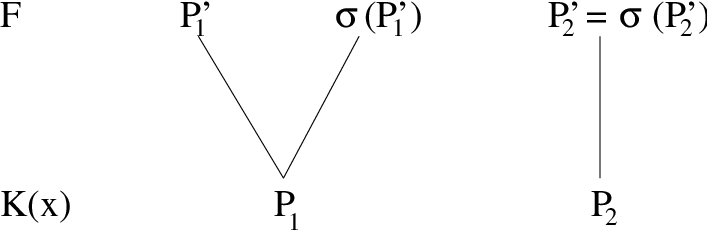
Every hyperelliptic curve respectively hyperelliptic function field has an bijective map $\sigma$ of order two called conjugation, flipping the two places lying over one place $P$ of $K(x)$ , if $P$ splits, otherwise the one place lying over $P$ is mapped to itself.

Proof.

If there are two places $P_{1},\,P_{2}\in\mathbb{P}_{F}$ lying over $P\in\mathbb{P}_{K(x)}$ , Theorem 3.46 states that there exists an isomorphism $\sigma$ with $\sigma(P_{1})=P_{2}$ respectively $\sigma(P_{2})=P_{1}$ , because there are only two places lying over $P$ . Therefore $\sigma(\sigma(P_{1}))=\sigma(P_{2})=P_{1}$ and $\sigma$ is of order 2. If there is just one place $P^{\prime}|P$ , we have $\sigma(P^{\prime})=P^{\prime}$ , because elements of $K(x)$ are invariant under $\sigma$ . ∎

Figure 3.3 shows that hyperelliptic curves are symmetric. Pictorially, we see that the map $\sigma$ is given by $\sigma(\alpha,\beta)=(\alpha,-\beta)$ . Hence we have that $\sigma(\sigma(\alpha,\beta))=(\alpha,\beta)$ and therefore $\sigma$ is of order two. Figure 3.4 illustrates this.

Example 3.57.

The following Magma [19] calculations show how the rational places split or are ramified. We work over ${K}=\mathbb{F}_{19}$ and use the equation

\displaystyle y^{2}

\displaystyle=

\displaystyle(x-1)(x-2)(x-3)(x-4)(x-5)\in\mathbb{F}_{19}[x,y].

We observe that the second component of each vector is either 0 or there are two vectors with the same first component and the sum of the second components is $0$ .

    F<w> := GF(19);
    P2<x,y,z> := ProjectiveSpace(F,2);
    //Galois field + projective space
    f := 18*y^2*z^3 + (x-z)*(x-2*z)*(x-3*z)*(x-4*z)*(x-5*z);

    X := Curve(P2,f);
    g := Genus(X);
    //construction of a curve X corresponding to f

    > Places(X,1); //rational places of X;
    [
    Place at (0 : 1 : 0),
    Place at (2 : 0 : 1),
    Place at (4 : 0 : 1),
    Place at (16 : 14 : 1),
    Place at (16 : 5 : 1),
    Place at (7 : 13 : 1),
    Place at (7 : 6 : 1),
    Place at (17 : 11 : 1),
    Place at (17 : 8 : 1),
    Place at (15 : 17 : 1),
    Place at (15 : 2 : 1),
    Place at (11 : 12 : 1),
    Place at (11 : 7 : 1),
    Place at (3 : 0 : 1),
    Place at (6 : 14 : 1),
    Place at (6 : 5 : 1),
    Place at (12 : 13 : 1),
    Place at (12 : 6 : 1),
    Place at (5 : 0 : 1),
    Place at (1 : 0 : 1)
    ]

In this list Place at $(x:y:z)$ means the point in ${\mathbb{P}}^{2}$ in homogeneous coordinates. Hence the point $(0:1:0)$ defines the place at infinity.

3.3 Goppa Codes

3.3.1 Standard Goppa Codes

This section gives the basic ideas of Goppa codes. The definitions and theorems are taken from [24], [30], and [29]. In the following, let $\mathbb{F}_{q}$ be a finite field with $q=p^{m}$ , let $p$ be a prime number, and let $F/\mathbb{F}_{q}$ be an algebraic function field.

Definition 3.58.

Let $F/\mathbb{F}_{q}$ be an algebraic function field in one variable. Let $P_{1},\ldots,P_{n}$ be places of degree one and let $D=P_{1}+\cdots+P_{n}$ . Furthermore let $G$ be a divisor with ${\rm supp}(G)\cap{\rm supp}(D)=\emptyset$ . Then the Goppa code (respectively AG code) $C_{\cal L}\subseteq\mathbb{F}_{q}^{n}$ is defined by

\displaystyle C_{\cal L}(D,G)

\displaystyle=

\displaystyle{\left\{(f(P_{1}),\ldots,f(P_{n}))\;|\;f\in{\cal L}(G)\right\}}\subseteq\mathbb{F}_{q}^{n}

Define the following linear evaluation map

\displaystyle\varphi:

\displaystyle\left\{\begin{array}[]{crl}{\cal L}(G)&\rightarrow&\mathbb{F}_{q}^{n}\\ f&\mapsto&(f(P_{1}),\ldots,f(P_{n})).\end{array}\right.

Then the Goppa Code is given by $C_{\cal L}(D,G)=\varphi({\cal L}(G))$ .

Theorem 3.59 ([30, Thm. II.2.2]).

The code $C_{\cal L}(D,G)$ is a linear $\left[n,\,k,\,d\right]$ code with parameters

	$\displaystyle k$	$\displaystyle=$	$\displaystyle\dim G-\dim(G-D)$
	$\displaystyle d$	$\displaystyle\geq$	$\displaystyle n-\deg G=:d_{des}.$

The parameter $d_{des}$ is called the designed distance of the Goppa code.

Corollary 3.60 ([30, Thm. II.2.3]).

Assume $\deg G<n$ and let $g$ be the genus of $F/\mathbb{F}_{q}$ . Then we have:

1.

$\varphi:{\cal L}(G)\rightarrow C_{\cal L}(D,G)$ is injective and $C_{\cal L}(D,G)$ is an $[n,k,d]$ code with

$\displaystyle k$ $\displaystyle=$ $\displaystyle\dim G\geq\deg G+1-g$

$\displaystyle d$ $\displaystyle\geq$ $\displaystyle n-\deg G.$
2.

If in addition $2g-2<\deg G<n$ , then

$\displaystyle k$ $\displaystyle=$ $\displaystyle\deg G+1-g.$

If $(f_{1},\ldots,f_{k})$ is a basis of ${\cal L}(G)$ , then

\displaystyle M

\displaystyle=

\displaystyle\left(\begin{array}[]{ccc}f_{1}(P_{1})&\cdots&f_{1}(P_{n})\\ \vdots&&\vdots\\ f_{k}(P_{1})&\cdots&f_{k}(P_{n})\\ \end{array}\right)

is a generator matrix for $C_{\cal L}(D,G)$ .

Example 3.61.

This example was created with Magma [19] and uses the curve constructed in Example 3.57. We use only the pairs of rational points. Therefore we will be able to use this example for a quantum code construction.

In the following we give an example of a Goppa code in Magma:

    //Function to construct a finite field and a projective space
    constr_field := function(q)
    local F, P2;
      F<w> := GF(q);
      P2<x,y,z> := ProjectiveSpace(F,2);
    return F, P2;
    end function;

    //Function to construct a curve
    constr_curve := function(P2, f)
    local X, g;
      X := Curve(P2,f);
      g := Genus(X);
    return X,g;
    end function;



    //Example of the construction of a Goppa code
    //Construction of the finite field with 19 elements
    //and the corresponding projective space
    F<w>,P2<x,y,z> := constr_field(19);
    //Definition of a polynomial f
    f := 18*y^2*z^3 + (x-z)*(x-2*z)*(x-3*z)*(x-4*z)*(x-5*z);

    //Construction of the curve X corresponding to f
    X,g := constr_curve(P2,f);
    //Divisor group to X
    DG := DivisorGroup(X);
    //Rational places of X
    place1 := Places(X,1);
    //Function field corresponding to X
    F<a,b> := FunctionField(X);

    //Exclusion of the place at infinity
    //and the non splitting place
    D := Exclude(place1,place1[1]); Exclude(~D,place1[14]);
    //Generation of the divisor of rational places for the code
    D3 := &+[DG!D[i]: i in [3..16]];

    //Divisor G for the generation of codewords is an
    //evaluation at the place at infinity
    G := 7* DG!place1[1];
    C := AlgebraicGeometricCode(D,G);

This construction leads to the following code:

    > C;
    [14, 6] Linear Code over GF(19)
    Generator matrix:
    [ 1  0  0  0  0 13  0 14 15 11 17 15  4 16]
    [ 0  1  0  0  0  6  0  5  6 10 13 15 13  1]
    [ 0  0  1  0  0 10  0  7 12 11  2  6  6 14]
    [ 0  0  0  1  0  9  0 12  4  5 16 12  2 13]
    [ 0  0  0  0  1  1  0  0  4  4  5  5  3  3]
    [ 0  0  0  0  0  0  1  1 17 17  5  5 11 11]

Remark 3.62.

To characterize the dual code of a Goppa code we need to look at the original definitions of Goppa by means of differential forms and its relations to the code defined above.

Definition 3.63.

Let $D=P_{1}+\cdots+P_{n}$ be a divisor, where the $P_{i}$ ’s are places of degree one of an algebraic function field $F/\mathbb{F}_{q}$ , Furthermore let $G$ be a divisor with $supp(G)\cap supp(D)=\emptyset$ . Then we define the code $C_{\Omega}(D,G)$ by

\displaystyle C_{\Omega}(D,G)

\displaystyle:=

\displaystyle{\left\{(\mathrm{res}_{P_{1}}\left(\omega\right),\ldots,\mathrm{res}_{P_{n}}\left(\omega\right))\;|\;\omega\in\Omega_{F}(G-D)\right\}}\subseteq\mathbb{F}_{q}^{n}.

Proposition 3.64 ([29, Thm. 2.4 and 2.5]).

The code $C_{\Omega}(D,G)$ , where $D$ and $G$ are as above has the following properties:

1.

$C_{\cal L}(D,G)^{\perp}=C_{\Omega}(D,G)$ .
2.

$C_{\Omega}(D,G)=a\cdot C_{\cal L}(D,H)$ with $H=D-G+(\eta)$ where $\eta$ is a differential, $v_{P_{i}}(\eta)=-1$ for $i=1,\ldots,n$ , and $a=(\mathrm{res}_{P_{1}}\left(\eta\right),\ldots,\mathrm{res}_{P_{n}}\left(\eta\right))$ .
3.

$C_{\cal L}(D,G)^{\perp}=a\cdot C_{\cal L}(D,H)$ .

The following proposition is cited from [30, Prop. VII.1.2]. It allows to construct differentials with special properties that help to construct a self-orthogonal code.

Proposition 3.65.

Let $x$ and $y$ be elements of $F$ such that $v_{P_{i}}(y)=1$ , $v_{P_{i}}(x)=0$ and $x(P_{i})=1$ for $i=1,\ldots,n$ . Then the differential $\eta:=x\cdot\frac{dy}{y}$ satisfies $v_{P_{i}}(\eta)=-1$ and $\mathrm{res}_{P_{i}}\left(\eta\right)=1$ for $i=1,\ldots,n$ .

3.3.2 Weighted Self-Orthogonal Goppa Codes

Chapter 2 shows that quantum codes have to satisfy certain self-orthogonality properties. In order to find codes satisfying them, we will have to work with some codes which are what we call “weighted self-orthogonal”.

Definition 3.66.

We call a Goppa code weighted self-orthogonal if it satisfies

\displaystyle C

\displaystyle\subseteq

\displaystyle C^{\perp^{a}}

with respect to the inner product

\displaystyle\langle x,y\rangle^{a}

\displaystyle:=

\displaystyle\sum_{i=1}^{n}a_{i}\;x_{i}\,y_{i},

where $a=(a_{i})^{n}\in\mathbb{F}_{q}^{n}$ .

Corollary 3.67.

$\langle x,y\rangle^{a}:=\sum_{i=1}^{n}a_{i}\;x_{i}\,y_{i}$ defines an inner product over $\mathbb{F}_{q}^{n}$ .

Proof.

We have to show bilinearity and symmetry to proof this corollary. Bilinearity is shown in the following.

$\displaystyle\langle\lambda x+z,y\rangle^{a}$	$\displaystyle=$	$\displaystyle\sum_{i=1}^{n}a_{i}\;(\lambda x_{i}+z_{i})\,y_{i}$
	$\displaystyle=$	$\displaystyle\lambda\sum_{i=1}^{n}a_{i}\;x_{i}\,y_{i}+\sum_{i=1}^{n}a_{i}\;z_{i}\,y_{i}$
	$\displaystyle=$	$\displaystyle\lambda\langle x,y\rangle^{a}+\langle z,y\rangle^{a},$

for $\lambda\in\mathbb{F}_{q}$ and $x,y,z\in\mathbb{F}_{q}^{n}$ . Symmetry is given by

$\displaystyle\langle x,y\rangle^{a}$	$\displaystyle=$	$\displaystyle\sum_{i=1}^{n}a_{i}\;x_{i}\,y_{i}$
	$\displaystyle=$	$\displaystyle\sum_{i=1}^{n}a_{i}\;y_{i}\,x_{i}$
	$\displaystyle=$	$\displaystyle\langle y,x\rangle^{a}.$

∎

Corollary 3.68.

Similarly, $\langle x,y\rangle_{s}^{a}=\sum_{i=1}^{n}a_{i}\;(x_{i}y_{n+i}-x_{n+i}y_{i})$ defines a symplectic inner product over $\mathbb{F}_{q}^{2n}$ .

Proof.

We have to show that $\langle x,y\rangle_{s}^{a}$ is bilinear, anti-symmetric and that every vector is self-orthogonal. First we show bilinearity in the following.

$\displaystyle\langle\lambda x+z,y\rangle_{s}^{a}$	$\displaystyle=$	$\displaystyle\sum_{i=1}^{n}a_{i}\;((\lambda x_{i}+z_{i})y_{n+i}-(\lambda x_{n+i}+z_{n+i})\,y_{i})$
	$\displaystyle=$	$\displaystyle\lambda\sum_{i=1}^{n}a_{i}\;(x_{i}y_{n+i}-x_{n+i}y_{i})+\sum_{i=1}^{n}a_{i}\;(z_{i}y_{n+i}-z_{n+i}y_{i})$
	$\displaystyle=$	$\displaystyle\lambda\langle x,y\rangle_{s}^{a}+\langle z,y\rangle_{s}^{a}$

for $\lambda\in\mathbb{F}_{q}$ and $x,y,z\in\mathbb{F}_{q}^{2n}$ . The form is anti-symmetric:

$\displaystyle\langle x,y\rangle_{s}^{a}$	$\displaystyle=$	$\displaystyle\sum_{i=1}^{n}a_{i}\;(x_{i}y_{n+i}-x_{n+i}y_{i})$
	$\displaystyle=$	$\displaystyle-\sum_{i=1}^{n}a_{i}\;(y_{i}x_{n+i}-y_{n+i}x_{i})$
	$\displaystyle=$	$\displaystyle-\langle y,x\rangle_{s}^{a}.$

And every vector has length zero:

$\displaystyle\langle x,x\rangle_{s}^{a}$	$\displaystyle=$	$\displaystyle\sum_{i=1}^{n}a_{i}\;(x_{i}x_{n+i}-x_{n+i}x_{i})$
	$\displaystyle=$	$\displaystyle\sum_{i=1}^{n}a_{i}\;(x_{i}x_{n+i}-x_{i}x_{n+i})$
	$\displaystyle=$	$\displaystyle 0.$

∎

This concludes the chapter about basics in algebraic geometry in which we have established a sufficient background to construct quantum codes over algebraic curves.

Chapter 4 Good Binary Quantum Goppa Codes

In this chapter we give a detailed account of R. Matsumoto’s paper “Algebraic geometric construction of a quantum stabilizer code” [20] and an explicit description of his code construction.

Throughout this chapter let $\mathbb{F}_{q}$ be a finite field with $q=p^{m}$ for some prime number $p$ . In the explicit construction of a code we use a binary field, i.e. $q=2^{m}$ , but most of the theorems also hold for non-binary fields and can be used in Chapter 5. Therefore we state them in the more general case.

4.1 Existence and Decoding of Quantum Codes

First, we show under which circumstances a quantum stabilizer code can be obtained from an algebraic geometric construction. Subsequently we present a method how decoding and error correction can be implemented for these codes.

4.1.1 Existence and Encoding

Proposition 4.1.

Let $F/\mathbb{F}_{q}$ be an algebraic function field of one variable, $\sigma$ an automorphism of order 2 of $F$ which leaves $\mathbb{F}_{q}$ invariant, and $P_{1},\ldots,P_{n}$ pairwise distinct places of degree one such that $\sigma P_{i}\neq P_{j},\;\forall\,i,j=1,\dots,n$ . Let $\eta$ be a differential with the following properties:

\left\{\begin{array}[]{l}v_{P_{i}}(\eta)=v_{\sigma P_{i}}(\eta)=-1,\\ res_{P_{i}}(\eta)=1,\\ res_{\sigma P_{i}}(\eta)=-1.\end{array}\right.

(4.1)

The existence of such $\eta$ is guaranteed by the strong approximation theorem of discrete valuations (see Theorem 3.27). Further assume that we have a divisor $G$ such that $\sigma G=G$ , $v_{P_{i}}(G)=v_{\sigma P_{i}}(G)=0$ for all $i$ . Define

\displaystyle C(G)

\displaystyle=

\displaystyle{\left\{(f(P_{1}),\ldots,f(P_{n}),f(\sigma P_{1}),\ldots,f(\sigma P_{n}))\;|\;f\in{\cal{L}}(G)\right\}}\subseteq\mathbb{F}_{q}^{2n}.

Let

\displaystyle H

\displaystyle=

\displaystyle(P_{1}+\cdots+P_{n}+\sigma P_{1}+\cdots+\sigma P_{n})-G+(\eta),

where $\eta$ is as in Equation (4.1). Then we have $C(G)^{\perp_{s}}=C(H)$

Proof.

Let $x=(x_{1},\ldots,x_{2n})\in\mathbb{F}_{q}^{2n}$ and $y=(y_{1},\ldots,y_{2n})\in\mathbb{F}_{q}^{2n}$ .

(i)

Note that $\sigma(\sigma(f))=f$ , because $\sigma$ is of order 2.
(ii)

Let ${\cal L}^{\sigma}(G):={\left\{\sigma(x)\in F\;|\;(x)\geq-G\right\}}\cup{\left\{0\right\}}$ . As $\sigma G=G$ , we get for $f\in{\cal L}(G)$ :

$\sigma(f)\in{\cal L}^{\sigma}(G)$

so

$\displaystyle\sigma(f)\in{\cal L}(\sigma G)$ $\displaystyle=$ $\displaystyle{\cal L}(G).$

(iii)

This gives us for $(x_{1},\ldots,x_{2n})\in C(G)$

\begin{array}[]{cl}&(x_{1},\ldots,x_{2n})\in C(G)\\ \Longleftrightarrow&\exists\;f\in{\cal L}(G)\hbox{ with }\\ &(x_{1},\ldots,x_{2n})=(f(P_{1}),\ldots,f(P_{n}),f(\sigma P_{1}),\ldots,f(\sigma P_{n}))\in C(G).\end{array}

Remark (ii) gives the equivalence to

\displaystyle(\sigma(f)(P_{1}),\ldots,\sigma(f)(P_{n}),\sigma(f)(\sigma P_{1}),\ldots,\sigma(f)(\sigma P_{n}))\in C(G).

With [30, Prop. VII.3.3] we can rewrite this expression as

\displaystyle(f(\sigma P_{1}),\ldots,f(\sigma P_{n}),f(\sigma\sigma P_{1}),\ldots,f(\sigma\sigma P_{n}))\in C(G).

Finally Remark (i) gives equivalence to

			$\displaystyle(f(\sigma P_{1}),\ldots,f(\sigma P_{n}),f(P_{1}),\ldots,f(P_{n}))\in C(G)$
		$\displaystyle\Longleftrightarrow$	$\displaystyle(x_{n+1},\ldots,x_{2n},x_{1},\ldots,x_{n})\in C(G).$

(iv)

With help of this observation, we can show that $C(G)^{\perp_{s}}=C(H)$ :

Let $x\in C(H)$ . Then with Proposition 3.64 we get for all $y\in C(G)$ :

$\displaystyle 0$	$\displaystyle=$	$\displaystyle\sum\limits_{i=1}^{n}res_{P_{i}}(\eta)\;x_{i}y_{i}+\sum\limits_{i=n+1}^{2n}res_{\sigma P_{i}}(\eta)\;x_{i}y_{i}$
	$\displaystyle=$	$\displaystyle\sum\limits_{i=1}^{n}1\cdot x_{i}y_{i}+\sum\limits_{i=n+1}^{2n}(-1)\cdot x_{i}y_{i}$
	$\displaystyle=$	$\displaystyle\sum\limits_{i=1}^{n}x_{i}y_{i}-\sum\limits_{i=n+1}^{2n}x_{i}y_{i}.$

With (iii) this is equivalent to that for all $y\in C(G)$

\displaystyle\sum\limits_{i=1}^{n}x_{i}y_{n+i}-\sum\limits_{i=1}^{n}x_{n+i}y_{i}

\displaystyle=

\displaystyle 0,

and therefore $x\in C(G)^{\perp_{s}}$ .

Hence by choosing an automorphism of order 2 and suitable residues, we can render the identity $C(G)^{\perp}=a\cdot\,C(H)$ , which we know from classical coding theory into the identity $C(G)^{\perp_{s}}=C(H)$ . ∎

This proposition tells us that the orthogonal code of $C(G)$ is generated by $H$ . The following corollary is a result of the combination of Theorem 3.59 and Proposition 4.1 above and gives us the wanted quantum code:

Corollary 4.2.

We use the same notations as in Proposition 4.1. Furthermore, we assume that $G\geq H$ . Then we can construct an $[[n,k,d]]$ quantum code $Q$ , where

\displaystyle k

\displaystyle=

\displaystyle\dim G-\dim(G-P_{1}-\cdots-P_{n}-\sigma P_{1}-\cdots-\sigma P_{n})-n.

For the minimum distance $d$ of $Q$ , we have

\displaystyle d

\displaystyle\geq

\displaystyle n-\left\lfloor\frac{\deg G}{2}\right\rfloor.

Proof.

Theorem 2.36 and Proposition 4.1 show that we can construct a quantum stabilizer code from $C(D,G)$ , because

			$\displaystyle G\geq H$
		$\displaystyle\Leftrightarrow$	$\displaystyle{\cal L}(G)\supseteq{\cal L}(H)$
		$\displaystyle\Leftrightarrow$	$\displaystyle C(D,G)\supseteq C(D,H)=C(D,G)^{\perp_{s}}.$

By Theorem 2.36 we get $k=\dim C(D,G)-n$ . Then Theorem 3.59 implies

\displaystyle\dim C(D,G)

\displaystyle=

\displaystyle\dim G-\dim(G-P_{1}-\cdots-P_{n}-\sigma P_{1}-\cdots-\sigma P_{n})

and the statement for the dimension of the code $k$ is proven.

The next step is to prove the stated bound on the minimum distance $d$ . Suppose that

\displaystyle{\rm wt}((f(P_{1}),\ldots,f(\sigma P_{n})))

\displaystyle=

\displaystyle\delta\neq 0

for $f\in{\cal L}(G)$ . Then there exists a set ${\left\{i_{1},\ldots,i_{n-\delta}\right\}}$ such that

\displaystyle f(P_{i_{1}})=f(\sigma P_{i_{1}})=\cdots=f(P_{i_{n-\delta}})=f(\sigma P_{i_{n-\delta}})=0,

which implies that $f\in{\cal L}(G-\sum_{j=1}^{n-\delta}(P_{i_{j}}+\sigma P_{i_{j}}))$ . Since $f\neq 0$ , we have

			$\displaystyle\dim(G-\sum_{j=1}^{n-\delta}(P_{i_{j}}+\sigma P_{i_{j}}))>0$
		$\displaystyle\stackrel{{\scriptstyle{\rm Cor.\;\ref{degdim}}}}{{\Longrightarrow}}$	$\displaystyle\deg(G-\sum_{j=1}^{n-\delta}(P_{i_{j}}+\sigma P_{i_{j}}))\geq 0$
		$\displaystyle\Longleftrightarrow$	$\displaystyle\deg G-2(n-\delta)\geq 0$
		$\displaystyle\Longleftrightarrow$	$\displaystyle 2\delta\geq 2n-\deg G$
		$\displaystyle\Longleftrightarrow$	$\displaystyle\delta\geq n-\left\lfloor\frac{\deg G}{2}\right\rfloor.$

∎

As in classical AG codes, this construction provides good codes only when $q$ is large. Matsumoto [20] uses the following theorem to construct $q$ -ary quantum codes from $q^{m}$ ones, if $q$ is small:

Theorem 4.3 (Ashikhmin and Knill [1]).

Let $m$ be a positive integer and $\{\alpha_{1},\ldots,\alpha_{m}\}$ an $\mathbb{F}_{q}$ -basis of $\mathbb{F}_{q^{m}}$ . Define $\mathbb{F}_{q}$ -linear maps $\alpha:\mathbb{F}_{q}^{m}\rightarrow\mathbb{F}_{q^{m}}$ sending $(x_{1},\ldots,x_{m})$ to $x_{1}\alpha_{1}+\cdots+x_{m}\alpha_{m}$ , and $\beta:\mathbb{F}_{q}^{m}\rightarrow\mathbb{F}_{q^{m}}$ sending $(x_{1},\ldots,x_{m})$ to

(\alpha_{1},\ldots,\alpha_{m})M\left(\begin{array}[]{c}x_{1}\\ \vdots\\ x_{m}\end{array}\right)\in\mathbb{F}_{q^{m}}

where $M$ is an $m\times m$ matrix defined by $M_{ij}={\rm tr}_{q}^{q^{m}}(\alpha_{i},\alpha_{j})$ , where ${\rm tr}$ denotes the trace map from $\mathbb{F}_{q^{m}}$ onto $\mathbb{F}_{q}$ . For $C\subseteq\mathbb{F}_{q^{m}}^{2n}$ , let

\gamma(C)={\left\{(\alpha^{-1}(x_{1}),\ldots,\alpha^{-1}(x_{n}),\beta^{-1}(x_{n+1}),\ldots,\beta^{-1}(x_{2n}))|(x_{1},\lx@nobreakspace\ldots,x_{2n})\in C\right\}}

$\subseteq\mathbb{F}_{q}^{2mn}$ . If $C^{\perp_{s}}\subseteq C$ for $C\subseteq\mathbb{F}_{q^{m}}^{2n}$ , then $(\gamma(C))^{\perp_{s}}\subseteq\gamma(C)$ . We also have $d(\gamma(C)\backslash(\gamma(C))^{\perp_{s}})\geq d(C\backslash C^{\perp_{s}})$ .

Now, as we have seen the existence of a quantum code from curves, we still need to know how to decode it and correct errors. This is described in the following paragraph:

4.1.2 Decoding and Error Correction

To decode this code, we can use the Algorithm of Farrán [4]. Matsumoto reduced his code to Farrán’s algorithm as follows:

Reduction 4.4.

If there exists a vector $e\in\mathbb{F}_{q}^{2n}$ such that $\langle e,b_{i}\rangle_{s}=s_{i}$ for $i=1,\ldots,n-k$ and that

2{\rm wt}(e)+1\leq n-\left\lfloor\frac{\deg G}{2}\right\rfloor,

(4.2)

where $\{b_{1},\ldots,b_{n-k}\}$ is a basis of $C(G)^{\perp_{s}}=C(H)$ constructed in Corollary 4.2, then we can efficiently find $e$ from $s_{1},\ldots,s_{n-k}$ as follows. The algorithm of Farrán [4] efficiently finds the unique vector $x$ having the minimum Hamming weight ${\rm wt}_{H}(x)$ in the set ${\left\{y\in\mathbb{F}_{q}^{2n}|\langle y,b_{i}\rangle_{s}=s_{i}\;{\rm for}\;i=1,\ldots,n-k\right\}}$ from given $s_{1},\ldots,s_{n-k}$ , provided that $2{\rm wt}_{H}(x)+1\leq 2n-\deg G$ , where $\langle x,b_{i}\rangle$ is the standard inner product of $x$ and $b_{i}$ and ${\left\{b_{1},\ldots,b_{n-k}\right\}}$ is a basis of $C(H)$ in $O(n^{2.81})$ . Let $e=(e_{1},\ldots,e_{2n})$ and $e^{\prime}=(-e_{n+1},\ldots,-e_{2n},e_{1},\ldots,e_{n})$ . Then $s_{i}=\langle e^{\prime},b_{i}\rangle=\langle e,b_{i}\rangle_{s}$ . Since ${\rm wt}_{H}(e^{\prime})\leq 2{\rm wt}(e)$ , Equation (4.2) implies

\displaystyle 2{\rm wt}_{H}(e^{\prime})+1

\displaystyle\leq

\displaystyle 2n-\deg G,

and the algorithm of Farrán finds $e^{\prime}$ from $s_{1},\ldots,s_{n-k}$ correctly. We can easily find $e$ from $e^{\prime}$ with the map

\displaystyle(e_{1},\ldots,e_{n},e_{n+1},\ldots,e_{2n})

\displaystyle\mapsto

\displaystyle(e_{n+1},\ldots,e_{2n},-e_{1},\ldots,-e_{n}).

4.2 Construction and Bounds

This section gives the explicit construction of a quantum stabilizer code over $\mathbb{F}_{2^{m}}$ , its properties, and shows some bounds on the rate $k/n$ and the relative minimum distance $d/n$ .

Proposition 4.5.

For an integer $m\geq 2$ there exists a sequence of binary quantum stabilizer codes with parameters $\left[\left[n_{i},\,k_{i},\,d_{i}\right]\right]$ such that

$\displaystyle\lim\limits_{i\rightarrow\infty}n_{i}$	$\displaystyle=$	$\displaystyle\infty,$
$\displaystyle\liminf\limits_{i\rightarrow\infty}\frac{k_{i}}{n_{i}}$	$\displaystyle\geq$	$\displaystyle R_{m}^{(1)}(\delta),$
$\displaystyle\liminf\limits_{i\rightarrow\infty}\frac{d_{i}}{n_{i}}$	$\displaystyle\geq$	$\displaystyle\delta,$

where

\displaystyle R_{m}^{(1)}(\delta)

\displaystyle=

\displaystyle 1-\frac{2}{2^{m}-1}-4m\delta.

Proof.

The proof is divided into two parts: First we will explicitly construct a tower of algebraic function fields and Goppa codes derived from these fields. Later we will prove that these codes have the claimed properties.

Construction

1.

We use the Garcia-Stichtenoth function field [7]. Its properties and how to construct it is explained in Section 3.1.8. Here we use it in the following way: Let $q=2^{m}$ , let $F_{i}=\mathbb{F}_{q^{2}}(x_{1},z_{2},\ldots,z_{n})$ , $i\geq 2$ and

$\displaystyle z_{i}^{q}+z_{i}-x_{i-1}^{q+1}$ $\displaystyle=$ $\displaystyle 0,$

$\displaystyle x_{i}$ $\displaystyle=$ $\displaystyle\frac{z_{i}}{x_{i-1}}.$
2.

Claim 1 The Galois group of $F_{i}/F_{i-1}$ is isomorphic to the additive group of $\mathbb{F}_{2}^{m}$ and there exists a $\sigma\in{\rm Gal}(F_{i}/F_{i-1})$ of order 2.

Proof. Apply Proposition 3.47 and Proposition 3.48 of Section 3.1.9. Here $[F_{i}:F_{i-1}]=q=2^{m}$ , so we get that ${\rm Gal}(F_{i}/F_{i-1})$ is isomorphic to $(\mathbb{Z}/2\mathbb{Z})^{m}$ which is equal to the additive group of $\mathbb{F}_{2}^{m}$ . The existence of $\sigma$ follows from the fact that in $\mathbb{F}_{2}^{m}$ all elements are self-inverse.
3.

Let $n_{i}:=\frac{(q^{2}-1)q^{i-1}}{2}$ and $y=x_{1}^{q^{2}-1}-1$ .
Claim 2 The zero divisors of $y$ consist of $2n_{i}$ places of degree 1.

Proof. As our field extension satisfies the conditions of Lemma 3.45 of Section 3.1.8, we can apply it. So we get that there are exactly $q^{2}-1$ places $P$ of degree one in $F_{1}$ and $q^{i-1}$ over every $P$ , so all together $(q^{2}-1)\cdot q^{i-1}=2n_{i}$ places of degree one in $F_{i}$ . By construction, all zeros of $y$ are of degree one.
4.

Let $F_{i}^{\sigma}$ be the fixed field of $\sigma$ . Let $Q$ be a zero of $y$ .

Claim 3 There exists a zero $Q^{\prime}$ of $y$ such that $Q^{\prime}\neq Q$ and $Q\cap F_{i}^{\sigma}=Q^{\prime}\cap F_{i}^{\sigma}$ .

Proof. The isomorphism $\sigma$ is an element of the Galois group of order 2. This means that every zero of $y$ is mapped to another one and applying $\sigma$ twice gives the identity. Therefore the zeros come in pairs as shown in the picture below. Hence $\sigma Q=Q^{\prime}$ and $\sigma Q^{\prime}=Q$ . For all $x\in Q\cap F_{i}^{\sigma}$ we have $\sigma(x)=x$ , whence $x\in Q^{\prime}$ and $x\in F_{i}^{\sigma}$ , i.e. $x\in Q^{\prime}\cap F_{i}^{\sigma}$ . The other inclusion can be shown similarly.
5.

Claim 4 Since $F_{i}/F_{i}^{\sigma}$ is Galois, we have that $\sigma Q=Q^{\prime}$ . Therefore we can write the zero divisor of $y$ as

$P_{1}+\sigma P_{1}+\cdots+P_{n_{i}}+\sigma P_{n_{i}}$

such that $\sigma P_{j}\neq P_{\ell}$ for all $1\leq j,\;\ell\leq n_{i}$ .

Proof. The first part is clear by the proof of Claim 3 and Theorem 3.46. With the property that all zeros are conjugated by $\sigma$ , it is clear that one can write the zero divisor of $y$ as claimed.

Let

	$\displaystyle\eta$	$\displaystyle=$	$\displaystyle\frac{dy}{y}\;=\;\frac{dy}{dx_{1}}\;\frac{dx_{1}}{y}\;=\;\frac{d(x_{1}^{q^{2}-1})}{dx_{1}}\;\frac{dx_{1}}{y}$
		$\displaystyle=$	$\displaystyle(q^{2}-1)x_{1}^{q^{2}-2}\;\frac{dx_{1}}{y}.$

As we work over a binary field, we have $q^{2}-1=1$ , therefore

\displaystyle\eta

\displaystyle=

\displaystyle x_{1}^{q^{2}-2}\;\frac{dx_{1}}{y}.

Claim 5 $\eta$ satisfies the conditions of Equation (4.1) in Proposition 4.1 and can be used for our construction.

Proof.

(a)

$v_{P_{i}}(1)=v_{\sigma P_{i}}(1)=0$
(b)

$v_{P_{i}}(y)=v_{\sigma P_{i}}(y)=1$ , because the elements $P_{i}$ and $\sigma P_{i}$ are simple poles of $y=x_{1}^{q^{2}-1}-1$ .
(c)

$1(P_{i})=1(\sigma P_{i})=1$ .

(d)

Now we can apply Proposition 3.65, which leads to

$\displaystyle v_{P_{i}}(\eta)$	$\displaystyle=$	$\displaystyle v_{\sigma P_{i}}(\eta)=-1,$
$\displaystyle\mathrm{res}_{P_{i}}\left(\eta\right)$	$\displaystyle=$	$\displaystyle 1,$
$\displaystyle\mathrm{res}_{\sigma P_{i}}\left(\eta\right)$	$\displaystyle=$	$\displaystyle 1=-1\;\mathrm{since}\;{\rm char}(\mathbb{F}_{q^{2}})=2.$

Hence all conditions are satisfied and we can use $\eta$ to construct codes.

Let $G_{0}^{\prime}:=(\eta)+P_{1}+\sigma P_{1}+\cdots+P_{n_{i}}+\sigma P_{n_{i}}$ , and $P_{\infty}$ the unique pole of $x_{1}$ in $F_{i}$ . (For existence see Section 3.1.8.) Then we can apply Lemma 3.49 and get

$\displaystyle(\eta)$	$\displaystyle=$	$\displaystyle(x_{1}^{q^{2}-2}\;\frac{dx_{1}}{y})$
	$\displaystyle=$	$\displaystyle(x_{1}^{q^{2}-2})+(dx_{1})-(y)$
	$\displaystyle=$	$\displaystyle(q^{2}-2)(x_{1})+(dx_{1})$
		$\displaystyle-(P_{1}+\sigma P_{1}+\cdots+P_{n_{i}}+\sigma P_{n_{i}}+\underbrace{v_{P_{\infty}}(x_{1}^{q^{2}-1})P_{\infty}}_{\mathrm{pole}\;\mathrm{divisor}\;\mathrm{of}\;y})$
	$\displaystyle=$	$\displaystyle(q^{2}-2)(x_{1})+(dx_{1})$
		$\displaystyle-(P_{1}+\sigma P_{1}+\cdots+P_{n_{i}}+\sigma P_{n_{i}}+(q^{2}-1)v_{P_{\infty}}(x_{1})P_{\infty}).$

From this follows that we can write $G_{0}^{\prime}$ as

$\displaystyle G_{0}^{\prime}$	$\displaystyle=$	$\displaystyle(q^{2}-2)(x_{1})+(dx_{1})$
		$\displaystyle-(P_{1}+\sigma P_{1}+\cdots+P_{n_{i}}+\sigma P_{n_{i}}+(q^{2}-1)v_{P_{\infty}}(x_{1})P_{\infty})$
		$\displaystyle+P_{1}+\sigma P_{1}+\cdots+P_{n_{i}}+\sigma P_{n_{i}}$
	$\displaystyle=$	$\displaystyle(q^{2}-2)(x_{1})-(q^{2}-1)v_{P_{\infty}}(x_{1})P_{\infty}+(dx_{1})$

Claim 6 The valuation of the divisor $G_{0}^{\prime}$ is an even integer at every place of $F_{i}$ .
Proof. To show this, we will have a closer look at the individual summands of $G_{0}^{\prime}$ .

(a)

$v_{P_{\infty}}(x_{1})=-q^{i-1}$
By Lemma 3.42 in Section 3.1.8, we know that $v_{P_{\infty}(F_{1})}(x_{1})=-1$ and the unique pole is totally ramified in all extensions. Denote $P_{\infty}$ in $F_{j}$ by $P_{\infty}(F_{j})$ .We get that $e(P_{\infty}(F_{j}))=e(P_{\infty}(F_{j})\,|\,P_{\infty}(F_{j-1}))=q$ for all $j\geq 2$ and therefore

$\displaystyle v_{P_{\infty}(F_{i})}(x_{1})$	$\displaystyle=$	$\displaystyle e(P_{\infty}(F_{i}))\cdot v_{P_{\infty}(F_{i-1})}(x_{1})$
	$\displaystyle=$	$\displaystyle\cdots\,=\,q^{i-1}v_{P_{\infty}(F_{1})}(x_{1})\,=\,q^{i-1}\cdot(-1)$
	$\displaystyle=$	$\displaystyle-\,q^{i-1}$

(b)

The discrete valuation of $(dx_{1})$ is given by

$(dx_{1})=(1)-2(x_{1})_{\infty}+{\rm Diff}(F_{i}/F_{1})$

This follows immediately from Lemma 3.49 in Section 3.1.9.

(c)

The discrete valuation of $(dx_{1})$ is even at every place of $F_{i}$ .
For all $P_{j}\in\{P_{1},\sigma P_{1},\ldots,P_{n_{i}},\sigma P_{n_{i}}\}$

$\displaystyle v_{P_{j}}((dx_{1}))$	$\displaystyle=$	$\displaystyle v_{P_{j}}((1))+v_{P_{j}}(-2(x_{1})_{\infty})+v_{P_{j}}({\rm Diff}(F_{i}/F_{1}))$
	$\displaystyle=$	$\displaystyle 0-2\cdot v_{P_{j}}(P_{\infty})+\sum\limits_{P\in\mathbb{P}_{F_{1}}}\sum\limits_{P^{\prime}\|P}d(P^{\prime}\|P)\cdot v_{P_{j}}(P^{\prime})$
	$\displaystyle=$	$\displaystyle\underbrace{-2\cdot v_{P_{j}}(P_{\infty})}_{\mathrm{even}}+\underbrace{\sum\limits_{P\in\mathbb{P}_{F_{1}}}\sum\limits_{P^{\prime}\|P}\underbrace{d(P^{\prime}\|P)}_{\mathrm{even}}\cdot v_{P_{j}}(P^{\prime})}_{\mathrm{even}}$

The last equation follows because the elements $d(P^{\prime}|P)$ are all even: By Lemma 3.43 in Section 3.1.7, all places of degree one in $F_{i}$ are either totally ramified over $F_{i-1}$ with different exponent $d(P^{\prime})=(q-1)(q+2)$ , or unramified, so $e(P^{\prime})=1$ and $char(\mathbb{F}_{q^{2}})=2\,\not|\;1$ . Therefore we can apply Dedekind’s Different Theorem (see Theorem 3.38) and get $d(P^{\prime})=e(P^{\prime})-1=0$ . As $2\,|\,(q-1)(q+2)$ and $2\,|\,0$ , $d(P^{\prime})$ is also even over $F_{1}$ for all $P^{\prime}$ with $P^{\prime}|P\in\mathbb{P}_{F_{1}}$ .

Hence we conclude

$\displaystyle G_{0}^{\prime}$	$\displaystyle=$	$\displaystyle(q^{2}-2)(x_{1})-(q^{2}-1)v_{P_{\infty}}(x_{1})P_{\infty}+(dx_{1})$
	$\displaystyle=$	$\displaystyle(q^{2}-2)(x_{1})-(q^{2}-1)\underbrace{(-q^{i-1})}_{\mathrm{(a)}}P_{\infty}$
		$\displaystyle+\underbrace{(1)-2(x)_{\infty}+{\rm Diff}(F_{i}/F_{1})}_{\mathrm{(b)}}$
	$\displaystyle=$	$\displaystyle\underbrace{(q^{2}-2)(x_{1})}_{\mathrm{even}}+\underbrace{(q^{2}-1)\underbrace{q^{i-1}}_{\mathrm{even}}}_{\mathrm{even}}P_{\infty}+\underbrace{(1)-2(x)_{\infty}+{\rm Diff}(F_{i}/F_{1})}_{\mathrm{(c)}\;\Rightarrow\;\mathrm{even}}$

and the valuation of $G_{0}^{\prime}$ is even.

With the result of Claim 6, we can define $G_{0}:=\frac{1}{2}G_{0}^{\prime}$ and get

$\displaystyle\deg G_{0}$	$\displaystyle=$	$\displaystyle\frac{1}{2}\deg G_{0}^{\prime}$
	$\displaystyle=$	$\displaystyle\frac{1}{2}((q^{2}-2)\underbrace{\deg(x_{1})}_{=\,0\;\mathrm{(a)}}+\underbrace{(q^{2}-1)q^{i-1}}_{=\,2n_{i}}\underbrace{\deg P_{\infty}}_{=\,1}+\deg(dx_{1}))$
	$\displaystyle=$	$\displaystyle\frac{1}{2}(2n_{i}+\deg(dx_{1}))$
	$\displaystyle=$	$\displaystyle\frac{1}{2}(2n_{i}+\underbrace{2g_{i}-2}_{\mathrm{(b)}})$
	$\displaystyle=$	$\displaystyle n_{i}+g_{i}-1$

where $g_{i}$ is the genus of $F_{i}/\mathbb{F}_{q^{2}}$ .

(a)

$(x_{1})$ is a principal divisor and therefore it has degree zero.
(b)

$(dx_{1})$ is a canonical divisor and therefore it has degree $2g_{i}-2$ .

10.

Let $j$ be a nonnegative integer.
Claim 7 $G_{0}+jP_{\infty}$ satisfies the conditions on $G$ in Proposition 4.1.

Proof. We have to show that $\sigma(G_{0}+jP_{\infty})=G_{0}+jP_{\infty}$ . Denote that poles are mapped to poles and zeros are mapped to zeros under $\sigma$ and $P_{\infty}$ is unique.

$\displaystyle\sigma(G_{0}+jP_{\infty})$	$\displaystyle=$	$\displaystyle\sigma G_{0}+j\sigma P_{\infty}\;=\;\sigma G_{0}+jP_{\infty}$	(4.3)
	$\displaystyle=$	$\displaystyle\sigma\left(\frac{1}{2}\left((q^{2}-2)(x_{1})-(q^{2}-1)q^{i-1}P_{\infty}+(dx_{1})\right)\right)$
		$\displaystyle+jP_{\infty}$
	$\displaystyle=$	$\displaystyle\frac{q^{2}-2}{2}\;\sigma\left(\sum_{P}v_{P}(x_{1})P\right)-\frac{(q^{2}-1)q^{i-1}}{2}\sigma P_{\infty}$
		$\displaystyle+\sigma\left(\sum_{P}v_{P}(dx_{1})P\right)+jP_{\infty}$
	$\displaystyle=$	$\displaystyle\frac{q^{2}-2}{2}\sigma\left(\sum_{P\neq P_{\infty},\;\neq P_{x_{1}}}0\cdot P+1\cdot P_{x_{1}}+(-1)P_{\infty}\right)$
		$\displaystyle-\frac{(q^{2}-1)q^{i-1}}{2}P_{\infty}$
		$\displaystyle+\sigma\left(\sum_{P\neq P_{\infty}}v_{P}(1)P+v_{P_{\infty}}(dx_{1})P_{\infty}\right)+jP_{\infty}$
	$\displaystyle=$	$\displaystyle\frac{q^{2}-2}{2}(P_{x_{1}}-P_{\infty})-\frac{(q^{2}-1)q^{i-1}}{2}P_{\infty}-2P_{\infty}+jP_{\infty}$
	$\displaystyle=$	$\displaystyle\frac{q^{2}-2}{2}\;\sum_{P}v_{P}(x_{1})P-\frac{(q^{2}-1)q^{i-1}}{2}P_{\infty}$
		$\displaystyle+\sum_{P}v_{P}(dx_{1})P+jP_{\infty}$
	$\displaystyle=$	$\displaystyle\frac{1}{2}((q^{2}-2)(x_{1})-(q^{2}-1)q^{i-1}P_{\infty}+(dx_{1}))+jP_{\infty}$
	$\displaystyle=$	$\displaystyle G_{0}+jP_{\infty}$

Equation (4.3) follows because of the following: Let us have a look at the properties of $dx_{1}$ . Denote that $x_{1}$ is a $P$ -prime element for all $P$ except $P_{\infty}$ . For $P_{\infty}$ we can use $\frac{1}{x_{1}}$ as $P$ -prime element. Therefore for $P\neq P_{\infty}$

\displaystyle v_{P}(dx_{1})

\displaystyle=

\displaystyle v_{P}(1\cdot dx_{1})\stackrel{{\scriptstyle\mathrm{Def.}}}{{=}}v_{P}(1).

For $P=P_{\infty}$ we get

\displaystyle dx_{1}

\displaystyle=

\displaystyle\frac{dx_{1}}{d\frac{1}{x_{1}}}\;d\frac{1}{x_{1}}=-\left(\frac{1}{x_{1}}\right)^{-2}\;d\frac{1}{x_{1}}

which implies that

v_{P_{\infty}}(dx_{1})=v_{P_{\infty}}\left(-\left(\frac{1}{x_{1}}\right)^{-2}d\frac{1}{x_{1}}\right)=v_{P_{\infty}}\left(-\left(\frac{1}{x_{1}}\right)^{-2}\right)=-2

11.

Let

$\displaystyle H$	$\displaystyle=$	$\displaystyle(P_{1}+\cdots+P_{n_{i}}+\sigma P_{1}+\cdots+\sigma P_{n_{i}})-(G_{0}+jP_{\infty})+(\eta)$
	$\displaystyle=$	$\displaystyle(P_{1}+\cdots+P_{n_{i}}+\sigma P_{1}+\cdots+\sigma P_{n_{i}})$
		$\displaystyle-\left(\frac{1}{2}((\eta)+P_{1}+\sigma P_{1}+\cdots+P_{n_{i}}+\sigma P_{n_{i}})+jP_{\infty}\right)+(\eta)$
	$\displaystyle=$	$\displaystyle\frac{1}{2}\left((\eta)+P_{1}+\sigma P_{1}+\cdots+P_{n_{i}}+\sigma P_{n_{i}}\right)-jP_{\infty}$
	$\displaystyle=$	$\displaystyle G_{0}-jP_{\infty}.$

Then $G_{0}+jP_{\infty}\geq G_{0}-jP_{\infty}=H$ , and therefore by Proposition 4.1

	$\displaystyle C(G_{0}+jP_{\infty})^{\perp_{s}}$	$\displaystyle=$	$\displaystyle C(H)\;=\;C(G_{0}-jP_{\infty})$
		$\displaystyle\subseteq$	$\displaystyle C(G_{0}+jP_{\infty}).$

By Corollary 4.2, we can construct a quantum stabilizer code from $C$ .

Properties of the Constructed Code

Claim 8 By Corollary 4.2 for $i,j\in{\mathbb{N}}$ we can construct an $[[n_{i},k_{ij},d_{ij}]]$ stabilizer code with

k_{ij}\geq j,\;d_{ij}\geq(n_{i}-g_{i}-j+1)/2

Proof. Corollary 4.2 implies that

\begin{array}[]{cclcl}d_{ij}&\geq&n_{i}-\left\lfloor\frac{\deg G}{2}\right\rfloor\par&=&n_{i}-\overbrace{\left\lfloor\frac{\deg G_{0}+jP_{\infty}}{2}\right\rfloor}^{\geq 0}\\ &\stackrel{{\scriptstyle\mathrm{(9.)}\;\mathrm{constr.}}}{{=}}&n_{i}-\left\lfloor\frac{n_{i}+g_{i}-1+j}{2}\right\rfloor&\geq&n_{i}-\frac{n_{i}+g_{i}-1+j}{2}\\ &=&\frac{n_{i}-g_{i}-j+1}{2}.\end{array}

For $k_{ij}$ we have to assume $j\leq n_{i}-g_{i}$ and obtain then

$\displaystyle k_{ij}$	$\displaystyle=$	$\displaystyle\dim G$	(4.4)
		$\displaystyle-\dim(G-P_{1}-\cdots-P_{n_{i}}-\sigma P_{1}-\cdots-\sigma P_{n_{i}})-n_{i}$
	$\displaystyle=$	$\displaystyle\dim(G_{0}+jP_{\infty})-\dim(-G_{0}+jP_{\infty}+(\eta))-n_{i}$
	$\displaystyle\geq$	$\displaystyle\deg(G_{0}+jP_{\infty})+1-g_{i}-\dim(-G_{0}+jP_{\infty}+(\eta))-n_{i}$
	$\displaystyle=$	$\displaystyle[(n_{i}+g_{i}-1)+j+(1-g_{i})-n_{i}]$
		$\displaystyle-\dim(-G_{0}+jP_{\infty}+(\eta))$	(4.5)
	$\displaystyle=$	$\displaystyle j$	(4.6)

In these calculations, Equation (4.4) follows from Theorem 3.26, Equation (4.5) follows from 9. of the code construction and Equation(4.6) is a consequence of the following calculations:

$\displaystyle\deg(-G_{0}+jP_{\infty}+(\eta))$	$\displaystyle=$	$\displaystyle-(n_{i}+g_{i}-1)+j+(2g_{i}-2)$
	$\displaystyle=$	$\displaystyle g_{i}-n_{i}-1+j$
	$\displaystyle\leq$	$\displaystyle g_{i}-n_{i}-1+(n_{i}-g_{i})$
	$\displaystyle=$	$\displaystyle-1$
	$\displaystyle<$	$\displaystyle 0$

By Corollary 3.25 it follows immediately that $\dim(-G_{0}+jP_{\infty}+(\eta))=0$ .

Let $R$ be a real number such that $0\leq R\leq 1$ and $\lfloor Rn_{i}\rfloor\leq n_{i}-g_{i}$ . Set $j:=\lfloor Rn_{i}\rfloor$ . By Theorem 4.3 we can construct a sequence of $[[n_{i},k_{i},d_{i}]]$ binary quantum stabilizer codes.

Claim 9 This code has the following properties

\displaystyle\liminf\limits_{i\rightarrow\infty}\frac{k_{i}}{n_{i}}

\displaystyle\geq

\displaystyle R_{m}^{(1)}(\delta),\qquad\liminf\limits_{i\rightarrow\infty}\frac{d_{i}}{n_{i}}\quad\geq\quad\delta,

where

\displaystyle R_{m}^{(1)}(\delta)

\displaystyle=

\displaystyle 1-\frac{2}{2^{m}-1}-4m\delta.

Proof.

\displaystyle\liminf\limits_{i\rightarrow\infty}\frac{k_{i}}{n_{i}}

\displaystyle\geq

\displaystyle\liminf\limits_{i\rightarrow\infty}\frac{j_{i}}{n_{i}}\quad=\quad\liminf\limits_{i\rightarrow\infty}\frac{\lfloor Rn_{i}\rfloor}{n_{i}}\quad=\quad R

The binary code obtained from Theorem 4.3 has rate $\frac{2m\cdot k_{i}}{2m\cdot n_{i}}=\frac{k_{i}}{n_{i}}$ and therefore the same rate as the higher dimensional case. Moreover,

$\displaystyle\liminf\limits_{i\rightarrow\infty}\frac{d_{i}}{n_{i}}$	$\displaystyle\geq$	$\displaystyle\liminf\limits_{i\rightarrow\infty}\frac{(n_{i}-g_{i}-j_{i}+1)/2}{n_{i}}$	(4.7)
	$\displaystyle=$	$\displaystyle\frac{1}{2}\liminf\limits_{i\rightarrow\infty}\frac{n_{i}-g_{i}-\lfloor Rn_{i}\rfloor+1}{n_{i}}$
	$\displaystyle=$	$\displaystyle\frac{1-R-2/(2^{m}-1)}{2}$
	$\displaystyle\geq$	$\displaystyle\frac{1-R-2/(2^{m}-1)}{4m}=:\delta$

And for the binary case

	$\displaystyle\liminf\limits_{i\rightarrow\infty}\frac{d_{i}}{2m\cdot n_{i}}$	$\displaystyle\geq$	$\displaystyle\liminf\limits_{i\rightarrow\infty}\frac{(n_{i}-g_{i}-j_{i}+1)/2}{2m\cdot n_{i}}$
		$\displaystyle=$	$\displaystyle\frac{1-R-2/(2^{m}-1)}{4m}=:\delta.$

Equation (4.7) follows if we use the genus formula of Theorem 3.44 and calculate

•

For $i=1\;{\rm mod}\;2$ :

$\displaystyle\lim\limits_{i\rightarrow\infty}\frac{n_{i}}{g_{i}}$	$\displaystyle=$	$\displaystyle\lim\limits_{i\rightarrow\infty}\frac{(2^{2m}-1)(2^{m})^{i-1}/2}{(2^{m})^{i}+(2^{m})^{i-1}-(2^{m})^{\frac{i-1}{2}}+1}$
	$\displaystyle=$	$\displaystyle\frac{1}{2}\frac{2^{2m}-1}{2^{m}+1}$
	$\displaystyle=$	$\displaystyle\frac{1}{2}\frac{(2^{m}+1)(2^{m}-1)}{2^{m}+1}$
	$\displaystyle=$	$\displaystyle\frac{2^{m}-1}{2}.$

•

and for $i=0\;{\rm mod}\;2$ :

\begin{array}[]{l}\lim\limits_{i\rightarrow\infty}\frac{n_{i}}{g_{i}}\\ \begin{array}[]{ll}=&\lim\limits_{i\rightarrow\infty}\frac{(2^{2m}-1)(2^{m})^{i-1}/2}{(2^{m})^{i}+(2^{m})^{i-1}-\frac{1}{2}(2^{m})^{\frac{i}{2}+1}-\frac{3}{2}(2^{m})^{\frac{i}{2}}-(2^{m})^{\frac{i}{2}-1}+1}\\ =&\frac{1}{2}\frac{2^{2m}-1}{2^{m}+1}\\ =&\frac{1}{2}\frac{(2^{m}+1)(2^{m}-1)}{2^{m}+1}\\ =&\frac{2^{m}-1}{2}.\end{array}\end{array}

We now can calculate $R_{m}^{(1)}(\delta)=R$ :

\begin{array}[]{cccc}&\delta&=&\frac{1-R-2/(2^{m}-1)}{4m}\\ \Longleftrightarrow&4m\delta&=&1-R-2/(2^{m}-1)\\ \Longleftrightarrow&R&=&1-\frac{2}{2^{m}-1}-4m\delta,\end{array}

which establishes the claimed result.

∎

4.3 A Small Example for the Construction

Next, we give an example for a code we get from Matsumoto’s construction. To do so, we consider the shortest possible length. Let $m=2$ and $i=2$ , so $q=2^{2}=4$ and therefore we use the field $\mathbb{F}_{4^{2}}=\mathbb{F}_{16}$ . Then $F_{1}=\mathbb{F}_{16}(x_{1})$ is the rational function field and $F_{2}=F_{1}(z_{2})=\mathbb{F}_{16}(x_{1},z_{2})$ with

\displaystyle z_{2}^{4}+z_{2}-x_{1}^{5}

\displaystyle=

\displaystyle 0.

Using Magma [19] we can calculate the genus of the extension:

Magma V2.11-5
Type ? for help.  Type <Ctrl>-D to quit.
> F<w> := GF(16);
> P2<x,y,z> := ProjectiveSpace(F,2);
> f := y^4*z + y*z^4 - x^5;
> X := Curve(P2, f);
> g := Genus (X);
> g;
6

Now we are able to estimate $k$ and $d$ :

\displaystyle k_{2,j}\geq j,\qquad d_{2,j}\geq\frac{n_{2}-g_{2}-j+1}{2}

\displaystyle=

\displaystyle\frac{30-6-j+1}{2}=12-\frac{j-1}{2}

This gives us the possibility to choose a suitable value for $R$ . We will have a look at two examples.

Set $R=\frac{1}{2}$ , then $j=\frac{1}{2}\cdot 30=15$ . We get

k_{2,15}\geq 15,\qquad d_{2,15}\geq 12-\frac{15-1}{2}=5.

Using Theorem 4.3, we get for the parameters of the binary code

n=4\cdot n_{2}=120,\qquad k=4\cdot k_{2,15}\geq 60,\qquad d=d_{2,15}\geq 5.

Therefore we can calculate the ratios

\frac{k}{n}\geq\frac{60}{120}=\frac{1}{2},\qquad\frac{d}{n}\geq\frac{5}{120}=\frac{1}{24}

and the limits are bounded by

\liminf\limits_{i\rightarrow\infty}\frac{k_{i}}{n_{i}}\geq\frac{1}{2},\qquad\liminf\limits_{i\rightarrow\infty}\frac{d_{i}}{n_{i}}\geq\frac{1-\frac{1}{2}-\frac{2}{4-1}}{4\cdot 2}=-\frac{1}{48}.

This gives an estimate $<0$ and therefore is not a valid parameter.

Set $R=\frac{1}{3}$ , then $j=\frac{1}{3}\cdot 30=10$ . This gives us

k_{2,10}\geq 10,\qquad d_{2,10}\geq 12-\frac{10-1}{2}=7.5,\;\mathrm{so}\;d_{2,10}\geq 8.

From Theorem 4.3, we get for the binary code

n=4\cdot n_{2}=120,\qquad k=4\cdot k_{2,10}\geq 40,\qquad d=d_{2,10}\geq 8.

Therefore we can calculate the ratios

\frac{k}{n}\geq\frac{40}{120}=\frac{1}{3},\qquad\frac{d}{n}\geq\frac{8}{120}=\frac{1}{15}

and the limits are bounded by

\liminf\limits_{i\rightarrow\infty}\frac{k_{i}}{n_{i}}\geq\frac{1}{3},\qquad\liminf\limits_{i\rightarrow\infty}\frac{d_{i}}{n_{i}}\geq\frac{1-\frac{1}{3}-\frac{2}{4-1}}{4\cdot 2}=0.

Hence $R=\frac{1}{3}$ is the threshold in order to get $\frac{d}{n}\geq 0$ . Therefore we should use $R\leq\frac{1}{3}$ . This gives an $\left[\left[120,\,\geq 40,\,\geq 8\right]\right]$ binary quantum error correcting code.

Chapter 5 Codes over Hyperelliptic Curves

The following chapter uses the machinery introduced in the preceding chapters to construct quantum error correcting codes from Goppa codes. We will work over fields of odd characteristic. If we would work in characteristic $2$ we would get the first step of the hierarchy used in Matsumoto’s construction explained in the preceding chapter.

In this chapter we will first look at the CSS construction that can be applied to all self-orthogonal AG codes. We will generalise this construction to weighted self-orthogonal codes. Afterwards we will directly construct quantum Goppa codes, comparable to Matsumoto’s construction in [20]. Finally we shall see some examples that illustrate the construction.

5.1 The CSS Construction Revisited

This section shows how we can use hyperelliptic curves to construct quantum AG codes. The construction is similar to the one in the next section, but is easier to prove.

5.1.1 General Construction

1.

Let ${K}:=\mathbb{F}_{p^{m}}$ be a finite field of odd characteristic, and choose a hyperelliptic curve

$\displaystyle y^{2}$ $\displaystyle=$ $\displaystyle f(x),$

where $f(x)$ is a square-free polynomial of degree $\geq 5$ . Let $F:=K(x,y)$ be the corresponding function field. (see Chapter 3)
2.

Then $F$ has a set of rational places (see Definition 3.17). We choose any subset of pairs and denote it by $SP={\left\{P_{1},\ldots,P_{n}\right\}}$ .

Set $D=P_{1}+\cdots+P_{n}$ and $G=(\left\lfloor\frac{n}{2}\right\rfloor+g-1-r)P_{\infty}$ , where $r$ can be chosen with $0\leq r\leq n-g$ and $P_{\infty}$ the place at infinity. We also set $(\eta)=W=-D+(n+2g-2)P_{\infty}$ . Then $W$ is a canonical divisor to the differential

$\displaystyle\eta$ $\displaystyle=$ $\displaystyle\frac{1}{y\;\prod_{P_{i}\,\rm{corr.}\,\alpha_{i}}(x-\alpha_{i})}{\rm d}x.$

Proof.

The proof is similar to the one given in Lemma 5.4. ∎
3.

Denote the residues of $\eta$ at the places $P_{1},\ldots,P_{n}$ by

$a_{i}=\mathrm{res}_{P_{i}}\left(\eta\right).$

for $i=1,\ldots,n$ .
4.

Now we can construct a classical Goppa code $C(D,G)$ (see Section 3.3) with

$C(D,G)^{\perp}=C(D,H)\cdot{\rm diag}(a_{1},\ldots,a_{n})$

where $H=D-G+W$ is defined as usual (proof see Theorem 2.5 in [29]). The code satisfies $C(D,G)\subseteq C(D,H)$ and therefore $C(D,G)\subseteq C(D,G)^{\perp^{a}}$ with respect to the inner product $\langle\;,\,\rangle^{a}$ . This will be shown in Corollary 5.1.
5.

If not all coefficients $a_{i}$ are in the base field, we can transform our code to a code $C^{\prime}(D,G)$ that satisfies $C^{\prime}(D,G)\subseteq C^{\prime}(D,G)^{\perp^{b}}$ with respect to a new inner product $\langle x,y\rangle^{b}=\sum_{i=1}^{n}b_{i}x_{i}y_{i}$ where all $b_{i}$ are in $\mathbb{F}_{p}$ , if $m$ is odd. This is proved in Proposition 5.2.

Now we take two copies of $C^{\prime}(D,G)$ and multiply in the first copy every codeword component wise with the corresponding coefficient $b_{i}$ . Then we can apply the CSS construction and get a generator matrix

\displaystyle{\cal G}

\displaystyle=

\displaystyle\left(\begin{array}[]{ccc|ccc}{b_{1}\cdot c_{1,1}}&\cdots&{b_{n}\cdot c_{1,n}}&0&\cdots&0\\ \vdots&\ddots&\vdots&\vdots&\ddots&\vdots\\ {b_{1}\cdot c_{l,1}}&\cdots&{b_{n}\cdot c_{l,n}}&0&\cdots&0\\ 0&\cdots&0&{c_{1,1}}&\cdots&{c_{1,n}}\\ \vdots&\ddots&\vdots&\vdots&\ddots&\vdots\\ 0&\cdots&0&{c_{l,1}}&\cdots&{c_{l,n}}\end{array}\right),

if the classical code $C^{\prime}(D,G)$ has generator matrix

\left(\begin{array}[]{ccc}c_{1,1}&\cdots&{c_{1,n}}\\ \vdots&\ddots&\vdots\\ {c_{l,1}}&\cdots&{c_{l,n}}\\ \end{array}\right).

A proof of this is given in Corollary 5.3.

7.

If we want to project this code and used the modifications of the original code above, we can apply the special case where all coefficients $a_{i}$ are in the base field $\mathbb{F}_{p}$ . Therefore this CSS construction has a nice down projection that allows us to write the new code as a symmetric one with weights $a_{i}$ in the $X$ component.

5.1.2 Correctness of the Construction

To justify and clarify the above construction, in the following subsection we prove all statements claimed in the last section.

Corollary 5.1.

Let $C(D,G)$ be the Goppa code constructed in Section 5.1.1 with $G=(\left\lfloor\frac{n}{2}\right\rfloor+g-1-r)P_{\infty}$ and

a=(a_{1},\ldots,a_{n})=(\mathrm{res}_{P_{1}}\left(\eta\right),\ldots,\mathrm{res}_{P_{n}}\left(\eta\right)).

Then the code satisfies $C(D,G)\subseteq C(D,H)$ with $H=D-G+(\eta)$ and therefore

C(D,G)\subseteq C(D,G)^{\perp^{a}}

with respect to the inner product $\langle\;,\,\rangle^{a}$ .

Proof.

First we have to calculate $H$ :

$\displaystyle H$	$\displaystyle=$	$\displaystyle D-G+(\eta)$
	$\displaystyle=$	$\displaystyle D-\left(\left\lfloor\frac{n}{2}\right\rfloor+g-1-r\right)P_{\infty}+(-D+(n+2g-2)P_{\infty})$
	$\displaystyle=$	$\displaystyle\left(\left\lceil\frac{n}{2}\right\rceil+g-1+r\right)P_{\infty}$
	$\displaystyle\geq$	$\displaystyle G.$

Therefore $C(D,G)\subseteq C(D,H)$ and by [29, Thm. 2.5]

\displaystyle C(D,G)^{\perp}

\displaystyle=

\displaystyle C(D,H)\cdot{\rm diag}(a_{1},\ldots,a_{n}).

It follows that all codewords $x,y$ of $C(D,G)$ satisfy

\displaystyle\sum_{i=1}^{n}a_{i}\,x_{i}y_{i}

\displaystyle=

\displaystyle 0,

and $C(D,G)$ is self orthogonal with respect to the inner product

\displaystyle\langle x,y\rangle^{a}

\displaystyle=

\displaystyle\sum_{i=1}^{n}a_{i}\,x_{i}y_{i}.

∎

Proposition 5.2.

If not all weights $a_{i}$ are in the base field, we can transform our code to a code $C^{\prime}(D,G)$ that satisfies $C^{\prime}(D,G)\subseteq C^{\prime}(D,G)^{\perp^{b}}$ with respect to a new inner product $\langle x,y\rangle^{b}=\sum_{i=1}^{n}b_{i}x_{i}y_{i}$ where all $b_{i}$ are in $\mathbb{F}_{p}$ , if $m$ is odd.

Proof.

The idea is to use Stichtenoth’s proof how to transform residue squares into residues with value one (Corollary 3.4 in [29]).

1.

For all elements that satisfy $\mathrm{res}_{P_{i}}\left(\eta\right)=b_{i}^{2}$ for some $b_{i}\in\mathbb{F}_{p^{m}}$ , set $u(P_{i})=b_{i}$ . For all the others with $\mathrm{res}_{P_{i}}\left(\eta\right)=d_{i}$ and $d_{i}$ is not a square, set $u(P_{i})=1$ . The existence of u is given by the Strong Approximation Theorem (see Theorem 3.27). Set $G^{\prime}=G-(u)$ with new residues $\mathrm{res}_{P_{i}}\left(u^{-2}\eta\right)=\mathrm{res}_{P_{i}}\left(\eta^{\prime}\right)=1$ for all elements that were squares. The residues of the other $P_{i}$ stay $d_{i}$ .

The residues for our new code over $G^{\prime}$ are 1 if possible. All elements of $\mathbb{F}_{p^{m}}$ are of the form $\alpha^{r}$ with $r=1,\ldots,p^{m}$ and $\alpha$ a generator of $\mathbb{F}_{p^{m}}$ . The idea is to transform all residues to elements of the base field. It turns out that this is only possible under the circumstances that $m$ is odd. We get this result from the following calculations: The elements of the base field are those which satisfy the equation

\beta^{p-1}=1=\beta^{p^{m}-1}

We can use this property to find elements $b_{i}$ satisfying

(b_{i}^{-2}\alpha^{r_{i}})^{p-1}=1=\alpha^{p^{m}-1},

where $\alpha^{r_{i}}=d_{i}$ . Denote $b_{i}:=\alpha^{k_{i}}$ for some $k_{i}$ . Our goal is to find $k_{i}$ that satisfies the equation above. We have that

$\displaystyle(b_{i}^{-2}\alpha^{r_{i}})^{p-1}$	$\displaystyle=$	$\displaystyle\alpha^{p^{m}-1},$
$\displaystyle\alpha^{(-2k_{i}+r_{i})(p-1)}$	$\displaystyle=$	$\displaystyle\alpha^{p^{m}-1},$
$\displaystyle(r_{i}-2k_{i})(p-1)$	$\displaystyle=$	$\displaystyle c\cdot(p^{m}-1),$

for some $c$ (because of ${\rm mod}\;p^{m}-1$ ). We know that

\displaystyle s:=(p^{m}-1)/(p-1)

\displaystyle=

\displaystyle p^{m-1}+\cdots+1

and $s$ is odd iff $m$ is odd. Our equation can be transformed to $2k_{i}=r_{i}-c\cdot s$ . As the elements $r_{i}$ are odd (otherwise they are squares which would have been transformed to 1 in step 1), $c\cdot s$ has to be odd. Therefore $s$ has to be odd and this yields that $m$ odd. Hence $r_{i}-c\cdot s$ is even and we can divide it by 2. Therefore we can find $k_{i}$ such that our equation $2k_{i}=r_{i}-c\cdot s$ is satisfied and our residues can be transformed by

\displaystyle k_{i}

\displaystyle=

\displaystyle\frac{r_{i}-c\cdot s}{2}

to elements of $\mathbb{F}_{p}\ {\left\{0\right\}}$ . Therefore we get a code $C^{\prime}(D,G)$ that is self-orthogonal with respect to an inner product with weights (residues) $b_{i}$ in $\mathbb{F}_{p}$ . We can apply the trace operation on the code and the inner product over $\mathbb{F}_{p^{m}}$ and get the weights out of the trace:

$\displaystyle{\rm tr}(\langle x,y\rangle^{b})$	$\displaystyle=$	$\displaystyle\sum_{i=1}^{n}{\rm tr}(b_{i}\;x_{i}y_{i})$
	$\displaystyle=$	$\displaystyle\sum_{i=1}^{n}{\rm tr}(b_{i}\sum_{j=1}^{m}\sum_{k=1}^{m}x_{i}^{(j)}y_{i}^{(k)}\alpha_{j}\alpha_{k})$
	$\displaystyle=$	$\displaystyle\sum_{i=1}^{n}\sum_{k=1}^{m}\sum_{l=1}^{m}b_{i}\;x_{i}^{(j)}y_{i}^{(k)}\underbrace{{\rm tr}(\alpha_{j}\alpha_{k})}_{\delta_{jk}}$

where $\{\alpha_{1},\ldots,\alpha_{m}\}$ is a self-dual basis for $\mathbb{F}_{p^{m}}/\mathbb{F}_{p}$ , i.e. for all basis elements holds ${\rm tr}(\alpha_{i}\alpha_{j})=\delta_{ij}$ (for existence see [17, Ch. 2, Notes 3.]) and

\displaystyle x_{i}

\displaystyle=

\displaystyle x_{i}^{(1)}\alpha_{1}+\cdots+x_{i}^{(m)}\alpha_{m}

for all codewords $x$ . Therefore we get a code over $\mathbb{F}_{p}$ that stays self-orthogonal with respect to an inner product $\langle\;,\;\rangle^{b}$ .

∎

Corollary 5.3.

Take two copies of $C^{\prime}(D,G)$ defined above and multiply in the first copy every codeword component wise with the coefficients $b_{i}$ . Then we can apply the CSS construction and get a generator matrix

\displaystyle{\cal G}

\displaystyle=

\displaystyle\left(\begin{array}[]{ccc|ccc}{b_{1}\cdot c_{1,1}}&\cdots&{b_{n}\cdot c_{1,n}}&0&\cdots&0\\ \vdots&\ddots&\vdots&\vdots&\ddots&\vdots\\ {b_{1}\cdot c_{l,1}}&\cdots&{b_{n}\cdot c_{l,n}}&0&\cdots&0\\ 0&\cdots&0&{c_{1,1}}&\cdots&{c_{1,n}}\\ \vdots&\ddots&\vdots&\vdots&\ddots&\vdots\\ 0&\cdots&0&{c_{l,1}}&\cdots&{c_{l,n}}\end{array}\right)

if the classical code $C^{\prime}(D,G)$ has generator matrix

{\cal G}_{cl}=\left(\begin{array}[]{ccc}c_{1,1}&\cdots&{c_{1,n}}\\ \vdots&\ddots&\vdots\\ {c_{l,1}}&\cdots&{c_{l,n}}\\ \end{array}\right).

Proof.

The classical code $C^{\prime}(D,G)$ satisfies

\displaystyle\langle x,y\rangle^{b}

\displaystyle=

\displaystyle 0

for all codewords $x,y$ . So if ${\cal G}_{cl}$ is a generator matrix of the classical code

\displaystyle{\cal G}

\displaystyle=

\displaystyle\left(\begin{array}[]{c|c}{\cal G}_{cl}&0\\ 0&{\cal G}_{cl}\end{array}\right)

is a valid CSS quantum stabilizer code with respect to the symplectic inner product

\displaystyle\langle x,y\rangle_{s}^{b}

\displaystyle=

\displaystyle\sum_{i=1}^{n}b_{i}\,(x_{i}y_{n+i}-x_{n+i}y_{i}),

because

$\displaystyle\langle(x_{1},\ldots,x_{n},0,\ldots),(y_{1},\ldots,y_{n},0,\ldots)\rangle_{s}^{b}$	$\displaystyle=$	$\displaystyle\sum_{i=1}^{n}b_{i}(x_{i}\cdot 0-0\cdot y_{i})=0,$
$\displaystyle\langle(0,\ldots,x_{n+1},\ldots,x_{2n}),(0,\ldots,y_{n+1},\ldots,y_{2n})\rangle_{s}^{b}$	$\displaystyle=$	$\displaystyle\sum_{i=1}^{n}b_{i}(0\cdot y_{n+i}-x_{n+i}\cdot 0)$
	$\displaystyle=$	$\displaystyle 0,$
$\displaystyle\langle(x_{1},\ldots,x_{n},0,\ldots),(0,\ldots,y_{n+1},\ldots,y_{2n})\rangle_{s}^{b}$	$\displaystyle=$	$\displaystyle\sum_{i=1}^{n}b_{i}\,(x_{i}y_{n+i}-0\cdot 0)$
	$\displaystyle=$	$\displaystyle\sum_{i=1}^{n}b_{i}\,x_{i}y_{n+i}=0.$

Now we can apply Lemma 2.32 and transform our CSS code to a quantum code with respect to the standard symplectic inner product. ∎

5.2 Direct Construction and Code Properties

The goal of this section is to show how it is possible to use Goppa codes over hyperelliptic curves to construct quantum stabilizer codes.

5.2.1 Construction of Weighted Self-Orthogonal Codes

In order to make the construction more transparent, we will divide it into several smaller steps. The construction is similar to the one given in Section 5.1.1. First we will present the construction; the corresponding proofs can be found in the following subsections.

1.

see 1. in Construction 5.1.1.
2.

Then $F$ has a set of splitting rational places (see 3.17). Choose a set of pairs

$\displaystyle SP$ $\displaystyle=$ $\displaystyle{\left\{P_{1},\ldots,P_{n},\sigma P_{1},\ldots,\sigma P_{n}\right\}},$

where $\sigma$ denotes the hyperelliptic conjugation and $P_{i}$ and $\sigma P_{i}$ are the two places lying over one rational place in $K(x)$ .

The following elements are similar to Construction 5.1.1, but the values are a bit different because we use $2n$ rational places. Set

$\displaystyle D$ $\displaystyle=$ $\displaystyle P_{1}+\cdots+P_{n}+\sigma P_{1}+\cdots+\sigma P_{n}$

and

$\displaystyle G$ $\displaystyle=$ $\displaystyle(n+g-1-r)P_{\infty}$

where $0\leq r\leq n-g$ can be chosen and $P_{\infty}$ is the place at infinity.

We also set

$\displaystyle(\eta)$ $\displaystyle=$ $\displaystyle W=-D+(2n+2g-2)P_{\infty}.$

Then $W$ is a canonical divisor.

Proof.

$W=(\eta)$ for

$\displaystyle\eta$ $\displaystyle=$ $\displaystyle\frac{1}{y\;\prod_{P_{i}\,\rm{cor.}\,\alpha_{i}}(x-\alpha_{i})}{\rm d}x$

is proved in Lemma 5.4. Therefore $W$ comes from a differential and is canonical. ∎
3.

The residues of $\eta$ at the places $P_{1},\ldots,P_{n},\sigma P_{1},\ldots,\sigma P_{n}$ satisfy

$a_{i}=\mathrm{res}_{P_{i}}\left(\eta\right)=-\mathrm{res}_{\sigma P_{i}}\left(\eta\right).$

for $i=1,\ldots,n$ (proof see Lemma 5.5).
4.

Now we can construct a Goppa code $C(D,G)$ (see Section 3.3) with

$C(D,G)^{\perp_{s}}=C(D,H)\cdot{\rm diag}(a_{1},\ldots,a_{n},1,\ldots,1)$

where $H=D-G+W$ is defined as usual (proof see Proposition 5.6). The code satisfies $C(D,G)\subseteq C(D,H)$ and therefore $C(D,G)\subseteq C(D,G)^{\perp_{s}^{a}}$ with respect to the symplectic inner product $\langle\;,\,\rangle_{s}^{a}$ what is proved in Corollary 5.7.
5.

With the help of Corollary 5.8 we transform $C(D,G)$ to a self-orthogonal code $C^{\prime}(D,G)$ with respect to the standard symplectic inner product by multiplying each component $x_{i}$ of every codeword by the corresponding $a_{i}$ , for $1\leq i\leq n$ . The difference to Construction 5.1.1 is that we have self-orthogonality with respect to a symplectic inner product and not with respect to an inner product.
6.

$C^{\prime}(D,G)$ defines a stabilizer code with parameters $\left[\left[n,\,k,\,d\right]\right]$ , where $n$ is the number of used splitting rational places of the rational function field, $k\geq r$ and $d\geq\frac{n-g+1-r}{2}$ (see Proposition 5.9).

The following subsections include the proofs for the construction above.

The Canonical Divisor and its Residue Properties

In the following construction of a weighted self-orthogonal Goppa code we always set

\displaystyle W

\displaystyle=

\displaystyle-D+(2n+(2g-2))P_{\infty}

where $W$ is the canonical divisor.

Lemma 5.4.

$\eta$ is the differential corresponding to $W$ with

\displaystyle\eta

\displaystyle=

\displaystyle\frac{1}{y\;\prod_{P_{i}\,\rm{cor.}\,\alpha_{i}}(x-\alpha_{i})}{\rm d}x

where the elements $\alpha_{i}$ are the $x$ -coordinates of the points on the curve corresponding to the places $P_{i}$ .

Proof.

We will calculate $(\eta)$ explicitly.

$\displaystyle(\eta)$	$\displaystyle=$	$\displaystyle\left(\frac{1}{y}\right)+\left(\frac{1}{\prod(x-\alpha_{i})}\right)+\left({\rm d}x\right)$	(5.4)
	$\displaystyle=$	$\displaystyle\left(\frac{1}{y}\right)+2nP_{\infty}-\sum P_{i}-\sum\sigma P_{i}-2(x)_{\infty}+{\rm Diff}(F/K(x))$
	$\displaystyle=$	$\displaystyle-\sum_{{\rm irred.\,of}\,f(x)}Q_{i}+(2g+1)P_{\infty}+2nP_{\infty}-\sum P_{i}-\sum\sigma P_{i}$
		$\displaystyle-2\cdot 2P_{\infty}+\sum_{P}\sum_{P^{\prime}\|P}(e(P)-1)P^{\prime}$
	$\displaystyle=$	$\displaystyle-D+(2n+2g-3)P_{\infty}-\sum Q_{i}+\sum 1\cdot Q_{i}+1\cdot P_{\infty}$
	$\displaystyle=$	$\displaystyle-D+(2n+(2g-2))P_{\infty}$
	$\displaystyle=$	$\displaystyle W$	(5.5)

Equation (5.4) follows from that fact that

\displaystyle g=\frac{\deg f(x)-1}{2}

\displaystyle\Longleftrightarrow

\displaystyle\deg f(x)=2g+1

for $(2g+1)P_{\infty}$ , and that $e(P)=2$ for the irreducible components of $f(x)$ and $P_{\infty}$ , otherwise $e(P)=1$ .

∎

Lemma 5.5.

The differential

\displaystyle\eta

\displaystyle=

\displaystyle\frac{1}{y\;\prod_{P_{i}\,\rm{cor.}\,\alpha_{i}}(x-\alpha_{i})}{\rm d}x

satisfies

\displaystyle\mathrm{res}_{P_{i}}\left(\eta\right)

\displaystyle=

\displaystyle-\mathrm{res}_{\sigma P_{i}}\left(\eta\right).

Proof.

Let $(\alpha_{i},\beta_{i})$ be the corresponding point to $P_{i}$ . Then $(\alpha_{i},-\beta_{i})$ is the corresponding to $\sigma P_{i}$ . We get

$\displaystyle\mathrm{res}_{P_{i}}\left(\eta\right)$	$\displaystyle=$	$\displaystyle\frac{1}{\beta_{i}\prod_{i\neq j}(\alpha_{i}-\alpha_{j})}$
$\displaystyle\mathrm{res}_{\sigma P_{i}}\left(\eta\right)$	$\displaystyle=$	$\displaystyle\frac{1}{-\beta_{i}\prod_{i\neq j}(\alpha_{i}-\alpha_{j})}$
	$\displaystyle=$	$\displaystyle-\frac{1}{\beta_{i}\prod_{i\neq j}(\alpha_{i}-\alpha_{j})}$
	$\displaystyle=$	$\displaystyle-\mathrm{res}_{P_{i}}\left(\eta\right).$

∎

Weighted Self-Orthogonality and Quantum Code Construction

The following proposition is similar to Proposition 4.1 except that the residues at the conjugate places do not have to be $1$ and $-1$ , but negative to each other. Proposition 4.1 is stronger, because it shows the existence of a special differential $\eta$ , but the proof is not constructive. Here we prove the weaker version, because the differential constructed in Lemma 5.4 and Lemma 5.5 satisfies these conditions.

Proposition 5.6.

Let $F/\mathbb{F}_{q}$ be an algebraic function field, $\sigma$ an automorphism of order 2 of $F$ not moving elements in $\mathbb{F}_{q}$ , and $P_{1},\ldots,P_{n}$ pairwise distinct places of degree one such that $\sigma P_{i}\neq P_{j}$ for all $i,j=1,\ldots,n$ , $D=P_{1}+\cdots+P_{n}+\sigma P_{1}+\cdots+\sigma P_{n}$ . Let $\eta$ be a differential with the properties

\left\{\begin{array}[]{rcl}v_{P_{i}}(\eta)&=&v_{\sigma P_{i}}(\eta)=-1,\\ \mathrm{res}_{P_{i}}\left(\eta\right)&=&-\mathrm{res}_{\sigma P_{i}}\left(\eta\right).\end{array}\right.

Further assume that we have a divisor $G$ such that $\sigma G=G$ , $v_{P_{i}}(G)=v_{\sigma P_{i}}(G)=0$ . Define

\displaystyle C(D,G)

\displaystyle=

\displaystyle{\left\{(f(P_{1}),\ldots,f(P_{n}),f(\sigma P_{1}),\ldots,f(\sigma P_{n}))\;|\;f\in{\cal L}(G)\right\}}\subseteq\mathbb{F}_{q}^{2n}.

Let $H=D-G+(\eta)$ , then we have $C(D,G)^{\perp_{s}^{a}}=C(D,H)$ where $a=(a_{1},\ldots,a_{n})$ are the weights of the symplectic inner product.

Proof.

The proof is similar to the one of Proposition 4.1. The only difference is the more general assumption that $\mathrm{res}_{P_{i}}\left(\eta\right)=-\mathrm{res}_{\sigma P_{i}}\left(\eta\right)$ , instead of $1$ and $-1$ . ∎

Corollary 5.7.

Let $C(D,G)$ be the Goppa code constructed above and

a=(a_{1},\ldots,a_{n})=(\mathrm{res}_{P_{1}}\left(\eta\right),\ldots,\mathrm{res}_{P_{n}}\left(\eta\right)).

Then the code satisfies $C(D,G)\subseteq C(D,H)$ with $H=D-G+(\eta)$ and therefore

C(D,G)\subseteq C(D,G)^{\perp_{s}^{a}}

with respect to the symplectic inner product $\langle\;,\,\rangle_{s}^{a}$ .

Proof.

Note that $G=(n+g-1-r)P_{\infty}$ and $(\eta)=-D+(2n+2g-2)P_{\infty}$ . Therefore we can calculate $H$ in the following

$\displaystyle H$	$\displaystyle=$	$\displaystyle D-G+(\eta)$
	$\displaystyle=$	$\displaystyle D-(n+g-1-r)P_{\infty}+(-D+(2n+2g-2)P_{\infty})$
	$\displaystyle=$	$\displaystyle(n+g-1+r)P_{\infty}$
	$\displaystyle\geq$	$\displaystyle G.$

So we get ${\cal L}(G)\subseteq{\cal L}(H)$ and thereby $C(D,G)\subseteq C(D,H)$ . Now we apply Proposition 5.6 and use that $C(D,G)^{\perp_{s}^{a}}=C(D,H)$ . This leads to the following implications and concludes the proof:

1.

Then for all $x\in C(D,G)$ , $y\in C(D,H)$ we have that

$\displaystyle\langle x,y\rangle_{s}^{a}$ $\displaystyle=$ $\displaystyle\sum_{i=1}^{n}a_{i}(x_{i}y_{n+i}-x_{n+i}y_{i})=0.$
2.

In particular because $C(D,G)\subseteq C(D,H)$ this equation holds for all $x,y\in C(D,G)$ .
3.

Therefore $C(D,G)\subseteq C(D,G)^{\perp_{s}^{a}}$ and the claim is proved.

∎

Corollary 5.8.

For $G\leq H$ , $G$ and $H$ as above, we have $C(D,G)\subseteq C(D,H)$ . If we multiply

\displaystyle C^{\prime}(D,G)

\displaystyle=

\displaystyle C(D,G)\cdot{\rm diag}(\mathrm{res}_{P_{1}}\left(\eta\right),\ldots,\mathrm{res}_{P_{n}}\left(\eta\right),1,\ldots,1)

then $C^{\prime}$ is a linear self-orthogonal code with respect to the standard symplectic inner product. This code modification does not change the code properties and defines a quantum code.

Proof.

The proof of Corollary 5.7 is independent of the choice of $D$ and $G$ . Therefore $C(D,G)\subseteq C(D,G)^{\perp_{s}^{a}}$ holds under the more general assumptions of this corollary. Hence $C(D,G)$ meets the conditions of a stabilizer code and Lemma 2.32 proves the corollary. ∎

Code Properties

Proposition 5.9.

Let $C^{\prime}(D,G)$ be the Goppa code constructed by Corollary 5.7 and Corollary 5.8. Then $C^{\prime}(D,G)$ is a stabilizer code with parameters $[[n,k,d]]$ where $n$ is the number of used splitting rational places of the rational function field, $k\geq r$ and $d\geq\frac{n-g+1-r}{2}$ .

Proof.

1.

We can construct a stabilizer code, because $C^{\prime}(D,G)\subseteq C^{\prime}(D,G)^{\perp_{s}}$ (see Theorem 2.36). Since our code transformation did not change the code properties we can calculate the properties of $C(D,G)$ in order to get those of $C^{\prime}(D,G)$ .
2.

Now we can apply Corollary 4.2 by changing $G$ and $H$ which enables us to calculate $k$ and $d$ .

For $d$ we get

$\displaystyle d$	$\displaystyle\geq$	$\displaystyle n-\left\lfloor\frac{\deg H}{2}\right\rfloor$
	$\displaystyle=$	$\displaystyle n-\left\lfloor\frac{n+g-1+r}{2}\right\rfloor$
	$\displaystyle\geq$	$\displaystyle\frac{n-g+1-r}{2}.$

For the bound on $k$ we need the Theorem of Riemann-Roch 3.26.

$\displaystyle k$	$\displaystyle=$	$\displaystyle\dim H-\dim(H-D)-n$	(5.6)
	$\displaystyle\geq$	$\displaystyle\deg H+1-g-\dim(H-D)-n$
	$\displaystyle=$	$\displaystyle(n+g-1+r)+1-g-\dim(H-D)-n$
	$\displaystyle=$	$\displaystyle r.$

Equation (5.6) follows because $\dim(H-D)=0$

Proof. Note that $0\leq r\leq n-g$ . Therefore the following equation holds:

$\displaystyle\deg(H-D)$	$\displaystyle=$	$\displaystyle\deg H-\deg D$
	$\displaystyle=$	$\displaystyle(n+g-1+r)-2n$
	$\displaystyle=$	$\displaystyle r-(n-g)-1$
	$\displaystyle\leq$	$\displaystyle-1.$

Now we can apply Corollary 3.25 and get $\dim(H-D)=0$ .

∎

5.3 Projection onto the Prime Field

If we have a code over a field $\mathbb{F}_{p^{m}}$ , it may be desirable to project it onto the base field $\mathbb{F}_{p}$ . For this projection we can use the ideas of Ashikhmin and Knill in [1]. Note that this projection is always possible. In the following we will also see under which circumstances it is possible to find a nicer projection that allows us to see the coefficients $a_{i}$ respectively the new coefficients $a_{ij}$ as weights of the symplectic inner product.

5.3.1 General Case

The general case uses almost completely Ashikhmin and Knill’s ideas in [1]. It gives us the following projection properties.

Proposition 5.10.

Let ${\left\{\alpha_{1},\ldots,\alpha_{m}\right\}}$ be a self-dual basis for $\mathbb{F}_{p^{m}}$ over $\mathbb{F}_{p}$ , then the projection

\displaystyle(a_{1}x_{1},\ldots,a_{n}x_{n},x_{n+1},\ldots,x_{2n})

\displaystyle\mapsto

\displaystyle((a_{1}x_{1})^{(1)},(a_{1}x_{1})^{(2)},\ldots,x_{2n}^{(m)}),

where each component $x_{i}=x_{i}^{(1)}\alpha_{1}+\cdots+x_{i}^{(m)}\alpha_{m}$ is represented in the self-dual basis, of the code $C^{\prime}(D,G)$ onto the base field gives a stabilizer code ${\cal C}(D,G)$ with respect to the symplectic inner product

\displaystyle\langle x,y\rangle_{s}^{p}

\displaystyle=

\displaystyle\sum_{i=1}^{n}\sum_{j=1}^{m}((a_{i}\,x_{i})^{(j)}\,y_{n+i}^{(j)}-x_{n+i}^{(j)}\,(a_{i}\,y_{i})^{(j)}).

Proof.

First observe that if a symplectic inner product of two vectors is zero, then so is the trace over it [1] where the trace of an element $\alpha\in\mathbb{F}_{p^{m}}$ over the base field is defined as

\displaystyle{\rm tr}(\alpha)

\displaystyle=

\displaystyle\sum_{\nu=1}^{m}\sigma_{\nu}\,\alpha,

where the elements $\sigma_{i}$ are the Galois automorphisms of $\mathbb{F}_{p^{m}}/\mathbb{F}_{p}$ [16, Chapter VI.5]. Next we will show that the new code is still self-orthogonal with respect to the new inner product. For $x,y\in C^{\prime}(D,G)$ we get that

$\displaystyle 0={\rm tr}(\langle x,y\rangle_{s})$	$\displaystyle=$	$\displaystyle{\rm tr}\left(\sum_{i=1}^{n}(a_{i}\,x_{i}\,y_{n+i}-x_{n+i}\,a_{i}\,y_{i})\right)$
	$\displaystyle=$	$\displaystyle\sum_{i=1}^{n}\sum_{j=1}^{m}\sum_{k=1}^{m}((a_{i}\,x_{i})^{(j)}\,y_{n+i}^{(k)}-x_{n+i}^{(j)}\,(a_{i}\,y_{i})^{(k)})\underbrace{{\rm tr}(\alpha_{j}\alpha_{k})}_{=\delta_{jk}}$
	$\displaystyle=$	$\displaystyle\sum_{i=1}^{n}\sum_{j=1}^{m}((a_{i}\,x_{i})^{(j)}\,y_{n+i}^{(j)}-x_{n+i}^{(j)}\,(a_{i}\,y_{i})^{(j)}),$

and therefore ${\cal C}(D,G)\subseteq{\cal C}(D,G)^{\perp_{s}^{p}}$ . Finally, we have to show that this code is again a linear code. Therefore let

	$\displaystyle{\cal X}$	$\displaystyle=$	$\displaystyle((a_{1}x_{1})^{(1)},(a_{1}x_{1})^{(2)},\ldots,x_{2n}^{(m)})\;\mathrm{and}$
	$\displaystyle{\cal Y}$	$\displaystyle=$	$\displaystyle((a_{1}y_{1})^{(1)},(a_{1}y_{1})^{(2)},\ldots,y_{2n}^{(m)})\in{\cal C}(D,G),$

then there exist $x,y\in C^{\prime}(D,G)$ with

	$\displaystyle x$	$\displaystyle=$	$\displaystyle((a_{1}x_{1})^{(1)}\alpha_{1}+\cdots+(a_{1}x_{1})^{(m)}\alpha_{m},\ldots,x_{2n}^{(1)}\alpha_{1}+x_{2n}^{(m)}\alpha_{m})$
	$\displaystyle y$	$\displaystyle=$	$\displaystyle((a_{1}y_{1})^{(1)}\alpha_{1}+\cdots+(a_{1}y_{1})^{(m)}\alpha_{m},\ldots,x_{2n}^{(1)}\alpha_{1}+x_{2n}^{(m)}\alpha_{m}).$

Let $s\in\mathbb{F}_{p}$ . As $C^{\prime}(D,G)$ is a linear code, and $\mathbb{F}_{p^{m}}$ is a $\mathbb{F}_{p}$ -linear vector space,

	$\displaystyle s\cdot x+y=([s\cdot(a_{1}x_{1})^{(1)}+(a_{1}y_{1})^{(1)}]\alpha_{1}+\cdots+$
	$\displaystyle[s\cdot(a_{1}x_{1})^{(m)}+(a_{1}y_{1})^{(m)}]\alpha_{m},\ldots,[s\cdot x_{2n}^{(1)}+y_{2n}^{(1)}]\alpha_{1}+[s\cdot x_{2n}^{(m)}+y_{2n}^{(m)}]\alpha_{m})$

is in $C^{\prime}(D,G)$ and therefore

	$\displaystyle s\cdot{\cal X}+{\cal Y}$	$\displaystyle=$	$\displaystyle(s\cdot(a_{1}x_{1})^{(1)}+(a_{1}y_{1})^{(1)},\ldots,s\cdot(a_{1}x_{1})^{(m)}+(a_{1}y_{1})^{(m)},$
			$\displaystyle\ldots,s\cdot x_{2n}^{(1)}+y_{2n}^{(1)},\ldots,s\cdot x_{2n}^{(m)}+y_{2n}^{(m)})\in{\cal C}(D,G).$

Therefore the projected code is a linear code satisfying the symplectic inner product and defines a quantum stabilizer code. ∎

Figure 5.1 illustrates how the codewords split with respect to the self-dual basis. Note that this $p$ -ary linear code cannot necessarily be written as a code of the form

{\cal C}^{\prime}(D,G)\cdot{\rm diag}(a_{1}^{(1)},\ldots,a_{n}^{(m)},1,\ldots,1)

like in the $p^{m}$ -ary case. This is possible in some special cases shown in the next section.

5.3.2 Special Case: The Weights $a_{i}\in\mathbb{F}_{p}$ for all $i$

The following special case allows us to write our projected code in the form

{\cal C}^{\prime}(D,G)\cdot{\rm diag}(a_{1}^{(1)},\ldots,a_{n}^{(m)},1,\ldots,1).

A way to get an easy projection is the case that all $a_{i}$ are elements of $\mathbb{F}_{p}$ , because the trace is $\mathbb{F}_{p}$ -linear, i.e. ${\rm tr}(a_{i})=a_{i}{\rm tr}(1)$ . So we get for all codewords

$\displaystyle 0={\rm tr}{\langle x,y\rangle_{s}^{a}}$	$\displaystyle=$	$\displaystyle{\rm tr}(\sum_{i=1}^{n}a_{i}(x_{i}y_{n+i}-x_{n+i}y_{i}))$
	$\displaystyle=$	$\displaystyle{\rm tr}(\sum_{i=1}^{n}a_{i}\sum_{j=1}^{m}\sum_{k=1}^{m}(x_{i}^{(j)}y_{n+i}^{(k)}\alpha_{j}\alpha_{k}-x_{n+i}^{(j)}y_{i}^{(j)}\alpha_{j}\alpha_{k}))$
	$\displaystyle=$	$\displaystyle\sum_{i=1}^{n}a_{i}\sum_{j=1}^{m}\sum_{k=1}^{m}(x_{i}^{(j)}y_{n+i}^{(k)}-x_{n+i}^{(j)}y_{i}^{(j)})\underbrace{{\rm tr}(\alpha_{j}\alpha_{k})}_{=\delta_{jk}}$
	$\displaystyle=$	$\displaystyle\sum_{i=1}^{n}\sum_{j=1}^{m}a_{i}(x_{i}^{(j)}y_{n+i}^{(k)}-x_{n+i}^{(j)}y_{i}^{(j)}),$

and our new code can be written as

C^{\prime}={\left\{(a_{1}x_{1}^{(1)},\ldots,a_{n}x_{n}^{(m)}|z_{1}^{(1)},\ldots,z_{n}^{(m)})\;:\;(a_{1}x_{1},\ldots,a_{n}x_{n}|z_{1},\ldots,z_{n})\in C\right\}}.

Figure 5.2 shows how the coefficients $a_{i}$ split with respect to the self-dual basis. The figure is just slightly different from the general case of the previous section.

5.4 Examples

5.4.1 Curves with Many Rational Points

An example of a curve with many rational points is given in [28, Theorem 6.14]. We will analyse the case over $\mathbb{F}_{p^{m}}$ where $m$ is odd. Let $y^{2}=f(x)$ with

\displaystyle f(x)

\displaystyle=

\displaystyle(x+x^{p^{\frac{m-1}{2}}})(x+x^{p^{\frac{m+1}{2}}})\qquad\in\mathbb{F}_{p^{m}}[x]

be a hyperelliptic curve. This curve does not satisfy the standard definition of a hyperelliptic curve because it is not square-free, i.e. $x^{2}$ can be extracted from the equation. In the following we see that it is still possible to construct a quantum code, i.e. a quantum code with good parameters.

Claim 5.11.

$f(x)$ has no linear divisors except for $x$ .

Proof.

We can rewrite $f(x)$ as

\displaystyle f(x)

\displaystyle=

\displaystyle x^{2}(1+x^{p^{\frac{m-1}{2}}-1})(1+x^{p^{\frac{m+1}{2}}-1}).

It suffices to show that none of the two factors different from $x^{2}$ is divisible by a linear polynomial.

Let $\alpha\in\mathbb{F}_{p^{m}}$ , then

\displaystyle\frac{1+x^{p^{\frac{m-1}{2}}-1}}{x-\alpha}

\displaystyle=

\displaystyle\sum_{i=0}^{p^{\frac{m-1}{2}}-2}\alpha^{i}x^{p^{\frac{m-1}{2}}-2-i}+\frac{\alpha^{p^{\frac{m-1}{2}}-1}+1}{x-\alpha}.

This equation can only hold if $\alpha^{p^{\frac{m-1}{2}}-1}+1=0$ and therefore $\alpha^{p^{\frac{m-1}{2}}-1}=-1$ . Then $\alpha^{2(p^{\frac{m-1}{2}}-1)}=1$ . This is only possible if $2(p^{\frac{m-1}{2}}-1)|p^{m}-1$ . Assume $2(p^{\frac{m-1}{2}}-1)|p^{m}-1$ , then

\displaystyle\frac{p^{m}-1}{2(p^{\frac{m-1}{2}}-1)}

\displaystyle=

\displaystyle 2^{-1}p^{\frac{m+1}{2}}+2^{-1}p+\frac{p-1}{2(p^{\frac{m-1}{2}}-1)}.

So the assumption is only true if $p-1=0$ , therefore $p=1$ . This contradicts that $p$ is an odd prime greater than two. Therefore we have shown that there exists no linear polynomial dividing $1+x^{p^{\frac{m-1}{2}}-1}$ . Now we have to do the same calculations for the second factor: Let again $\alpha\in\mathbb{F}_{p^{m}}$ , then

\displaystyle\frac{1+x^{p^{\frac{m+1}{2}}-1}}{x-\alpha}

\displaystyle=

\displaystyle\sum_{i=0}^{p^{\frac{m+1}{2}}-2}\alpha^{i}x^{p^{\frac{m-1}{2}}-2-i}+\frac{\alpha^{p^{\frac{m+1}{2}}-1}+1}{x-\alpha}

This equation can only hold if $\alpha^{p^{\frac{m+1}{2}}-1}+1=0$ and therefore $\alpha^{p^{\frac{m+1}{2}}-1}=-1$ . If there exists a solution, then $2(p^{\frac{m+1}{2}}-1)|p^{m}-1$ . Assume this equation is true, then

\displaystyle\frac{p^{m}-1}{2(p^{\frac{m+1}{2}}-1)}

\displaystyle=

\displaystyle 2^{-1}p^{\frac{m-1}{2}}+\frac{p^{\frac{m-1}{2}}-1}{2(p^{\frac{m+1}{2}}-1)}.

So the assumption is only true if $p^{\frac{m-1}{2}}-1=0$ , but the calculations take place in $\mathbb{F}_{p^{m}}$ which is a field of characteristic $p$ and therefore $p^{\frac{m-1}{2}}=0$ which leads to the contradiction $0=-1$ .

We conclude that there exists no $\alpha\neq 0$ such that $x-\alpha$ divides $f(x)$ . Therefore $f(x)$ has no linear divisors except for $x$ . ∎

Corollary 6.15 in [28] shows that it is possible to actually calculate the number of rational points

\displaystyle N_{p^{m}}

\displaystyle=

\displaystyle 2p^{m}-1

As the only linear polynomial that divides $f(x)$ is $x$ , there are $\frac{2p^{m}-4}{2}=p^{m}-2$ pairs that can be used for a quantum stabilizer code. This follows immediately from Proposition 3.52 that the only rational places are those which are zeros of $f(x)$ and $P_{\infty}$ .

Now we will apply our construction of Section 5.2, use all rational pairs, and look at the asymptotics in the limit of large $m$ .

First let us calculate the ratio of rational places versus genus of the curve:

	$\displaystyle g_{p^{m}}$	$\displaystyle=$	$\displaystyle\frac{\deg f(x)-1}{2}$
		$\displaystyle=$	$\displaystyle\frac{p^{\frac{m-1}{2}}(p+1)-1}{2}$

Hence the ratio of $N_{p^{m}}$ and $g_{p^{m}}$ for $m$ to infinity is given by

$\displaystyle\lim_{m\rightarrow\infty}\frac{N_{p^{m}}}{g_{p^{m}}}$	$\displaystyle=$	$\displaystyle\lim_{m\rightarrow\infty}2\cdot\frac{2p^{m}-1}{p^{\frac{m-1}{2}}(p+1)-1}$
	$\displaystyle=$	$\displaystyle\lim_{m\rightarrow\infty}\frac{4}{p+1}\cdot p^{\frac{m+1}{2}}=+\infty$
	$\displaystyle>$	$\displaystyle 0.$

This ratio is not bounded and goes to infinity. Therefore it is good.

The parameters of our family of codes $C_{m}(D_{m},G_{m})$ are given by

$\displaystyle n_{m}$	$\displaystyle=$	$\displaystyle p^{m}-2,$
$\displaystyle k_{m}$	$\displaystyle\geq$	$\displaystyle r_{m},$
$\displaystyle d_{m}$	$\displaystyle\geq$	$\displaystyle\frac{n_{m}-g_{m}+1-r_{m}}{2}.$

Setting $r_{m}=\left\lfloor R\;n_{m}\right\rfloor\leq n_{m}-g_{m}$ , we obtain

$\displaystyle\lim_{m\rightarrow\infty}\frac{k_{m}}{n_{m}}$	$\displaystyle\geq$	$\displaystyle\lim_{m\rightarrow\infty}\frac{r_{m}}{n_{m}}$
	$\displaystyle=$	$\displaystyle\lim_{m\rightarrow\infty}\frac{\left\lfloor R\;n_{m}\right\rfloor}{n_{m}}$
	$\displaystyle\geq$	$\displaystyle R$
	$\displaystyle>$	$\displaystyle 0,$

and for the distance

$\displaystyle\lim_{m\rightarrow\infty}\frac{d_{m}}{n_{m}}$	$\displaystyle\geq$	$\displaystyle\lim_{m\rightarrow\infty}\frac{\frac{n_{m}-g_{m}+1-r_{m}}{2}}{n_{m}}$
	$\displaystyle=$	$\displaystyle\lim_{m\rightarrow\infty}\frac{1}{2}\left(\frac{n_{m}}{n_{m}}-\frac{g_{m}}{n_{m}}+\frac{1}{n_{m}}-\frac{\left\lfloor R\;n_{m}\right\rfloor}{n_{m}}\right)$
	$\displaystyle\geq$	$\displaystyle\frac{1}{2}-R$
	$\displaystyle>$	$\displaystyle 0$

for $R<\frac{1}{2}$ .

This gives good quantum codes as long as we do not project it onto the base field, because the down projection will not necessarily enlarge the distance of the code and therefore the ratio cannot be bounded from zero. The disadvantage of these codes is that their alphabet size tends to infinity.

5.4.2 Magma Calculations

In this section we explicitly construct some quantum AG codes with the help of Magma [19]. Magma outputs a classical Goppa code and the residues of the corresponding differential. With simple calculations and reordering of the columns we get a quantum error correcting code with respect to the standard symplectic inner product.

Example 5.12.

This example continues the computations begun in Example 3.61 and transforms it into a quantum code. The Magma code can be found in Example 3.61.

    //differential corresponding to W
    k := Canonical(W);

    //residues of k at the D[i]’s
    for i:= 1 to #D do
      Residue(k,D[i]);
    end for;

If we set $r=1$ , where $0\leq r\leq n-g$ is the parameter that can be chosen, the error correcting code $C$ is equal to the one in Example 3.61.

    > C;
    [14, 6] Linear Code over GF(19)
    Generator matrix:
    [ 1  0  0  0  0 13  0 14 15 11 17 15  4 16]
    [ 0  1  0  0  0  6  0  5  6 10 13 15 13  1]
    [ 0  0  1  0  0 10  0  7 12 11  2  6  6 14]
    [ 0  0  0  1  0  9  0 12  4  5 16 12  2 13]
    [ 0  0  0  0  1  1  0  0  4  4  5  5  3  3]
    [ 0  0  0  0  0  0  1  1 17 17  5  5 11 11]

Now we have to rearrange the columns with the permutation

\displaystyle(x_{1},z_{1},x_{2},z_{2},\ldots,x_{n},z_{n})

\displaystyle\mapsto

\displaystyle(x_{1},x_{2},\ldots,x_{n}\,|\,z_{1},z_{2},\ldots,z_{n}),

and we get the generator matrix

\displaystyle{\cal G}_{1}

\displaystyle=

\displaystyle\left(\begin{array}[]{ccccccc|ccccccc}1&0&0&0&15&17&4&0&0&13&14&11&15&16\\ 0&0&0&0&6&13&13&1&0&6&5&10&15&1\\ 0&1&0&0&12&2&6&0&0&10&7&11&6&14\\ 0&0&0&0&4&16&2&0&1&9&12&5&12&13\\ 0&0&1&0&4&5&3&0&0&1&0&4&5&3\\ 0&0&0&1&17&5&11&0&0&0&1&17&5&11\end{array}\right).

For the quantum code with respect to the symplectic inner product $\langle x,y\rangle_{s}^{a}=\sum_{i=1}^{n}a_{i}(x_{i}y_{n+i}-x_{n+i}y_{i})$ we have to determine the elements $a_{i}$ which are given by the residues of the differential

    > k;
    ((a + 2)^-1 * (a + 3)^-1 * (a + 4)^-1 * (a + 8)^-1
    * (a + 12)^-1 * (a + 13)^-1 * (a + 7)^-1 * (b)^-1) d(a)

These are given by the vector

	$\displaystyle a$	$\displaystyle=$	$\displaystyle(a_{1},a_{2},a_{3},a_{4},a_{5},a_{6},a_{7})$
		$\displaystyle=$	$\displaystyle(3,11,1,10,14,5,12).$

Therefore we have to multiply the columns with the residues which is the same as multiplying $G_{1}\cdot D$ where $D={\rm diag}(a_{1},\ldots,a_{n},1,\ldots,1)$ . The transformed quantum code is given by the matrix

\displaystyle{\cal G}_{1}^{\prime}

\displaystyle=

\displaystyle\left(\begin{array}[]{ccccccc|ccccccc}3&0&0&0&1&9&10&0&0&13&14&11&15&16\\ 0&0&0&0&8&8&4&1&0&6&5&10&15&1\\ 0&11&0&0&16&10&15&0&0&10&7&11&6&14\\ 0&0&0&0&18&4&5&0&1&9&12&5&12&13\\ 0&0&1&0&18&6&17&0&0&1&0&4&5&3\\ 0&0&0&10&10&6&18&0&0&0&1&17&5&11\end{array}\right).

If we take another $r$ and set $r=2$ , we get the code

    > C;
    [14, 5] Linear Code over GF(19)
    Generator matrix:
    [ 1  0  0 14  0  6  0 11 14  5 13 12 13  8]
    [ 0  1  0  5  0 13  0  8  7 16 17 18  4  9]
    [ 0  0  1  1  0  0  0  0 16 16 18 18  8  8]
    [ 0  0  0  0  1  1  0  0  4  4  5  5  3  3]
    [ 0  0  0  0  0  0  1  1 17 17  5  5 11 11]

and therefore the stabilizer matrix

\displaystyle{\cal G}_{2}

\displaystyle=

\displaystyle\left(\begin{array}[]{ccccccc|ccccccc}1&0&0&0&14&13&13&0&14&6&11&5&12&8\\ 0&0&0&0&7&17&4&1&5&13&8&16&18&9\\ 0&1&0&0&16&18&8&0&1&0&0&16&18&8\\ 0&0&1&0&4&5&3&0&0&1&0&4&5&3\\ 0&0&0&1&17&5&11&0&0&0&1&17&5&11\end{array}\right)

with respect to the same symplectic inner product $\langle x,y\rangle_{s}^{a}$ as above. The transformation of the code gives us

\displaystyle{\cal G}_{2}^{\prime}

\displaystyle=

\displaystyle\left(\begin{array}[]{ccccccc|ccccccc}3&0&0&0&6&8&4&0&14&6&11&5&12&8\\ 0&0&0&0&3&9&10&1&5&13&8&16&18&9\\ 0&11&0&0&15&14&1&0&1&0&0&16&18&8\\ 0&0&1&0&18&6&17&0&0&1&0&4&5&3\\ 0&0&0&10&10&6&18&0&0&0&1&17&5&11\end{array}\right).

Therefore we constructed two quantum Goppa codes over $\mathbb{F}_{19}$ with parameters $\left[\left[7,\,1,\,\geq 3\right]\right]$ and $\left[\left[7,\,2,\,\geq 2\right]\right]$ .

The following example uses a prime power and works with abstract symbols instead of “numbers”.

Example 5.13.

Let us work over $\mathbb{F}_{9}$ with the hyperelliptic curve

\displaystyle y^{2}

\displaystyle=

\displaystyle x^{5}-2\cdot x^{3}+x^{2}+1.

Then we construct with Magma [19] the following algebraic code:

    > C;
    [8, 3, 5] Linear Code over GF(3^2)
    Generator matrix:
    [  1   0   0   w   w   1 w^6 w^5]
    [  0   1   0 w^5   w w^6 w^3 w^5]
    [  0   0   1   1 w^2 w^2 w^3 w^3]

and if we order the columns with respect to the conjugated pairs, we get

\displaystyle{\cal G}_{3}

\displaystyle=

\displaystyle\left(\begin{array}[]{cccc|cccc}1&0&w&w^{6}&0&w&1&w^{5}\\ 0&0&w&w^{3}&1&w^{5}&w^{6}&w^{5}\\ 0&1&w^{2}&w^{3}&0&1&w^{2}&w^{3}\end{array}\right),

where $w$ is a generator of $\mathbb{F}_{9}$ . In this case the differential $k$ is given by

    > k;
    ((a + w^3)^-1 * (a + 2)^-1 * (a)^-1 * (a + w)^-1
    * (a + 1)^-2 * (a + w^2)^-1 * (a + w^6)^-1 * (b)) d(a)

and we get the vector of residues

	$\displaystyle a$	$\displaystyle=$	$\displaystyle(a_{1},a_{2},a_{3},a_{4})$
		$\displaystyle=$	$\displaystyle(2,w^{2},w^{6},1).$

Finally the quantum AG code is given by the matrix

\displaystyle{\cal G}_{3}^{\prime}

\displaystyle=

\displaystyle\left(\begin{array}[]{cccc|cccc}2&0&w^{7}&w^{6}&0&w&1&w^{5}\\ 0&0&w^{7}&w^{3}&1&w^{5}&w^{6}&w^{5}\\ 0&w^{2}&1&w^{3}&0&1&w^{2}&w^{3}\end{array}\right).

Example 5.14.

In general, we can use the following program to construct codes, if we use a curve that has no linear factors over the given field:

    constr_field := function(q)
    //as before

    constr_curve := function(P2, f)
    //as before

    constr_code := function(K,P2,f,r)

    local X,g,DG,place1,F,D,D3,G,W,C,k,res;

    X,g := constr_curve(P2,f);
    DG := DivisorGroup(X);
    //place1 gives all places of degree 1
    place1 := Places(X,1);
    F<a,b> := FunctionField(X);

    //D are the places where we evaluate the elements of G
    D := [];
    for i:= 1 to (Floor((#place1-1)/2)) do
      D[i] := place1[2*i];
      D[(Floor((#place1-1)/2)) + i] := place1[2*i+1];
    end for;
    D3 := DG! &+D;

    //r can be varied to change the dimension of G
    //G is the space of "codewords"
    G := (Floor(#D/2)+g-1-r) * DG!place1[1];
    //W is canonical divisor
    W := - D3 + (#D + (2*g-2)) * DG!place1[1];
    C := AlgebraicGeometricCode(D,G);


    //differential corresponding to W
    k := Canonical(W);

    //residues of k at the D[i]’s
    res := [];Ψ
    for i:= 1 to Floor(#D/2) do
      res[i] := Residue(k,D[i]);
    end for;

    return C, res;

    end function;

To use this program we first have to define a field

    > K<w>,P2<x,y,z> := constr_field(3);

and a curve that has no linear factors over K

    f := -y^2*z^3 + (x^2 + z^2)*(x^3 + 2*x^2*z + z^3);

Then we can follow the code construction by the command

    C, residues := constr_code(K,P2,f,1);

We obtain

    > C;
    [4, 2, 2] Linear Code over GF(3)
    Generator matrix:
    [1 0 1 0]
    [0 1 0 1]
    > residues;
    [ 2, 1 ]

This means that we have obtained a quantum code with respect to the symplectic inner product given by the residues. The columns of the generator matrix are already in the right order. We just have to multiply the first half of the columns component wise with the residues.

Chapter 6 Conclusions

In conclusion, we have seen some constructions of quantum Goppa codes over binary and non-binary fields. First, a paper of Matsumoto about the construction of good binary codes has been presented in detail. Second, we have seen that hyperelliptic curves can be used to construct quantum Goppa codes over arbitrary finite fields. We have presented two different methods to construct quantum codes from algebraic curves: either we use the CSS construction or we work with the properties of splitting places on hyperelliptic curves and generate quantum codes directly. We have illustrated the constructions by giving concrete examples, most of which have been computed with the help of the computer algebra system Magma [19]. An example of a family of asymptotically good codes has been presented where the size of the alphabet grows to infinity. Furthermore, we have presented a way to project codes over prime power fields on their base field. For the reader who is not familiar with all the basics, introductions to coding theory, algebraic geometry, and quantum error correction are provided.

Interesting questions for future work include how to use these quantum Goppa codes over hyperelliptic curves to construct good families of codes. One possibility to get good families is to think of a hyperelliptic curve as a Kummer extension. Kummer extensions define infinite function field towers that provide families of codes. These codes are asymptotically good if we find a good tower, i.e. a tower with many rational places.

Finally, this thesis provides the first explicit construction of quantum Goppa codes over non-binary fields that can be applied to all hyperelliptic curves.

Appendix A Postulates of Quantum Mechanics

Quantum mechanics is the key to quantum computing and quantum error correction. Everything is based on the following four postulates that are cited from [23]. We do not need them for the construction of quantum error correcting codes, but they help us understand the principles of quantum codes.

Postulate 1: Associated to any isolated physical system is a complex vector space ${\cal H}$ with inner product (that is, a Hilbert space) known as the state space of the system. The system is completely described by its state vector, which is a unit vector in the system’s state space.

This first postulate explains why we use a Hilbert space and qubits etc. as basic states of our system.

Postulate 2: The evolution of a closed quantum system is described by a unitary transformation. That is, the state $|\psi\rangle$ of the system at time $t_{1}$ is related to the state $|\psi^{\prime}\rangle$ of the system at the time $t_{2}$ by a unitary operator $U$ which depends only on the times $t_{1}$ and $t_{2}$ ,

\displaystyle|\psi^{\prime}\rangle

\displaystyle=

\displaystyle U|\psi\rangle,

i.e., the time evolution of the state of a closed quantum system is described by the Schrödinger equation,

\displaystyle i\hbar\frac{d|\psi\rangle}{dt}

\displaystyle=

\displaystyle H|\psi\rangle,

where $\hbar$ is Planck’s constant and $H$ is the Hamiltonian of the system.

Postulate 3: Quantum measurements are described by a collection ${\left\{M_{m}\right\}}$ of measurement operators. These are positive hermitean operators acting on the state space of the system being measured. The index $m$ refers to the measurement outcomes that may occur in the experiment. If the state of the quantum system is $|\psi\rangle$ immediately before the measurement then the probability that result $m$ occurs is given by

\displaystyle p(m)

\displaystyle=

\displaystyle\langle\psi|M_{m}^{\dagger}M_{m}|\psi\rangle,

and the state of the system after the measurement is

\frac{M_{m}|\psi\rangle}{\sqrt{\langle\psi|M_{m}^{\dagger}M_{m}|\psi\rangle}}.

The measurement operators satisfy the completeness equation,

\displaystyle\sum_{m}M_{m}^{\dagger}M_{m}=1\hskip-2.5pt\mathrm{l}

The completeness equation expresses the fact that probabilities sum to one:

1=\sum_{m}p(m)=\sum_{m}\langle\psi|M_{m}^{\dagger}M_{m}|\psi\rangle

Everything we have to know of Postulate 3 is that measuring an arbitrary quantum state will destroy the superposition and project the state with respect to a chosen basis.

If we define new operators $E_{m}\equiv M_{m}^{\dagger}M_{m}$ , we get $\sum_{m}E_{m}=1\hskip-2.5pt\mathrm{l}$ . These positive operators $E_{m}$ are called POVM elements and the set $\{E_{m}\}$ , known as a POVM, suffices to determin the propabilities of the different measurement outcomes.

If the operators $E_{m}$ satisfy $E_{m}\equiv P_{m}^{\dagger}P_{m}\equiv P_{m}$ and $P_{m^{\prime}}^{\dagger}P_{m}\equiv\delta_{m^{\prime}m}P_{m}$ , the operators are knwon as projectors and the measurement is called projective or orthogonal. In this thesis we will assume that orthogonal measurements are always possible.

Postulate 4: The state space of a composite physical system is the tensor product of the state spaces of the component physical systems. Moreover, if we have systems numbered 1 through $n$ , and system number $i$ is prepared in the state $|\psi_{i}\rangle$ , then the joint state of the total system is $|\psi_{1}\rangle\otimes|\psi_{2}\rangle\otimes\cdots\otimes|\psi_{n}\rangle$ .

This postulate describes the existence of quantum registers introduced in Definition 2.6.

Bibliography

[1] A. Ashikhmin and E. Knill, "Nonbinary quantum stabilizer codes", IEEE Transactions on Information Theory Vol. 47 No. 7, pp. 3065-3072, November 2001.
[2] A. Barg, “Complexity Issues in Coding Theory”, Handbook of Coding Theory (V. Pless and W. C. Huffman, eds.), vol. 1, pp. 649–754, Elsevier Science, 1998.
[3] E. Berlekamp, R. McEliece, H. van Tilborg,”On the inherent intractability of certain coding problems”, IEEE Transactions on Information Theory, vol. 24, no. 3, pp. 384-386, 1978.
[4] J. I. Farrán, “Decoding algebraic geometry codes by a key equation”, math.AG/9910151, October 27, 1999.
[5] A. R. Calderbank and Peter W. Shor, “Good quantum error-correcting codes exist”, Phys. Rev. A, vol. 54, pp. 1098-1105, August 1996.
[6] D. Eisenbud, “Commutative algebra with a view toward algebraic geometry”, Springer, 1999
[7] A. Garcia and H. Stichtenoth, “A tower of Artin-Schreier extensions of function fields, attaining the Drinfeld-Vladut bound”, Invent. Math., 121(1):211-222, July 1995.
[8] D. Gottesman, “Stabilizer Codes and Quantum Error Correction”, Ph.D. thesis, quant-ph/9705052, Pasadena 1997.
[9] D. Gottesman, “Theory of fault-tolerant quantum computation”, Physical Review A, vol. 57, no. 1, pp. 127-137, Jan. 1998
[10] D. Gottesman, “The Heisenberg Representation of Quantum Computers”, Proceedings of the XXII International Colloquium on Group Theoretical Methods in Physics, eds. S. P. Corney, R. Delbourgo, and P. D. Jarvis, pp. 32-43, Cambridge, International Press, 1999, and quant-ph/9807006, July 1, 1998.
[11] D. Gottesman, Lecture Notes for CO639 “Quantum Error Correction”, University of Waterloo, Winter 2004.
www.perimeterinstitute.ca/people/researchers/dgottesman/CO639-2004/
[12] M. Grassl, M. Rötteler, Thomas Beth, “Efficient Quantum Circuits for Non-Qubit Quantum Error-Correcting Codes”, International Journal of Foundations of Computer Science (IJFCS), Vol. 14, No. 5, pp. 757-775, 2003, and quant-ph/0211014, 4 November 2002.
[13] R. Hartshorne, “Algebraic Geometry”, Springer, 1977.
[14] E. Knill, R. Laflamme, “Theory of quantum error-correcting codes”, Physical Review A, vol. 55, pp. 900-911, 1997.
[15] E. Knill, R. Laflamme, A. Ashikhmin, H. Barnum, L. Viola and W. H. Zurek, “Introduction to Quantum Error Correction”, quant-ph/0207170, July 30, 2002.
[16] S. Lang, “Algebra”, Springer, 2002.
[17] R. Lidl, H. Niederreiter, “Finite Fields”, Encyclopedia of Mathematics and its Applications, Addison-Wesley Publishing Company, 1983.
[18] F. MacWilliams, N. Sloane, “The theory of error-correcting codes”, North-Holland Publishing Company, 1988.
[19] The Magma Computational Algebra System for Algebra, Number Theory and Geometry, V2.11-5, Sydney, 2004.
[20] R. Matsumoto, “Improvement of the Ashikhmin-Litsyn-Tsfasman Bound for Quantum Codes”, IEEE Transactions on Information Theory Vol. 48 No. 7, pp. 2122-2124, July 2002, see also ”Algebraic geometric construction of a quantum stabilizer code”, quant-ph/0107129, August 8, 2001.
[21] C. Moreno, “Algebraic Curves over Finite Fields”, Cambridge University Press, 1991.
[22] J. Neukirch, “Algebraische Zahlentheorie”, Springer, 1992.
[23] M. Nielsen and I. Chuang, “Quantum Computation and Quantum Information”, Cambridge University Press, 2000
[24] H. Popp, “Goppa Codes”, Talk at the Summer School “Datensicherheit” in Mannheim (Germany), August 2003.
http://hilbert.math.uni-mannheim.de/Datensicherheit/notes.html
[25] P. Shor, “Scheme for reducing decoherence in quantum computer memory”, Phys. Rev. A, vol. 52, no. 4, pp. 2493-2496, Oct. 1995
[26] A. M. Steane, “Multiple particle interference and quantum error correction”, Proc. Roy. Soc. Lond. A, vol. 452, pp. 2551-2577, November 1996.
[27] A. M. Steane, “Enlargement of Calderbank Shore Steane quantum codes”, quant-ph/9802061, March 31, 1998.
[28] S. A. Stepanov, “Codes on Algebraic Curves”, Kluwer Academic/ Plenum Publishers, New York, 1999.
[29] H. Stichtenoth, “Self-dual Goppa Codes”, Journal of Pure and Applied Algebra, vol. 55, pp. 199-211, 1988.
[30] H. Stichtenoth, “Algebraic Function Fields and Codes”, Springer-Verlag, Berlin, 1993.
[31] K. Sugiyama, “Algebraic Curves for Coding Theory”, Talk at the Summer School “Datensicherheit” in Mannheim (Germany), August 2003.
http://hilbert.math.uni-mannheim.de/Datensicherheit/notes.html
[32] A. Vardy, “Algorithmic complexity in coding theory and the minimum distance problem”, STOC ’97, pp. 92-109, 1997
[33] Chao-Ping Xing, “Hyperelliptic function fields and codes”, Journal of Pure and Applied Algebra, vol. 74, pp. 109-118, 1991.

$\displaystyle X_{j}\|k\rangle=X^{j}\|k\rangle$	$\displaystyle=$	$\displaystyle\|k+j\rangle,$
$\displaystyle Z_{j}\|k\rangle=Z^{j}\|k\rangle$	$\displaystyle=$	$\displaystyle\omega_{p}^{k\cdot j}\|k\rangle,$
$\displaystyle 1\hskip-2.5pt\mathrm{l}\|k\rangle$	$\displaystyle=$	$\displaystyle\|k\rangle$

$\displaystyle X_{j}\|k\rangle$	$\displaystyle=$	$\displaystyle\|k+j\rangle,$
$\displaystyle Z_{j}\|k\rangle$	$\displaystyle=$	$\displaystyle\omega_{p}^{{\rm tr}(k\cdot j)}\|k\rangle,$
$\displaystyle 1\hskip-2.5pt\mathrm{l}\|k\rangle$	$\displaystyle=$	$\displaystyle\|k\rangle$

	$\displaystyle\|0\rangle$	$\displaystyle\mapsto$	$\displaystyle\|1\rangle$
	$\displaystyle\|1\rangle$	$\displaystyle\mapsto$	$\displaystyle\|0\rangle$

	$\displaystyle\|0\rangle$	$\displaystyle\mapsto$	$\displaystyle\|0\rangle$
	$\displaystyle\|1\rangle$	$\displaystyle\mapsto$	$\displaystyle-\|1\rangle$

	$\displaystyle U(\|\psi\rangle\otimes\|s\rangle)$	$\displaystyle=$	$\displaystyle\|\psi\rangle\otimes\|\psi\rangle$
	$\displaystyle U(\|\phi\rangle\otimes\|s\rangle)$	$\displaystyle=$	$\displaystyle\|\phi\rangle\otimes\|\phi\rangle.$

	$\displaystyle e(P^{\prime}\|P)$	$\displaystyle=$	$\displaystyle 2$
	$\displaystyle f(P^{\prime}\|P)$	$\displaystyle=$	$\displaystyle 1.$

	$\displaystyle e(P_{i}\|P)$	$\displaystyle=$	$\displaystyle 1$
	$\displaystyle f(P_{i}\|P)$	$\displaystyle=$	$\displaystyle 1$

	$\displaystyle k$	$\displaystyle=$	$\displaystyle\dim G\geq\deg G+1-g$
	$\displaystyle d$	$\displaystyle\geq$	$\displaystyle n-\deg G.$

	$\displaystyle z_{i}^{q}+z_{i}-x_{i-1}^{q+1}$	$\displaystyle=$	$\displaystyle 0,$
	$\displaystyle x_{i}$	$\displaystyle=$	$\displaystyle\frac{z_{i}}{x_{i-1}}.$

Abstract

Introduction

Table of Notations

Notation for Codes

Quantum Information Language

Used Algebraic Geometry Terminology

Acknowledgements

Chapter 1 Classical Coding Theory

1.1 Linear Codes

1.1.1 Basic Definitions

Definition 1.1.

Definition 1.2.

Definition 1.3.

Definition 1.4.

1.1.2 Encoding

Definition 1.5.

Definition 1.6.

Definition 1.7.

Definition 1.8.

1.1.3 Decoding

Definition 1.9.

Remark 1.10.

Lemma 1.11.

Algorithm 1.12 (Decoding).

1.2 Example: Hamming Code

Definition 1.13.

1.2.1 Encoding

1.2.2 Decoding

Chapter 2 Quantum Error Correcting Codes

2.1 Concepts of Quantum Information

Definition 2.1.

Definition 2.2.

Definition 2.3.

Definition 2.4.

Example 2.5.

Definition 2.6.

Definition 2.7.

Definition 2.8.

2.2 Error Model and Quantum Codes in General

Definition 2.9.

Theorem 2.10.

Definition 2.11.

Theorem 2.12.

Proof.

Theorem 2.13 (No-Cloning Theorem [23]).

Proof.

Example 2.14 (Repetition Code for Bit Flips).

Example 2.15 (Repetition Code for Phase Errors).

Example 2.16 (9-qubit code).

2.3 Stabilizer Codes

2.3.1 Basic Definitions

Definition 2.17.

Remark 2.18.

Corollary 2.19.

Proof.

Lemma 2.20.

Proof.

Definition 2.21.

Lemma 2.22.

Proof.

Example 2.23.

Example 2.24.

Proof.

2.3.2 Error Detection and Correction

Definition 2.25.

Definition 2.26.

Definition 2.27.

Lemma 2.28.

Proof.

Definition 2.29.

Algorithm 2.30.

Example 2.31.

2.3.3 Weighted Symplectic Inner Product

Lemma 2.32.

Proof.

Example 2.33.

2.4 CSS Construction

Theorem 2.34.

Proof.

Example 2.35.