Implementation Schemes for the Factorized Quantum Lattice-Gas Algorithm for the One Dimensional Diffusion Equation using Persistent-Current Qubits
Abstract
We present two experimental schemes that can be used to implement the Factorized Quantum Lattice-Gas Algorithm for the 1D Diffusion Equation with Persistent-Current Qubits. One scheme involves biasing the PC Qubit at multiple flux bias points throughout the course of the algorithm. An implementation analogous to that done in Nuclear Magnetic Resonance Quantum Computing is also developed. Errors due to a few key approximations utilized are discussed and differences between the PC Qubit and NMR systems are highlighted.
Keywords:
Quantum Lattice-Gas, Flux Qubit, Diffusionpacs
03.67.Lx,85.25.CpI Introduction
Most algorithms designed for quantum computers will not best their classical counterparts until they are implemented with thousands of qubits. For example, the factoring of binary numbers with a quantum computer is estimated to be faster than a classical computer only when the length of the number is greater than about 500 digitsKarl. Accounting for error correction circuitryChuang would bring the size of the needed quantum computer to be in the thousands of qubits. In contrast, the Factorized Quantum Lattice-Gas Algorithm (FQLGA)Yepez for fluid dynamics simulation, even when run on a quantum computer significantly smaller than the one just discussed, has significant advantages over its classical counterparts.
The FQLGA is the quantum version of classical lattice-gases (CLG)Dieter. CLG are an extension of classical cellular automata with the goal of simulating fluid dynamics without reference to specific microscopic interactions. The binary nature of the CLG lattice variables is replaced for the FQLGA by the Hilbert space of a two-level quantum system. The results of this replacement are similar to that of the lattice-Boltzmann model, but with a few significant differencesEff. The first is the exponential decrease in required memory. The second is the ability to simulate arbitrarily small viscosities.
As of today there is a plethora of qubits to choose from when designing a quantum computer, and a promising class is superconducting qubits based on Josepshon junction circuitsPC; RF; Phase; Charge; Hybrid. One major advantage of any of these superconducting systems is the ability to precisely engineer the quantum Hamiltonian, which extends from single qubit design to multi-qubit coupling arrangements to measurement engineering. The quantum computer considered here will be built using the Persistent-Current Qubit (PC Qubit)PC.
The goal of this paper is to show how one can implement a one dimensional version of the FQLGA with the PC Qubit. To this end we will begin by reviewing the algorithm, specifically the one that simulates the diffusion equation, without a loss of generality in understanding the essence of the algorithm or its general requirements. We will then review the PC qubit and show explicitly how to implement the algorithm with this system. Some important differences between the PC qubit and the two-state system studied in Nuclear Magnetic Resonance Quantum Computation (NMRQC)NMR will be shown to allow for some interesting new techniques in implementing quantum logic. We will also show how to implement the algorithm with the PC qubit in a very analogous way to NMRQC schemesNMRIMP, with a few significant differences.
II FQLGA for the 1D Diffusion Equation
The first thing one must do in the FQLGA is to define a lattice. Each lattice point will represent a unique position in the simulated fluid. The simulation will contain a finite number of lattice points, hence space is discretized in the simulation.
Next one must encode the mass density of the fluid at each lattice site. In the FQLGA this is done by building at each lattice site a set of coupled qubits. Each qubit represents the motion of particles on the microscopic level in one of a finite set of directions. For the diffusion equation in one dimension, at any point in your fluid, there are only two possible directions for each particle to be moving, to the left and to the right. Hence, only two qubits are needed to specify the mass density at each lattice site. This intuitive reasoning does not extrapolate to higher dimensional simulations because even in two dimensions there would be an infinite number of directions particles could travel in. In higher dimensions one must adhere to much more mathematical conditions to decide on the small set of directions one must include for a faithful simulationDieter. The probability P of a particle to be participating in the motion assigned to each qubit will be encoded in the probability amplitude of the qubit being in its excited state . The state of a qubit is thus set to
| (1) |
where is the qubit index, is the lattice site index, and is the ground state of the qubit. For the one dimensional problem considered here, and where N is the number of lattice sites used in the simulation. One can easily conceive of fluids of multiple phases with multiple types of interactions even in one dimension, in which the size of would be much larger, but this will not be considered here. The mass density is then calculated by summing the occupation probabilities for all qubits at a node. At time t=0 in a 1D simulation the occupation probabilities and are set to , which is the condition for local equilibrium in the fluidDiff.
Now that the fluid is initialized, one must account for the interaction of particles in the fluid. These collisions are encoded by the application of a unitary transformation to the coupled systems at each lattice site. For the 1D diffusion equation this unitary transformation is
| (2) |
The basis for computation is the set of four product states: , representing no particles at the site, , representing the existence of only a particle moving to the right at the site, , representing the existence of only a particle moving to the left at the site, and , representing particles moving in both directions at the site. To conserve particle number there can be coupling only between the middle two states. The identity transformation on the first and last states corresponds to no collisions and a perfectly elastic collision respectively. Transformation of the middle two states was something that never existed in the classical algorithm because there was no superposition of these two states.
After collision the states of the qubits at each lattice site are in general entangled, and we denote that state as . The state of each qubit is then measured, denoted by , and the process described thus far is repeated many times to achieve an ensemble average. Upon completion of these measurements one will have found the post-collision outgoing occupation probabilities, denoted by once again. Note that the occupation probabilities now represent something very different than before the collision. The particles have now interacted and are ready to move to the next lattice site.
One must now “stream” the occupation probabilities to their new lattice sites. This is done in a classical computer by storing the occupation probabilities at each lattice site that are coming from adjacent lattice sites due to collisions. More precisely, becomes and becomes . Periodic boundary conditions are assumed when streaming at the edges of the fluid.
To find the mass density at t=1 one simply adds the occupation probability for both qubits at site once streaming has been done. One time step of the algorithm has now been completed. To simulate the next time step simply start the above procedure all over again except now setting the initial states with the new occupation probabilities just found.
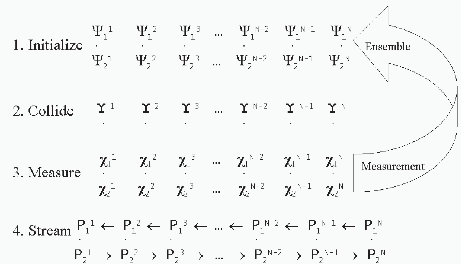
The algorithm can be summarized by four major steps, which are illustrated in figure 1. The first step encodes the initial state of the fluid by quantum mechanically setting the state of each qubit at each lattice site. The second step transforms the two-qubit product state at each lattice site to in general an entangled state, whose state is denoted by . Third one makes a projective measurement of the post-collision states , and one must repeat the first three steps to find the outgoing occupation probabilities . In the fourth and final step one streams the mass density with the appropriate post-collision occupation probabilities, from the left with particles representing positive momentum, and from the right with particles representing negative momentum, and the mass density is calculated. Subsequent time steps are identical except for a change in the initial mass density profile, i.e., initial qubit states in the first step.
III Persistent-Current Qubit
The fundamental unit of quantum logic we will use to implement the algorithm is the PC QubitPRB. It consists of a superconducting loop that is interrupted by three Josephson junctions, pictured as x’s in figure 2(a). The magnetic flux is the only control field for our qubit, and as shown in the figure, is usually denoted by where is a single flux quantum, is Planck’s constant, and is the magnitude of the charge of an electron. Physically, a Josephson junction is a small layer of insulator sandwiched between superconductors, so our system is a superconducting loop interrupted by three layers of insulator about 1nm thick. For single qubit manipulation the magnetic flux through the loop will be modified. The flux seen by a DC SQUID magnetometer, a combination of applied flux and qubit-induced flux, will serve as our measurement variable.

The Hamiltonian of the qubit is derived by considering a circuit element model of our system, which consists of three Josepshon junctions, where two junctions have the same cross-sectional area, and the third is smaller by a factor of . The constituent relations for an ideal Josephson junction are
| (3a) | ||||
| (3b) | ||||
where is the current through the junction, is the voltage across the junction, is the maximum current the junction can hold without a voltage appearing across it, =-, and is the phase of the plane wave macroscopic wavefunction that characterizes the superconductor condensate on the +,- side of the junction respectively. Note that is a function linear in the cross-sectional area of the junction, and hence the third junction has a lower by a factor of .
The energy associated with an ideal Josephson junction is found by integrating the power from time to some final time , which is equivalent to an integral from zero phase to some phase . The energy it takes to set the phase of a Josephson junction to is
| (4) |
where .
By including the charging energies due to the capacitance of the junctions, the Hamiltonian of our circuit isPRB
| (5) |
where , , , , , and . The number of degrees of freedom in the problem was reduced by the fluxoid quantization conditionTerry
| (6) |
which forces the sum of the gauge invariant phases to be proportional to the amount of flux quanta modulo an integer multiple of .
We have chosen to associate the capacitive energy, the first two terms in (5), with the kinetic energy, and the ideal Josephson energy, the last four terms in (5), with the potential energy. The potential energy is that of an infinite lattice of double wells, as seen in figure 2(b). The arrow in the plot shows the direction one would take to traverse from one side of a double well to another. The barrier between the left and right sides of a single double well is much lower than any barrier between different double wells.
Though quantum mechanics plays a foremost role in deriving the constitutive relations for the superconducting circuit elements, the Hamiltonian for the circuit itself so far has been classical. The quantum version of the circuit can be understood by imagining a phase “particle” in the potential shown in figure 2(b). The behavior of this “particle” is analogous to a particle with an anisotropic mass moving in a 2D periodic potential, and so there exist energy bands in a -space, which is here related to the charge stored capacitively by the Josephson junctions. By properly choosing , where , one can remove any (and hence charge) dependence in the energy of the system, and hence can reduce the problem to that of an effective double well. What we have done is choose parameters such that tunneling between adjacent double wells can be neglected relative to the tunneling within a double well in the tight-binding solution, making the solution effectively that of a single double well.
By considering only the lowest two levels of the double well, the equivalent Hamiltonian is
| (7) |
where are the eigenvalues of circulating current for the two eigenstates and is the tunneling element from one side of the double well to the other. The energies of the two eigenstates along with a sketch of the double well as a function of applied flux are shown in figure 3. One significant difference between this qubit and the one used in NMRQC is the presence of the term. The implication of such a term is that the energy of the eigenstates as well as the eigenstates themselves change as the bias field is modified. In figure 3 we see that at the classical degeneracy point the qubit’s eigenstates are eigenstates, while far from , but still far from , the eigenstates are those of . The same thing happens for , but now the eigenstates have switched energies, i.e., the ground state here is the first excited state of and vice versa.

The PC Qubit has some advantages over other superconducting qubits. Charge fluctuations, a consequence of trapped substrate charge, are deemed inconsequential through the choice of parameters used when designing the PC Qubit circuit. Also, flux noise has been reduced in this system over other flux qubits since this system has a smaller loop.
A typical conceptual misconception can be addressed at this point. The two different states used in computation are not related to single Cooper pair behavior. Rather, they are macroscopically distinct states described by the circulating current due to millions of Cooper pairs, characterized by different average induced fluxes when in a magnetic field.
IV Implementation with the PC Qubit
We now show how one can use the PC Qubit to simulate the 1D diffusion equation. In section IV.1 we elaborate on a scheme based upon changing the flux bias points of the qubits during the algorithm, which will lead to a very general initialization scheme, but a less general collision. In section IV.2 we discuss a more general collision, analogous to that done in NMRQC, and how to initialize the qubits before this general collision.
IV.1 The Multiple Bias Point Implementation
The first of the four steps of the algorithm is initializing each qubit at each node. As discussed in section II, each qubit must be initialized into a state of real and positive phase in its own Hilbert space. This set of states consists of all those lying on the real phase geodesic between the ground and first excited states on the Bloch sphere. The ground state of the PC Qubit as a function of applied flux coincidentally also occupies exactly this geodesic on the Bloch sphere, as discussed in section III. Initialization can thus be accomplished while staying in the ground state by adiabatically changing the applied magnetic flux, as depicted in figure 3.
The flux used to set the state of one qubit will be affected by the state of the other qubit and its bias current. This permanent inductive coupling can be accounted for by slightly adjusting the applied flux to compensate for the flux introduced by the other qubit and its bias line. All errors due to approximations made when initializing by rotating dynamically on the Bloch sphere, including errors due to decoupling, have been avoidedNMRIMP. We emphasize that the initialization portion of the algorithm is identical for any simulation, whether it be for a different equation, a multi-phase simulation, or in a different number of dimensions.
The second step of the algorithm is the collision. Here we study a very specific unitary transformation, the described in section II. This matrix simply “half-way” swaps the middle two (first and second excited) computational states of the coupled system. In NMRQC, the coupled eigenstates are exactly those computational states, but there are no direct matrix elements connecting these statesBerman. When the PC Qubits are coupled, the first and second excited states of the four-level system, denoted as and respectively, are in general not the same as the computational basis states the intends to affect. However, the dc bias fields of each qubit can be tuned to make these two sets of eigenstates coincide. Once this is done, one can then implement the by simply oscillating the magnetic field bias at the frequency corresponding to the energy difference between the middle two eigenstates. This is just a Rabi oscillation between the middle two eigenstates, and since one wants to only “half-way” swap the states, the radiation should only be left on for a quarter of a Rabi period.

Besides finding the appropriate bias points such that the middle two eigenstates of the coupled system are very similar to the middle two computational states, one must also verify that the coupling between these states in the presence of an oscillating magnetic field is non-zero. The results of these calculations are shown in figure 4. The bias point of qubit 1, , must be chosen to be far from 1/2, but not too far. In these calculations we take . In the figure we see that when qubit 2 is biased at around , the first two system excited states are very similar to the middle two computational states, with overlap elements of about 0.97. At this same bias point one sees a Rabi matrix element of about 0.02, which is more than sufficient for our purposes.
This approximate swap has been incorporated into simulation of the FQLGA for the 1D diffusion equation and the results are pictured in figure 5. Snapshots of three different times have been shown, for both an ideal simulation and one including the error introduced due to the approximate collision. At time one can see that we have initialized our fluid to a gaussian profile. Later time steps of the ideal implementation show the expected spreading due to diffusion, while conserving the total number of particles. Increase in the diffusion constant of the approximate collision when compared to the ideal simulation results from the enhanced population in the , , and states relative to the state due to extra matrix elements in the approximate swap that couple the four states.

Even with an ideal swap operator, an interesting timing issue arises upon non-adiabatically switching the bias fields from the initialization settings to the proper settings to do a Rabi oscillation between the two middle product states. We first illustrate this timing issue and then show how it can be made negligible by making a larger ensemble measurement.
Once the applied fluxes are changed to those appropriate to perform the approximate swap, the initialized states will most likely not be eigenstates anymore, and hence will begin to precess due to a time-independent perturbation. Assuming things can not be accurately controlled at these timescales, one will have now introduced a random phase difference between the two qubits due to this Larmor precession. This effect is pictured in figure 6. The states before the bias fields are switched lie along the same geodesic. Upon changing the magnetic flux seen by each qubit, the qubits begin to precess, out of phase.
The effect of this phase difference on the algorithm will be to alter the fraction of particles at each lattice site, post-collision, that are “moving” to the right and to the left. The results of measuring the post-collision occupation probabilities having accounted for a constant phase difference is summarized by
| (8a) | |||
| (8b) | |||
The effect of this error on the simulation is effectively averaged away when an ensemble is measured, since is randomly different for each member of the ensemble. These results are shown in figure 7. One can see small random deviations from the ideal simulation that can be made infinitesimally small by measuring a larger ensemble (an ensemble average of 1000 repeated measurements was simulated here).


In summary, an initialization scheme has been developed that is not available to qubits with only one term in their Hamiltonian. This initialization scheme is limited only by the precision of the current source used to create the magnetic field that biases the qubit. The scalability of this scheme relative to those used in NMRQC is an interesting question, but is not resolved here. The collision implementation is also unique to qubits with multiple term Hamiltonians, but the unitary transform implemented is unique to the diffusion equation, and fortuitously simple. A collision scheme that could be generalized to any unitary transformation would be much more useful.
IV.2 Generalized NMRQC-like Implementation
Generalization of the above implementation to any fluid dynamics, i.e., any unitary transformation, can be done in an analogous way to NMRQC schemes. Generalization of the collision transformation consists of using a universal set of quantum computation gates, and decomposing all transformations into a sequence of theseChuang. In NMRQC collision is performed by a sequence of single qubit unitary transformations and coupled free evolution. In this section we will begin by discussing the single qubit rotations needed for a general decomposition, and briefly mention the role they could play in initialization. We will then explore the free evolution of a coupled PC Qubit system, and then show how to combine the single and coupled pulses to implement the collision of the 1D FQLGA for the diffusion equation.
Single qubit transformations can most easily be achieved in a rotating frame, since here the frequency of precession can be much lower than the Larmor time scale. For this implementation we will only study the case where our qubit is biased at . This discussion is easily generalized to any bias point, but the mathematical notation can get quite cumbersome. The Hamiltonian of the PC Qubit in an applied AC field is
| (9) |
where is the frequency of the applied field, is proportional to the amplitude of the applied field, is the phase of the applied field, and .
In the frame rotating about this Hamiltonian becomes
| (10) |
The quantum state will now precess in this frame about the axis defined by , with the angle through which the state has precessed given by . It will be convenient to only consider the set of two rotations defined by and , which are rotations about and respectively. These rotations, denoted as () and () respectively, can be used in conjunction to bring the qubit state to any point on the Bloch sphere in the rotating frame.
One can use these single qubit rotations not only as part of the collision, but also for initializing, since they can bring the qubit state to anywhere on the Bloch sphere. As already discussed in section IV.1, the ground state of a coupled PC Qubit system is not in general the product of single qubit ground states. Thus, when initializing a qubit via () and (), one is not starting rotation from the single qubit ground state. However, since the ground state is very close to a product of single qubit ground states, this difference is nearly negligible. In figure 8 we show the effects of incorporating this error into the algorithm when the coupling constant is taken to be 1/10 of the qubit resonant frequencies, a rather exaggerated estimate since the coupling is usually much smaller. The diffusion constant is decreased by this approximation, due to the enhanced population in the state relative to the state from the coupling.

The other gate operation needed to form a universal set for general decomposition is coupled free evolution. The first thing to do is go to a co-rotating frame where one can have a coupled Hamiltonian only, i.e., no single qubit terms, that is time-independent. In NMRQC this is done by going to the frame where both qubits are rotated around the axis. However, since our coupling does not commute with our single qubit terms, a different method will be used. For notational convenience only, we consider the case where both qubits are biased at , where our Hamiltonian is
| (11) |
In the co-rotating frame where both qubits are rotating around the axis, one has the Hamiltonian
| (12) |
as long as . This constraint of imposes limitations on some NMRQC initialization schemes which use frequency selective initialization.
One can now rewrite the unitary collision transformation in the following suggestive way:
| (13) |
The first term is just free evolution in the co-rotating frame. The second term can be written as:
| (14) |
where the middle term can be written as:
| (15) |
Hence one can perform a decomposition of the collision transformation into a sequence of single qubit rotations and coupled free evolution.
In summary, we have shown that the PC Qubit can implement the unitary transform that performs collisions in the 1D FQLGA for the diffusion equation by a single and coupled qubit evolution decomposition. The single qubit rotations were shown to be feasible for qubit initialization as well, with a slight approximation due to the coupled ground state that is not a product state. The coupled free evolution was seen to require identical qubit frequencies over a lattice site, making initialization a bit more challenging.
V Conclusions
In this paper we have shown that the implementation of the FQLGA for the 1D diffusion equation is feasible with PC Qubits. We began by considering the simplest scheme possible using the PC Qubit. This consisted of first initializing the qubits while keeping them in their ground state, and then performing the collision by quickly changing their flux bias points and then performing a single pulse. This initialization technique could prove useful, but the way we have implemented the collision is not easily generalized to other collisions. We needed to develop a more general collision scheme, and then see how we could initialize in conjunction with that new scheme.
A more general collision transformation was then discussed by decomposing the unitary matrix into a sequence of single qubit rotations and coupled free evolution. We first developed single qubit rotations for the PC Qubit that could be used as part of the collision decomposition as well as for initializing the occupation probabilities. The initialization was considered only approximate due to the permanent non-commuting coupling between qubits. For the coupled free evolution we saw that transforming to a rotating frame analogously to NMRQC set a strong but feasible constraint on the frequencies of our qubits. Ultimately one would like to remove the constraint of equal frequencies, so that frequency-selective initialization can be done analogously to the NMRQC implementation, alongside the very general collision scheme. One would then also need to account for initialization pulses rotating states from a non-product ground state.
Acknowledgements.
The authors would like to thank Debra Chen and Jeff Yepez for valuable discussions. This work is supported by the AFOSR/NM grant FA 9550-04-1-0221.References
- (1) K. Berggren, Quantum Computing with Superconductors, Proc. IEEE Vol. 92, No. 10, 1630(2004).
- (2) M. A. Nielsen and I. L. Chuang, Quantum Computation and Quantum Information, Cambridge Univ. Press(2000).
- (3) J. Yepez, in Quantum Computing and Quantum Communications Lecture Notes in Computer Science, Vol. 1509, Springer-Verlag 35(1999).
- (4) D. A. Wolf-Gladrow, Lattice-Gas Cellular Automata and Lattice Boltzmann Models, Edited by A. Dold et al., Springer(2000).
- (5) J. Yepez, An efficient quantum algorithm for the one-dimensional Burgers equation, quant-ph/0210092.
- (6) I. Chiorescu, et al., Coherent Dynamics of a Superconducting Flux Qubit, Science 299, 1869(2003).
- (7) J. R. Friedman et al., Quantum Superposition of Distinct Macroscopic States, Nature 406, 43(2000).
- (8) Y. A. Pashkin et al., Quantum Oscillations in Two Coupled Charge Qubits, Nature 421, 823(2003).
- (9) J. M. Martinis et al., Rabi Oscillations in a Large Josephon-Junction Qubit, Phys. Rev. Lett. 89, 117901(2002).
- (10) D. Vion et al., Manipulating the Quantum State of an Electrical Circuit, Science 296, 886(2002).
- (11) I. L. Chuang et al., Bulk Quantum Computation with Nuclear Magnetic Resonance: Theory and Experiment, Proc. R. Soc. Lond. A 454, 447(1998).
- (12) M. Pravia et al., Experimental Demonstration of Quantum Lattice Gas Computation, Quantum Information Processing Vol. 2(2003).
- (13) J. Yepez, Quantum Lattice-Gas Model for the Diffusion Equation, Intl. Jour. of Mod. Phys. C Vol. 12, No. 9, 1285 (2001).
- (14) T.P. Orlando et al., Superconducting Persistent-Current Qubit, Phys. Rev. B 60, 15398(1999).
- (15) T.P. Orlando, K.A. Delin, Foundations of Applied Superconductivity, Addison-Wesley(1991).
- (16) G. P. Berman et al., Simulation of the Diffusion Equation on a Type-II Quantum Computer, Physical Review A 66, 012310(2002).