Entanglement and non-locality are different resources

Let’s focus more specifically on the first case of interest for this paper, $m_{A}=m_{B}=3$. The no-signaling probability space is 15-dimensional. All the facets of the deterministic polytope are known [20]: up to relabelling of the settings and/or of the outcomes, they are equivalent either to the usual two-settings CHSH inequality, or to the truly three-settings inequality $I_{3322}$ that reads

Here the notation represents the coefficients that are put in front of the probabilities, according to

The maximal violation allowed by QM is obtained for the singlet and is $\langle I_{3322}\rangle=\frac{1}{4}$. To become familiar with the notations, the deterministic strategy in which Alice outcomes $r_{A}=0$ for $A_{0},A_{1}$ and $r_{A}=1$ for $A_{2}$, and Bob outcomes always $r_{B}=0$, corresponds to the probability point

To see the result of $I_{3322}$ on this strategy, one has simply to multiply the arrays term-by-term: here we find $I_{3322}=0$. There are obviously $2^{6}=64$ deterministic strategies; among these, 20 saturate the inequality $I_{3322}=0$ (i.e., they lie on the facet) while the others give $I_{3322}<0$. To verify that this is indeed a facet, it is enough to show that the rank of the matrix containing the 20 points that saturate the inequality is $d_{ns}-1=14$, so that the condition $I_{3322}=0$ really defines a hyperplane [21].

The NLM is defined as a two-input and two-output channel. Alice inputs $x$ and gets the outcome $a$, Bob inputs $y$ and gets the outcome $b$; all these numbers take the values 0 or 1, the marginal distribution on each side is completely random, $P(a=0)=P(b=0)=\frac{1}{2}$, but the outcomes are correlated as

Explicitly, if either $x=0$ or $y=0$, then $(a,b)=(0,0)$ or $(1,1)$ with equal probability; if $x=y=1$, then $(a,b)=(0,1)$ or $(1,0)$ with equal probability.

The most general strategy allowing a single use of the NLM is sketched in Fig. 2. Alice and Bob share some random variable $\lambda$. Alice inputs in the machine the bit $x=x(A_{i},\lambda)$; the machine gives the output $a$, and Alice outputs $r_{A}=r_{A}(A_{i},\lambda,a)$. The extremal strategies are such that a given $x$ is associated to each $A_{i}$, and the outcome is either $r_{A}=a$ or $r_{A}=1-a$. Similarly for Bob. Note that it is also possible that for a given pair $(A_{i},B_{j})$ Alice uses the machine while Bob outputs a deterministic bit; in this case, we can suppose that Bob inputs $y=0$ in the machine but does not use the output $b$. We shall come back below to the listing of extremal strategies. Let’s now see how the polytope of possible probability distributions is enlarged by allowing a single use of the NLM.

By construction, with a single use of the machine one can violate the CHSH inequality more than is possible in QM. In the polytope picture, one new point appears above any face corresponding to CHSH: the facets of the enlarged polytope should now pass through this points. They must pass through the deterministic points as well, because these points are still extremal. All this is sketched in Fig. 1. We won’t study this example longer, however, since there is no hope of finding something interesting above a CHSH-like facet: all the probability distributions involving two settings which are no-signaling (in particular all distributions arising from measurements on a quantum state) can be simulated by a single use of the NLM [18].

So let’s consider the facet defined by $I_{3322}=0$. Again, a single use of the NLM allows to violate $I_{3322}$, which is expected since the NLM can in particular simulate the singlet. For instance, consider the strategy in which Alice inputs $x=0$ in the NLM for $A_{0}$ and $A_{1}$, and $x=1$ for $A_{2}$, while Bob inputs $y=0$ for $A_{0}$ and $B_{2}$, and $y=1$ for $B_{1}$; in each case, the outputs are $r_{A}=a$, $r_{B}=b$. This strategy gives the probability point

yielding $I_{3322}=\frac{1}{2}$: the machine can violate $I_{3322}$ more than QM. However here, we are going to show what is graphically represented in Fig. 1: for non-maximally entangled states, some points achievable with quantum states lie outside the enlarged polytope. In other words, the facets of this polytope define generalized Bell’s inequalities that can still be violated by QM.

To find the facets of the polytope allowing a single use of the machine, one must first list all the vertices (extremal strategies). This can be done systematically on a computer, once having noticed that for each setting, Alice and Bob have six choices: deterministically output 0 or 1 (noted $0_{d}$, $1_{d}$), input $0$ or $1$ in the machine and keep the output of the machine (noted $0_{m}$, $1_{m}$), input $0$ or $1$ in the machine and flip the output of the machine (noted $0_{f}$, $1_{f}$) [22]. This listing gives a priori $6^{6}=46656$ strategies, although many of them are equal [23] and only 3088 different strategies are left after inspection. Note that some of these are not even extremal points of the polytope: for instance, the strategy $[0_{m},0_{m},0_{m};0_{m},0_{m},0_{m}]$, in which both Alice and Bob input 0 in the NLM for all settings, yields the same probability point as the equiprobable mixture of the deterministic strategies $[0_{d},0_{d},0_{d};0_{d},0_{d},0_{d}]$ and $[1_{d},1_{d},1_{d};1_{d},1_{d},1_{d}]$. Certainly not equivalent to a mixture of deterministic strategies, however, are those strategies like (III.2) which violate $I_{3322}$: upon counting, there are 28 of these, all giving the same violation $I_{3322}=\frac{1}{2}$. To find the facets of the new polytope, we use available computer programs [24]. We find some trivial facets, plus a single non-trivial one [25] which reads

This new inequality is extremely similar to $I_{3322}$, eq. (III.1): only the coefficient of $P_{0}(r_{A}=0)$ is now $-2$ instead of $-1$. The origin of this difference can be appreciated, at least to some extent: one of the biggest difficulties found in adapting the Toner-Bacon model [4] to non-maximally entangled states lies in the need of simulating not only the correlations, but also the non-trivial marginal distributions. It is thus a good idea for our purpose, to add penalties on the marginal distributions.

Summarizing, we have found a tight inequality $M_{3322}\leq 0$ which is satisfied by all the 3088 extremal points of the polytope of probabilities achievable by shared randomness plus a single use of the NLM. Now we move on to show that QM violates this inequality.

We consider states of the form

with $\cos\alpha\geq\sin\alpha\geq 0$. Up to local operations, this is the most general pure state of two qubits (Schmidt decomposition). We form the Bell operator ${\cal M}$ as usual, by replacing the probabilities in (III.2) by the corresponding one-dimensional projectors, like

For each $\alpha$, we have to find the settings which maximize $M(\alpha)=\mbox{$\langle\psi(\alpha)|{\cal M}|\psi(\alpha)\rangle$}$. We have not found a closed analytical formula, but it is easy for a computer to optimize over twelve real parameters. The result is shown in Fig. 3: one finds $M(\alpha)>0$ for $0<\alpha\lesssim\frac{2}{19}\pi$, with a maximal violation $M(\bar{\alpha})\approx 0.0061$ at $\bar{\alpha}\approx 0.0712\,\pi$. It appears that all the optimal settings are of the form $\hat{a}_{i}=\cos\theta_{A}^{i}\hat{z}+\sin\theta_{A}^{i}\hat{x}$, $\hat{b}_{j}=\cos\theta_{B}^{j}\hat{z}+\sin\theta_{B}^{j}\hat{x}$.

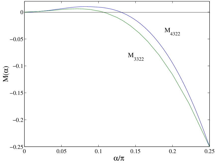
The curve of Fig. 3 is the exact version of the pictorial argument of Fig. 1. Note in particular the following features: (i) As expected, there is no violation for the singlet ($\alpha=\frac{\pi}{4}$), because this state can be simulated with the NLM; even more, $M(\frac{\pi}{4})=-\frac{1}{4}$ which is the difference between $\langle I_{3322}\rangle=\frac{1}{4}$ on the singlet and the maximal value $I_{3322}=\frac{1}{2}$ achievable with the NLM. The picture of Fig. 1 yields in this case even a quantitative prediction. (ii) As mentioned [19], it is not obvious that the set of probabilities obtained from quantum measurements on $|\psi(\alpha)\rangle$ is convex; so at this point it is not proved that states arbitrarily close to the product state $|00\rangle$ can’t be simulated by a single use of the NLM — the proof will be provided in Section IV.

As we mentioned in the introduction, two bits of communications are a sufficient resource to simulate any state of two qubits. The analog simulation using twice the NLM is still missing, and may even not exist. While waiting for more clarification, we have found a way of violating inequality (III.2) by using the NLM twice. The settings are coded as $A\to(x^{\prime},x^{\prime\prime})$, $B\to(y^{\prime},y^{\prime\prime})$ according to: $A_{0}\to(0,0)$, $A_{1}\to(0,1)$, $A_{2}\to(1,0)$; $B_{0}\to(0,0)$, $B_{1}\to(1,0)$ and $B_{2}\to(0,1)$. Then, $x^{\prime}$ and $y^{\prime}$ are used as inputs in the first use of the machine, whose outcomes are denoted $a^{\prime}$ and $b^{\prime}$; $x^{\prime\prime}$ and $y^{\prime\prime}$ are used as inputs in the second use of the machine, whose outcomes are denoted $a^{\prime\prime}$ and $b^{\prime\prime}$. Finally, Alice outputs $r_{A}=a^{\prime}+a^{\prime\prime}$, Bob outputs $r_{B}=b^{\prime}+b^{\prime\prime}$ (sum modulo 2). This strategy gives the probability point

yielding $I_{3322}=1$ and $M_{3322}=\frac{1}{2}$.

We can go a step further. Consider a mixture of two strategies: with probability $p$, the strategy just described which uses two NLMs; with probability $1-p$, the deterministic strategy in which Alice and Bob output always $r_{A}=r_{B}=1$ for all settings (all entries of the table are zeros), and which obviously does not require any use of the NLM. Such a mixed strategy yields a violation $M_{3322}=\frac{p}{2}$ of the inequality. Now, if $p<\frac{1}{2}$, this strategy uses less than one NLM on average [27]. This is not a contradiction with our main result: at least two NLMs must be available to simulate non-maximally entangled states, albeit possibly this resource is not used for all items.

It is natural to ask whether inequality (III.2) provides also a Bell inequality for one bit of communication. Bacon and Toner [26] had studied such inequalities for three settings, but they restricted to correlation inequalities, whereas inequality (III.2) is a probability inequality. The problem is complex because, as we mentioned, pure strategies with one bit of communication imply signaling; we must find a mixture of such strategies which is no-signaling and which violates our inequality. It turns out that such mixtures do exist, so that our inequality is not an inequality for one bit of communication. In other words, the polytope of the probability distributions obtained with one bit of communication plus the no-signaling constraint is larger than the one associated to a single use of the NLM.

As an explicit example [27], it can be verified that the no-signaling strategy

yields the violation $M_{3322}=\frac{1}{5}$ and can be obtained as the equiprobable mixture of the following five one-bit strategies:

In these notations, $c_{i}$ is the value of the bit that Alice sends to Bob when she has used the setting $A_{i}$; $r_{B_{j}}=c$ means that, upon choosing the setting $B_{j}$, Bob outputs the value of the bit received from Alice.

The fact that the inequality (III.2) can be violated by one bit of communication shows that a single use of the NLM does not correspond to a single bit of communication plus no-signaling: the NLM is a resource strictly weaker than communication, as argued in Ref. [10], and grasps finer details of the structure of quantum non-locality. The question whether one bit of communication is sufficient to simulate non-maximally entangled states is obviously still open.

In the case $m_{A}=4$ and $m_{B}=3$, the no-signaling probability space is 19-dimensional. All the facets of the deterministic polytope have been listed in Appendix A of Ref. [20]: one finds of course CHSH, $I_{3322}$, plus three new inequalities. The one which turns out to be of interest is (A2) of that reference [28]; using the properties of no-signaling distributions, and providing Alice instead of Bob with the four settings, this inequality can be re-written in the form

The polytope of a single use of the NLM can be found as in Section III. After listing, one finds that the $6^{7}$ possible extremal strategies produce 17272 different points, 63 of which violate (IV.1) by $I^{(2)}_{4322}=\frac{1}{2}$. By numerical inspection [29], we found that these points define a single non-trivial new facet

Quite similarly to the case $m_{A}=m_{B}=3$, the difference between the original inequality and the new one is just a larger penalty on one marginal. Also similar is the fact that (IV.1) can be violated by strategies which use twice the NLM or one bit of communication, as can be easily verified. In fact, simply by taking the corresponding strategies of Section III and adding the condition $A_{3}=A_{1}$, we can produce the probability point

which gives $M_{4322}=\lambda$, with $\lambda=\frac{1}{2}$ in the case of two NLMs and $\lambda=\frac{1}{5}$ in the case of one bit of communication.

The interest of $M_{4322}$ comes from the quantum violation, which (i) is larger than the violation of $M_{3322}$, thus allowing to extend the range of $\alpha$ for which one NLM is not enough, and (ii) is obtained for a family of settings which can be easily parametrized (see Appendix A). Specifically, one finds $M(\alpha)>0$ for $0<\alpha\lesssim\frac{\pi}{7.8}$, with a maximal violation $M(\bar{\alpha})\approx 0.0102$ at $\bar{\alpha}\approx\frac{\pi}{12}$ (Fig. 3). For small values of $\alpha$, moreover, one can prove

Thus $M(\alpha)>0$ as soon as $\alpha>0$: the simulation of pure states with arbitrarily weak entanglement requires more than one NLM — again, as we noticed at the end of paragraph III.4, it may be the case that correlations can be reproduced by using this resource only on a subset of the particles.

Beyond the $3322$ and $4322$ cases, the facets of the deterministic polytope have not been listed exhaustively, but several examples of facets are available [20, 30]. On these, we searched for possible extensions of our results by increasing the penalties in some marginals.

Starting from the inequality $I_{4422}\leq 0$ given in Ref. [20], the corresponding inequality $M_{4422}\leq 0$ is obtained exactly as above, just replacing $-1$ with $-2$ as the coefficient of $P_{0}(r_{A}=0)$.The result is similar: $M_{4422}\leq 0$ indeed holds for all strategies allowing a single use of the NML, and QM violates it. If all the four settings are used, the range of values of $\alpha$ in which we found a violation is however smaller than for $M_{3322}$, only up to $\sim\frac{\pi}{13}$. Note that $I_{4422}$ is less violated than $I_{3322}$ by the singlet [20], while the violation achievable by the NLM is $\frac{1}{2}$ for both; by looking at Fig. 1, it becomes intuitive that the range of violation should decrease. Interestingly, one can recover the (better) result of Fig. 3 by setting $a_{3}$ and $b_{0}$ to the value $1_{d}$, thus reducing $M_{4422}$ to $M_{3322}$. This assignment reads $P_{3}(r_{A}=0),P_{0}(r_{B}=0)\rightarrow 0$ and is thus not of the form (27): it describes a degenerate measurement.

Other 4422 deterministic facets, as well as some 5522 and 6622 ones, did not appear to be worth a closer study after our survey. We have considered neither inequalities with larger number of outcomes, nor multi-partite scenarios.

References

- [1] A. Einstein, B. Podolski, N. Rosen, Phys. Rev. 47, 777 (1935); J.S. Bell, Physics 1, 195 (1964)
- [2] A. Tapp, R. Cleve, G. Brassard, Phys. Rev. Lett. 83, 1874 (1999)
- [3] B. Gisin, N. Gisin, Phys. Lett. A 260, 323 (1999); M. Steiner, Phys. Lett. A 270, 239 (2000)
- [4] B. F. Toner, D. Bacon, Phys. Rev. Lett. 91, 187904 (2003)
- [5] S. Popescu, D. Rohrlich, Found. Phys. 24, 379 (1994)
- [6] B.S. Tsirelson, Hadronic J. Supplement 8, 329 (1993)
- [7] J.F. Clauser, M.A. Horne, A. Shimony, R.A. Holt, Phys. Rev. Lett. 23, 880 (1969)
- [8] W.van Dam, quant-ph/0501159
- [9] S. Wolf, J. Wullschleger, quant-ph/0502030
- [10] N. J. Cerf, N. Gisin, S. Massar, S. Popescu, quant-ph/0410027
- [11] V. Scarani, W. Tittel, H. Zbinden, N. Gisin, Phys. Lett. A 276, 1 (2000); V. Scarani, N. Gisin, quant-ph/0410025
- [12] H. Zbinden, J. Brendel, N. Gisin, W. Tittel, Phys. Rev. A 63, 022111 (2001); A. Stefanov, H. Zbinden, N. Gisin, A. Suarez, Phys. Rev. Lett. 88, 120404 (2002)
- [13] P. Eberhard, Phys. Rev. A 47, R747 (1993)
- [14] A. Acín, T. Durt, N. Gisin, J.I. Latorre, Phys. Rev. A 65, 052325 (2002)
- [15] S. Pironio, Phys. Rev. A 68, 062102 (2003)
- [16] J. Barrett, Phys. Rev. A 65, 042302 (2002)
- [17] I. Pitowski, Quantum Probability, Quantum Logic, Lecture Notes in Physics 321 (Springer Verlag, Heidelberg, 1989)
- [18] J. Barrett, N. Linden, S. Massar, S. Pironio, S. Popescu, D. Roberts, Phys. Rev. A 71, 022101 (2005)
- [19] This statement is valid for the set of all possible measurements on all possible quantum states, see Ref. [17], as well as paragraph V.C of: R.F. Werner, M.M. Wolf, Phys. Rev. A 64, 032112 (2001); and references therein. If one restricts to the measurements on a given state, or even to the von-Neumann measurements on a Hilbert space with given dimension, convexity is not proved (although no counter-example is known, to our knowledge).
- [20] D. Collins, N. Gisin, J. Phys. A: Math. Gen. 37 1775 (2004)
- [21] L. Masanes, Quant. Inf. Comput. 3, 345 (2003)
- [22] This takes automatically into account the possibility that Alice and Bob use the alternative version of the NLM defined by .
- [23] For instance, and define the same probability point.
- [24]
We used the function
convhullnof Matlab on the 28 points which yield alone, or on these points plus some of the 20 deterministic points which yield . The result is the same. - [25] Actually, the program outputs two facets: inequality (III.2), and a similar one where the first line (2,0,0) is replaced by (1,1,0). If one writes down the inequality explicitly, it becomes evident that one is transformed into the other by exchanging and and by flipping the bit .
- [26] D. Bacon, B.F. Toner, Phys. Rev. Lett. 90, 157904 (2003)
- [27] This point was pointed out to us by S. Pironio (private communication).
- [28] Actually, we did not perform a systematic search because the polytope becomes rather big. Based on the result of Section III, we have taken inequalities (A1)-(A3) of [20], verified that all of them can be violated by a single use of the NLM, then modified the marginals. It turns out that, even by modifying the marginals by 1, the new inequalities derived from (A1) and (A3) are not violated by QM.
- [29]
Finding a polytope given 63 vertices is too hard a task
for the function
convhullnof Matlab. Therefore, we have run this function more than one million of times, each time randomly selecting 30 points out of the 63. When the selected points defined a non-trivial facet, it was invariably (IV.1). Thus we are confident that this is the only interesting inequality for one use of the NLM above the deterministic facet. - [30] D. Collins, private communication.