跳到论文正文
W Papers独立论文阅读器 arXiv:quant-ph/0412053 论文正文 计算阅读时间 · 0%
引用这篇论文根据当前论文元数据生成,正式投稿前建议核对。


License: Assumed arXiv.org perpetual non-exclusive license
arXiv:quant-ph/0412053v2 [quant-ph] 16 Nov 2005

Quantum state estimation and large deviations

M. Keyl Thanks: Electronic Mail: m.keyl@tu-bs.de Affiliation: [1ex] Istituto Nazionale di Fisica della Materia, Unita’ di Pavia, Affiliation: Dipartimento di Fisica “A. Volta”, via Bassi 6, I-27100 Pavia, Italy
August 11, 2026
Abstract

In this paper we propose a method to estimate the density matrix ρ\rho of a dd-level quantum system by measurements on the NN-fold system in the joint state ρ⊗N\rho^{\otimes N}. The scheme is based on covariant observables and representation theory of unitary groups and it extends previous results concerning pure states and the estimation of the spectrum of ρ\rho. We show that it is consistent (i.e. the original input state ρ\rho is recovered with certainty if N→∞N\to\infty), analyze its large deviation behavior, and calculate explicitly the corresponding rate function which describes the exponential decrease of error probabilities in the limit N→∞N\to\infty. Finally we discuss the question whether the proposed scheme provides the fastest possible decay of error probabilities.

1 Introduction

The density operator ρ\rho of a dd-level quantum system (d∈ℕd\in\mathbb{N}) describes the preparation of the system in all details relevant to statistical experiments, and the task of quantum state estimation is to determine ρ\rho by measurements on a (possibly large) number NN of systems, which are all prepared according to ρ\rho. In the limit of infinitely many input systems it is of course possible to get exact estimates. If NN remains finite, however, estimation errors are unavoidable. The best we can get (if NN is large enough) is an estimation scheme which produces only small errors or, better to say, which produces large errors only with a small probability.

There are several ways to get “good” estimation schemes. One possibility is to choose an appropriate figure of merit which measures the quality of the estimates (e.g. averaged fidelities with respect to the original density matrix) and to solve the corresponding optimization problem. If we know a priori that the input state ρ\rho is pure (but otherwise unknown) this approach is very successful and leads to optimal estimators, which can be given in closed form for all finite values of NN; cf. e.g. [24, 30, 6, 11, 19, 29, 7]. In the general case, however (i.e. if nothing is known about ρ\rho) the situation is much more difficult. First of all the result depends much more on the figure of merit chosen than in the pure state case, and even if we have found an appropriate quality criterion it is in general very hard to determine the corresponding optimal estimator explicitly for arbitrary NN; some results related to this approach can be found in [36, 15, 2].

A way out of this dilemma, is to neglect the quality of the estimates for finite NN and to look for estimation schemes which guarantee at least that error probabilities vanish “as fast as possible” as NN goes to infinity (cf. [22, 24]; for a collection of recent publications on the subject see also [18]). There are two approaches which implement this somewhat vague idea in a mathematically exact way. One possibility is to look at variances (rescaled by NN) in the limit N→∞N\to\infty. This is done in several works (cf. e.g. [17, 16, 31] and in particular the papers reprinted in [18]) and it leads to quantum analogs of classical Cramer-Rao type bounds. The second idea is to analyze the large deviation behavior of the estimators. To make this more precise let us denote an estimate derived from a measurement on NN systems in the joint state ρ⊗N\rho^{\otimes N} by σ\sigma. Then we can look at the probability PN,ϵP_{N,\epsilon} that the trace-norm distance between ρ\rho and σ\sigma (or any other appropriate distance measure for states) is at least ϵ\epsilon, i.e. ‖ρ−σ‖1≥ϵ\|\rho-\sigma\|_{1}\geq\epsilon. Since ρ=σ\rho=\sigma would be the exact estimate this is clearly an error probability. Now we are interested in those cases where PN,ϵP_{N,\epsilon} vanishes exponentially fast in NN, i.e.

PN,ϵ≈CNexp(−Ninf‖ρ−σ‖1≥ϵI(σ,ρ)).P_{N,\epsilon}\approx C_{N}\exp\bigl(-N\inf_{\|\rho-\sigma\|_{1}\geq\epsilon}\,I(\sigma,\rho)\bigr). (1)

Here CNC_{N}, N∈ℕN\in\mathbb{N} is an unknown sequence of positive real numbers, growing at most subexponentially with NN (and which is of no interest for the following), and I⁡(ρ,σ)I(\rho,\sigma) is a positive function which vanishes iff σ=ρ\sigma=\rho holds. II is called the rate function because it describes the exponential rate with which estimation errors vanishes asymptotically. In classical statistics this analysis was initiated by Bahadur [3, 4, 5] and has become in the mean time a classical topic (“Bahadur efficiency”). About the quantum case, however, much less is known, and the results available so far cover three different areas: 1. In [27, 1, 21] an explicit scheme to estimate the spectrum of ρ\rho is proposed and its rate function is calculated. The latter is shown to be optimal in [20]. 2. The rate function of the optimal pure state estimator is calculated in [19]. 3. In [20] the behavior of quantities like limϵ→0inf‖ρ−σ‖1≥ϵI⁡(ρ,σ)\lim_{\epsilon\to 0}\inf_{\|\rho-\sigma\|_{1}\geq\epsilon}I(\rho,\sigma) is analyzed for one-parameter families of states, and the relation to quantum Fisher information is discussed.

The purpose of the present paper is to extend the results about the spectrum in [27] and about pure states in [19] in two respects. Firstly, we will propose a scheme to estimate the full density matrix which is based on covariant observables [24] and which reduces to [27] if we look only at the spectrum of ρ\rho. And secondly, we will pose the question whether the proposed scheme is “asymptotically optimal”, i.e. whether its rate function is bigger than the rate function of any other scheme. There is of course no guarantee that a given set of functions admits a maximal element, but in the classical case it is known that such an “optimal rate function” exists (and is given by the classical relative entropy – this is again a consequence of Bahadur’s work [3, 4, 5]). For quantum systems, however, the situation is – not very surprisingly – much more difficult.

The outline of the paper is as follows: In Section 2 we will give a more formal introduction to the questions we are considering and in 3 we will state our main results. The proofs and a more detailed discussion is then distributed among Section 4 (were we will consider U⁡(d)\operatorname{U}(d)-covariant estimation schemes) and Section 5 (where upper bounds on rate functions will be discussed).

2 Basic definitions

In this section we will present some mathematical preliminaries (in particular basic definitions and terminology) concerning quantum state estimation. A short summary of material from the theory of large deviations used throughout this paper can be found in Appendix A.

2.1 State estimation

Let us consider the dd-dimensional Hilbert space ℋ=ℂd\mathcal{H}=\mathbb{C}^{d} and the corresponding set 𝒮\mathcal{S} of density operators. The task of quantum state estimation is to determine a state ρ∈𝒮\rho\in\mathcal{S} by a measurement on an NN-fold system, which is prepared in the joint state ρ⊗N\rho^{\otimes N}. Mathematically this can be described by a normalized POV measure ENE_{N} on the state space 𝒮\mathcal{S} with values in the algebra ℬ⁡(ℋ⊗N)\mathcal{B}(\mathcal{H}^{\otimes N}) of (bounded) operators on ℋ⊗N\mathcal{H}^{\otimes N}. More precisely, ENE_{N} is a (strongly) σ\sigma-additive set function

EN:𝔅⁡(𝒮)→ℬ⁡(ℋ⊗N)​with​EN​(Δ)≥0,EN​(∅)=0,EN​(𝒮)=1​I,E_{N}:\mathfrak{B}(\mathcal{S})\to\mathcal{B}(\mathcal{H}^{\otimes N})\ \text{with}\ E_{N}(\Delta)\geq 0,\ E_{N}(\emptyset)=0,\ E_{N}(\mathcal{S})={{\rm 1\mkern-4.8muI}}, (2)

on the Borel σ\sigma algebra 𝔅⁡(𝒮)\mathfrak{B}(\mathcal{S}) of 𝒮\mathcal{S}, and the probability to get an estimate in a Borel set Δ⊂𝒮\Delta\subset\mathcal{S} is given by

μN,ρ​(Δ)=tr⁡(ρ⊗N​EN​(Δ)).\mu_{N,\rho}(\Delta)=\operatorname{tr}\bigl(\rho^{\otimes N}E_{N}(\Delta)\bigr). (3)

Since the number NN of systems is arbitrary, we need a whole sequence of observables and we will call each such sequence in the following a full estimation scheme. For a good estimation scheme the quality of the estimates should increase with NN, i.e. the error probability should decrease and in the limit of infinitely many input systems the estimate should be exact; in other words the sequence of probability measures (μN,ρ)N∈ℕ(\mu_{N,\rho})_{N\in\mathbb{N}} should converge for each ρ\rho weakly to the point measure concentrated at ρ\rho. Such an estimation scheme is called consistent.

If we are interested not in the whole state but only in some special properties of ρ\rho (e.g. its von Neumann entropy), described by a function 𝒮∋ρ↦p⁡(ρ)∈X\mathcal{S}\ni\rho\mapsto p(\rho)\in X taking its values in a locally compact, separable metric space XX we have to consider more generally POV measures EN:𝔅⁡(X)→ℬ⁡(ℋ⊗N)E_{N}:\mathfrak{B}(X)\to\mathcal{B}(\mathcal{H}^{\otimes N}) on XX instead of 𝒮\mathcal{S}. As before, tr⁡(ρ⊗N​EN​(Δ))\operatorname{tr}\bigl(\rho^{\otimes N}E_{N}(\Delta)\bigr) is the probability to get an estimate in Δ⊂X\Delta\subset X. Estimating the spectrum of a density operator is a particular example of this kind. In this case pp coincides with

s:𝒮→Σ={x∈[0,1]d|x1≥⋯≥xd≥0,∑j=1dxj=1}s:\mathcal{S}\to\Sigma=\{x\in[0,1]^{d}\,|\,x_{1}\geq\cdots\geq x_{d}\geq 0,\sum_{j=1}^{d}x_{j}=1\} (4)

which maps a density operator ρ\rho to its spectrum s⁡(ρ)∈Σs(\rho)\in\Sigma, i.e. sj​(ρ)=⟨χj,ρ​χj⟩s_{j}(\rho)=\langle\chi_{j},\rho\chi_{j}\rangle where χ1,…,χd\chi_{1},\ldots,\chi_{d} denotes an appropriate eigenbasis of ρ\rho. We will call Σ\Sigma the set of ordered spectra and ss the canonical projection onto Σ\Sigma. Let us summarize the discussion up to now in the following definition.

Definition 2.1

Consider a finite dimensional Hilbert space ℋ\mathcal{H}, the corresponding set 𝒮\mathcal{S} of density operators, and a function p:𝒮→Xp:\mathcal{S}\to X taking its values in the locally compact, separable metric space XX. A sequence (EN)N∈ℕ(E_{N})_{N\in\mathbb{N}} of POV measures EN:𝔅⁡(X)→ℬ⁡(ℋ⊗N)E_{N}:\mathfrak{B}(X)\to\mathcal{B}(\mathcal{H}^{\otimes N}) is called a pp-estimation scheme (or just an estimation scheme if there is no danger of confusion). A pp-estimation scheme is called consistent, if the sequence (μN,ρ)N∈ℕ(\mu_{N,\rho})_{N\in\mathbb{N}} of probability measures defined in (3) converges for each ρ∈𝒮\rho\in\mathcal{S} weakly to a point measure concentrated at p⁡(ρ)∈Xp(\rho)\in X.

We recover both cases we are mainly interested in if we set X=𝒮X=\mathcal{S} and p=Idp=\operatorname{Id} for the full problem and X=ΣX=\Sigma and p=sp=s for spectral estimation.

Of special importance in this work are estimation scheme with additional symmetry properties: Let us denote the permutation group on NN points by SN\operatorname{S}_{N} and its natural representation on ℋ⊗N\mathcal{H}^{\otimes N} by VV, i.e.

Vσψ1⊗⋯⊗ψN=ψσ−1​(1)⊗⋯⊗ψσ−1​(N),σ∈SN,ψ1,…,ψN∈ℋ.V_{\sigma}\psi_{1}\otimes\cdots\otimes\psi_{N}=\psi_{\sigma^{-1}(1)}\otimes\cdots\otimes\psi_{\sigma^{-1}(N)},\quad\sigma\in\operatorname{S}_{N},\ \psi_{1},\ldots,\psi_{N}\in\mathcal{H}. (5)

An estimation scheme (EN)N∈ℕ(E_{N})_{N\in\mathbb{N}} is called permutation invariant, if

Vσ​EN​(Δ)​Vσ∗=EN​(Δ)∀σ∈S⁡∀N⁡Δ∈𝔅⁡(X)V_{\sigma}E_{N}(\Delta)V_{\sigma}^{*}=E_{N}(\Delta)\quad\forall\sigma\in\operatorname{S}_{N}\ \forall\Delta\in\mathfrak{B}(X) (6)

holds. Likewise, it is called U⁡(d)\operatorname{U}(d)-covariant (or just covariant) if U⁡(d)\operatorname{U}(d) acts continuously on XX by U⁡(d)×X∋(U,x)↦αU​(x)∈X\operatorname{U}(d)\times X\ni(U,x)\mapsto\alpha_{U}(x)\in X such that the conditions

U⊗NEN(Δ)U⊗N∗=EN(αU(Δ))∀U∈U(d)∀Δ∈𝔅(X)U^{\otimes N}E_{N}(\Delta)U^{\otimes N*}=E_{N}\bigl(\alpha_{U}(\Delta)\bigr)\quad\forall U\in\operatorname{U}(d)\ \forall\Delta\in\mathfrak{B}(X) (7)

and

p⁡(U​ρ​U∗)=αU​(p⁡(ρ))∀U∈U⁡(d)​∀ρ∈𝒮p(U\rho U^{*})=\alpha_{U}\bigl(p(\rho)\bigr)\quad\forall U\in\operatorname{U}(d)\ \forall\rho\in\mathcal{S} (8)

are satisfied. If the scheme (EN)N∈ℕ(E_{N})_{N\in\mathbb{N}} is consistent, covariance of the projection pp (8) is implied by covariance of the measures ENE_{N} (7). Furthermore, note that the U⁡(d)\operatorname{U}(d) operation αU\alpha_{U} is uniquely determined (if it exists) due to surjectivity of pp. For full estimation we have αU​(ρ)=U​ρ​U∗\alpha_{U}(\rho)=U\rho U^{*} and for spectral estimation it is the trivial action, i.e. αU​(x)=x\alpha_{U}(x)=x. Hence, covariant estimation schemes are defined in both cases we are interested in.

2.2 Large deviations

Consider now, a Borel set Δ⊂X\Delta\subset X and a state ρ∈𝒮\rho\in\mathcal{S} such that p⁡(ρ)∉Δ¯p(\rho)\not\in\bar{\Delta} (the closure of Δ\Delta). The quantity μρ,N​(Δ)\mu_{\rho,N}(\Delta) is then the probability to get a false estimate in Δ\Delta. If the scheme is consistent this probability goes to zero. This is, however, a very weak statement because the convergence can be very slow. As already pointed out in the introduction, we are therefore interested in schemes, where convergence of error probabilities to zero is exponentially fast; in other words for each ρ∈𝒮\rho\in\mathcal{S} the sequence (μN,ρ)N∈ℕ(\mu_{N,\rho})_{N\in\mathbb{N}} of probability measures from Equation (3) should satisfy the large deviation principle11 1 A short summary of definitions and theorems from large deviations theory which are relevant for this paper can be found in Appendix A. with a rate function I⁡(ρ,⋅)I(\rho,\,\cdot\,). This idea leads to the following definition:

Definition 2.2

A pp-estimation scheme (EN)N∈ℕ(E_{N})_{N\in\mathbb{N}}, as described in Definition 2.1, satisfies the large deviation principle (LDP) with rate function I:𝒮×X→[0,∞]I:\mathcal{S}\times X\to[0,\infty] if

  1. 1.

    Iρ=I⁡(ρ,⋅)I_{\rho}=I(\rho,\,\cdot\,) is a rate function (cf. Definition A.1) for each ρ∈𝒮\rho\in\mathcal{S}.

  2. 2.

    I⁡(ρ,x)=0I(\rho,x)=0 iff p⁡(ρ)=xp(\rho)=x holds.

  3. 3.

    The sequence (μN,ρ)N∈ℕ(\mu_{N,\rho})_{N\in\mathbb{N}} of probability measures (3) satisfies for each ρ∈𝒮\rho\in\mathcal{S} the large deviation principle with rate function IρI_{\rho}.

Note that condition 2 guarantees that each scheme which satisfies the LDP is consistent, because the μN,ρ​(Δ)\mu_{N,\rho}(\Delta) converge to 00, if Δ\Delta is a closed set which does no contain p⁡(ρ)p(\rho). Occasionally we will have to refer to the rate function II of an estimation scheme (EN)N∈ℕ(E_{N})_{N\in\mathbb{N}} without using (EN)N∈ℕ(E_{N})_{N\in\mathbb{N}} directly. In this case we will call II an admissible rate function.

Definition 2.3

A function I:𝒮×X→[0,∞]I:\mathcal{S}\times X\to[0,\infty] which is the rate function of a pp-estimation scheme is called pp-admissible (or just admissible if pp is understood). The set of all pp-admissible rate functions is denoted by ℰ⁡(p)\mathcal{E}(p).

We do not yet know how continuous or discontinuous admissible rate functions can be in their first argument. E.g. an otherwise very bad estimation scheme might provide very fast exponential decay for a particular input state. The discussion in Sections 4.1 and 5.4 will indicate that discontinuities might occur in particular at the boundary of the state space, while the behavior in the interior of 𝒮\mathcal{S} (i.e. at non-degenerate density matrices) seems to be more regular. To avoid such difficulties let us introduce the following subset of ℰ⁡(p)\mathcal{E}(p):

ℰ0​(p)={I∈ℰ⁡(p)|I​is lower semi-continuous}.\mathcal{E}^{0}(p)=\{I\in\mathcal{E}(p)\,|\,I\ \text{is lower semi-continuous}\,\}. (9)

If the map pp we want to estimate is covariant in the sense of Equation (8) we can introduce in addition

ℰc​(p)={I∈ℰ⁡(p)|I is covariant},\mathcal{E}^{c}(p)=\{I\in\mathcal{E}(p)\,|\,\text{$I$ is covariant}\,\}, (10)

where we call an admissible rate function covariant, if it is the rate function of a U⁡(d)\operatorname{U}(d)-covariant estimation scheme. In contrast to this, any function F:𝒮×X→[0,∞]F:\mathcal{S}\times X\to[0,\infty] is called U⁡(d)\operatorname{U}(d)-invariant if

F⁡(U​ρ​U∗,αU​(x))=F⁡(ρ,x)​∀U∈U⁡(d)​∀ρ∈𝒮​∀x∈XF\bigl(U\rho U^{*},\alpha_{U}(x)\bigr)=F(\rho,x)\ \forall U\in\operatorname{U}(d)\ \forall\rho\in\mathcal{S}\ \forall x\in X (11)

is satisfied. Obviously, each admissible rate function which is covariant is U⁡(d)\operatorname{U}(d)-invariant too. It is not clear whether the converse holds as well (i.e. whether U⁡(d)\operatorname{U}(d)-invariance of I∈ℰ⁡(p)I\in\mathcal{E}(p) implies covariance). However, problems can occur only on the boundary of 𝒮\mathcal{S} (i.e. for degenerate density matrices) and even there only if II is not lower semicontinuous (cf. Section 4.2 for details). Finally note that U⁡(d)\operatorname{U}(d)-invariance of I∈ℰc​(p)I\in\mathcal{E}^{c}(p) implies, together with lower semi-continuity of Iρ​(⋅)=I⁡(ρ,⋅)I_{\rho}(\,\cdot\,)=I(\rho,\,\cdot\,), lower semi-continuity of Ix​(⋅)=I⁡(⋅,x)I^{x}(\,\cdot\,)=I(\,\cdot\,,x) along the orbits of the U⁡(d)\operatorname{U}(d) action on 𝒮\mathcal{S}. The general relation between ℰ0​(p)\mathcal{E}^{0}(p) and ℰc​(p)\mathcal{E}^{c}(p) is, however, not clear (i.e. I∈ℰc​(p)I\in\mathcal{E}^{c}(p) can be discontinuous transversal to the orbits).

Ideally, we would like to have estimation schemes (EN)N∈ℕ(E_{N})_{N\in\mathbb{N}} which provide the fastest possible exponential decay of error probabilities. Hence, for a given map p:𝒮→Xp:\mathcal{S}\to X we are mainly interested in the quantities

ℐp​(ρ,σ)=supI∈ℰ⁡(p)I⁡(ρ,σ),ℐp0​(ρ,σ)=supI∈ℰ0​(p)I⁡(ρ,σ)\mathcal{I}_{p}(\rho,\sigma)=\sup_{I\in\mathcal{E}(p)}I(\rho,\sigma),\quad\mathcal{I}_{p}^{0}(\rho,\sigma)=\sup_{I\in\mathcal{E}^{0}(p)}I(\rho,\sigma)\ (12)

and

ℐpc​(ρ,σ)=supI∈ℰc​(p)I⁡(ρ,σ).\mathcal{I}_{p}^{c}(\rho,\sigma)=\sup_{I\in\mathcal{E}^{c}(p)}I(\rho,\sigma). (13)

The functions ℐp#:𝒮×X→[0,∞]\mathcal{I}_{p}^{\#}:\mathcal{S}\times X\to[0,\infty] thus defined (following the notation introduced above, we will write ℐId#\mathcal{I}_{\operatorname{Id}}^{\#} for full and ℐs#\mathcal{I}_{s}^{\#} for spectral estimation), are the least upper bounds on the sets ℰ#​(p)\mathcal{E}^{\#}(p), but they are not necessarily admissible themselves. In slight abuse of language we will call them nevertheless the optimal rate functions. If ℐp\mathcal{I}_{p} can be realized as the rate function of a particular estimation scheme (EN)N∈ℕ(E_{N})_{N\in\mathbb{N}}, we will call (EN)N∈ℕ(E_{N})_{N\in\mathbb{N}} (strongly) asymptotically optimal.

3 Summary of main results

A particular example for asymptotic optimality arises in classical estimation theory (for finite probability distributions). It is known from Bahadur efficiency [3, 4, 5] that the classical relative entropy is an upper bound for all admissible rate functions; and Sanov’s theorem (cf. eg. [10]) states that this bound can be achieved by the empirical distribution (i.e. relative frequencies in a given sample). The latter provides therefore an asymptotically optimal estimation scheme. For quantum systems the situation is more difficult, and our knowledge is (unfortunately) not yet as complete as for classical estimation. Nevertheless, we have some significant partial results which we want to summarize in this section. The proofs and a more detailed discussion are postponed to Section 4 and 5.

3.1 Estimating the spectrum

The most complete result is available for spectral estimation. To state it let us recall the definition of the scheme presented in [27]. It is based on the decomposition of the representation U↦U⊗NU\mapsto U^{\otimes N} of the unitary group U⁡(d)\operatorname{U}(d) into irreducible components. The latter is given by

ℋ⊗N=⨁Y∈𝒴d​(N)ℋY⊗𝒦Y,U⊗N=⨁Y∈𝒴d​(N)πY​(U)⊗1​I,\mathcal{H}^{\otimes N}=\bigoplus_{Y\in\mathcal{Y}_{d}(N)}\mathcal{H}_{Y}\otimes\mathcal{K}_{Y},\quad U^{\otimes N}=\bigoplus_{Y\in\mathcal{Y}_{d}(N)}\pi_{Y}(U)\otimes{{\rm 1\mkern-4.8muI}}, (14)

where 𝒴d​(N)\mathcal{Y}_{d}(N) denotes the set of Young frames with dd rows and NN boxes

𝒴d(N)={Y∈ℕd|Y1≥⋯≥Yd,∑j=1dYj=N},\mathcal{Y}_{d}(N)=\{Y\in\mathbb{N}^{d}\,|\,Y_{1}\geq\cdots\geq Y_{d},\ \sum_{j=1}^{d}Y_{j}=N\}, (15)

πY\pi_{Y} denotes the irreducible representation with highest weight22 2 More precisely the Y1,…,YdY_{1},\ldots,Y_{d} are the components of the highest weight in a particular basis of the Cartan subalgebra. YY, and 𝒦Y\mathcal{K}_{Y} is a multiplicity space which carries an irreducible representation of the symmetric group SN\operatorname{S}_{N} on NN elements:

Vσ=⨁Y∈𝒴d​(N)1​I⊗ΠY​(σ),σ∈SNV_{\sigma}=\bigoplus_{Y\in\mathcal{Y}_{d}(N)}{{\rm 1\mkern-4.8muI}}\otimes\Pi_{Y}(\sigma),\quad\sigma\in\operatorname{S}_{N} (16)

where VσV_{\sigma} is defined in Equation (5) and ΠY\Pi_{Y} is the irreducible SN\operatorname{S}_{N} representation defined by the Young frame YY.

Now we can define a spectral estimation scheme (F^N)N∈ℕ(\hat{F}_{N})_{N\in\mathbb{N}} by

F^N​(Δ)=∑Y/N∈ΔPY,\hat{F}_{N}(\Delta)=\sum_{Y/N\in\Delta}P_{Y}, (17)

where PYP_{Y} denotes the projection onto ℋY⊗𝒦Y\mathcal{H}_{Y}\otimes\mathcal{K}_{Y}:

PY∈ℬ⁡(ℋ⊗N),PY2=PY,PY∗=PY,PY​ℋ⊗N=ℋY⊗𝒦Y.P_{Y}\in\mathcal{B}(\mathcal{H}^{\otimes N}),\ P_{Y}^{2}=P_{Y},\ P_{Y}^{*}=P_{Y},\ P_{Y}\mathcal{H}^{\otimes N}=\mathcal{H}_{Y}\otimes\mathcal{K}_{Y}. (18)

In other words F^N\hat{F}_{N} is a discrete measure with normalized Young frames Y/NY/N as possible estimates and the probability to get the outcome Y/NY/N for input systems in the joint state ρ⊗N\rho^{\otimes N} is tr⁡(ρ⊗N​PY)\operatorname{tr}(\rho^{\otimes N}P_{Y}). In [27] it is shown that F^N\hat{F}_{N} satisfies the large deviation principle with the classical relative entropy between the probability vectors x∈Σx\in\Sigma and s⁡(ρ)s(\rho) as the rate function I⁡(ρ,x)I(\rho,x). As we will see in Subsection 5.2 this is in fact the best that can be achieved (cf. also [20]).

Theorem 3.1

The spectral estimation scheme (F^N)N∈ℕ(\hat{F}_{N})_{N\in\mathbb{N}} defined in (17) is asymptotically optimal; i.e. it satisfies the LDP with the optimal rate function ℐs\mathcal{I}_{s} defined in Equation (12). In addition ℐs=ℐs0=ℐsc\mathcal{I}_{s}=\mathcal{I}_{s}^{0}=\mathcal{I}_{s}^{c} holds, and ℐs\mathcal{I}_{s} is given explicitly by

𝒮×Σ∋(ρ,x)↦ℐs​(ρ,x)=∑j=1dxj​[ln⁡(xj)−ln⁡(sj​(ρ))].\mathcal{S}\times\Sigma\ni(\rho,x)\mapsto\mathcal{I}_{s}(\rho,x)=\sum_{j=1}^{d}x_{j}\bigl[\ln(x_{j})-\ln\bigl(s_{j}(\rho)\bigr)\bigr]. (19)

where s:𝒮→Σs:\mathcal{S}\to\Sigma is the canonical projection from Equation (4).

3.2 The full density matrix

For the full problem the best scheme (E^N)N∈ℕ(\hat{E}_{N})_{N\in\mathbb{N}} we have found so far is defined by the integral (with an arbitrary continuous function f:𝒮→ℝf:\mathcal{S}\to\mathbb{R})

∫𝒮f⁡(ρ)​E^N​(dρ)=∑Y∈𝒴d​(N)dimℋY​∫U⁡(d)f⁡(U​ρY/N​U∗)​|πY​(U)​ϕY⟩​⟨πY​(U)​ϕY|⊗1​I​dU,\int_{\mathcal{S}}f(\rho)\hat{E}_{N}(d\rho)=\\ \sum_{Y\in\mathcal{Y}_{d}(N)}\dim\mathcal{H}_{Y}\int_{\operatorname{U}(d)}f(U\rho_{Y/N}U^{*})\,\,|\pi_{Y}(U)\phi_{Y}\rangle\langle\pi_{Y}(U)\phi_{Y}|\otimes{{\rm 1\mkern-4.8muI}}\,\,dU, (20)

where ϕY∈ℋY\phi_{Y}\in\mathcal{H}_{Y} is the highest weight vector of the irreducible representation πY\pi_{Y} and ρx\rho_{x} denotes for each x∈Σx\in\Sigma the diagonal density matrix

ρx=diag⁡(x1,…,xd).\rho_{x}=\operatorname{diag}(x_{1},\ldots,x_{d}). (21)

The main properties of this scheme are: It projects to the spectral estimation scheme F^N\hat{F}_{N} from Subsection 3.1

E^N​(s−1​(Δ))=F^N​(Δ)∀Δ∈𝔅⁡(Σ),\hat{E}_{N}\bigl(s^{-1}(\Delta)\bigr)=\hat{F}_{N}(\Delta)\quad\forall\Delta\in\mathfrak{B}(\Sigma), (22)

it is covariant (i.e. Equation (7) holds with αU​(ρ)=U​ρ​U∗\alpha_{U}(\rho)=U\rho U^{*}) and permutation invariant (cf. Equation (6)). Measuring E^N\hat{E}_{N} can be regarded therefore as a two step process: First measure the observable F^N\hat{F}_{N} in terms of the instrument TT, which is defined by the family of channels (given in the Schrödinger picture):

TY:ℬ⁡(ℋ⊗N)∋ω↦trKY⁡(PY​ω​PY)∈ℬ⁡(ℋY)Y∈𝒴d​(N),T_{Y}:\mathcal{B}(\mathcal{H}^{\otimes N})\ni\omega\mapsto\operatorname{tr}_{K_{Y}}(P_{Y}\omega P_{Y})\in\mathcal{B}(\mathcal{H}_{Y})\quad Y\in\mathcal{Y}_{d}(N), (23)

where trKY\operatorname{tr}_{K_{Y}} denotes the partial trace over 𝒦Y\mathcal{K}_{Y} and the PYP_{Y} are again the projections from (18). If the estimate for the spectrum we get in this way (with probability tr⁡(PY​ρ⊗N)\operatorname{tr}(P_{Y}\rho^{\otimes N})) is Y/NY/N, the output of TT is a quantum system (described by the Hilbert space ℋY\mathcal{H}_{Y} -- hence of different type then the input system33 3 If d=2d=2 holds the situation is special. In this case the output of TT can be regarded as an M=Y1−Y2M=Y_{1}-Y_{2} qubit system, and TT itself coincides with the “natural purifier” studied in [8, 28].) in the state tr⁡(PY​ρ⊗N)−1​TY​(ρ⊗N)\operatorname{tr}(P_{Y}\rho^{\otimes N})^{-1}T_{Y}(\rho^{\otimes N}). On this system we perform a measurement of a covariant observable EYE_{Y} with values in 𝒮Y=s−1​(Y/N)\mathcal{S}_{Y}=s^{-1}(Y/N) which is defined by the integral

∫𝒮Yf⁡(σ)​EY​(𝑑σ)=∫U⁡(d)f⁡(U​ρY/N​U∗)​|πY​(U)​ϕY⟩​⟨πY​(U)​ϕY|​𝑑U,\int_{\mathcal{S}_{Y}}f(\sigma)E_{Y}(d\sigma)=\int_{\operatorname{U}(d)}f(U\rho_{Y/N}U^{*})\,\,|\pi_{Y}(U)\phi_{Y}\rangle\langle\pi_{Y}(U)\phi_{Y}|\,\,dU, (24)

(where ff denotes now a continuous function on 𝒮Y\mathcal{S}_{Y}) and this gives us an estimate for the eigenvectors of ρ\rho. In the special case of pure states (i.e. if the first measurement gives Y/N=(1,0,0,…,0)Y/N=(1,0,0,\ldots,0)) the observable E^Y\hat{E}_{Y} is given by

∫𝒫f⁡(σ)​E^Y​(𝑑σ)=∫𝒫f⁡(σ)​σ⊗N,for​Y=(N,0,…,0),\int_{\mathcal{P}}f(\sigma)\hat{E}_{Y}(d\sigma)=\int_{\mathcal{P}}f(\sigma)\sigma^{\otimes N},\quad\text{for}\ Y=(N,0,\ldots,0), (25)

where 𝒫=s−1​(1,0,…,0)\mathcal{P}=s^{-1}(1,0,\ldots,0) denotes the set of pure states. This observable is known to optimize for each NN global quality criteria like averaged fidelity [24, 30, 19]. Hence we can look at E^N\hat{E}_{N} as a direct generalization of the best known estimation schemes for the spectrum and for pure states. We discuss this point of view in greater detail in Section 4.4. The large deviation behavior of E^N\hat{E}_{N} is described by the following theorem (cf. Section 4.5 for a proof):

Theorem 3.2

The full estimation scheme (E^N)N∈ℕ(\hat{E}_{N})_{N\in\mathbb{N}} defined in Equation (20) satisfies the large deviation principle with rate function I^:𝒮×𝒮→[0,∞]\hat{I}:\mathcal{S}\times\mathcal{S}\to[0,\infty]

I^​(ρ,U​ρx​U∗)=∑k=1d(xk​ln⁡(xk)−(xk−xk+1)​ln⁡[pmk⁡(U∗​ρ​U)])\hat{I}(\rho,U\rho_{x}U^{*})=\sum_{k=1}^{d}\left(x_{k}\ln(x_{k})-(x_{k}-x_{k+1})\ln\bigl[\operatorname{pm}_{k}(U^{*}\rho U)\bigr]\right) (26)

where x=(x1,…,xd)∈Σx=(x_{1},\ldots,x_{d})\in\Sigma, xd+1=0x_{d+1}=0, ρx\rho_{x} is the density matrix from Equation (21), U∈U⁡(d)U\in\operatorname{U}(d), and pmj⁡(σ)\operatorname{pm}_{j}(\sigma) denotes the principal minor (i.e. the upper left rank jj subdeterminant) of the matrix σ\sigma.

The best upper bound on the rate function for full estimation schemes we have found so far is derived from quantum hypothesis testing.

Theorem 3.3

Each admissible rate function I:𝒮×𝒮→[0,∞]I:\mathcal{S}\times\mathcal{S}\to[0,\infty] is bounded from above by the relative entropy, i.e.

I⁡(ρ,σ)≤S⁡(ρ,σ)=tr⁡(σ​ln⁡(σ)−σ​ln⁡(ρ))∀ρ,σ∈𝒮.I(\rho,\sigma)\leq S(\rho,\sigma)=\operatorname{tr}\bigl(\sigma\ln(\sigma)-\sigma\ln(\rho)\bigr)\quad\forall\rho,\sigma\in\mathcal{S}. (27)

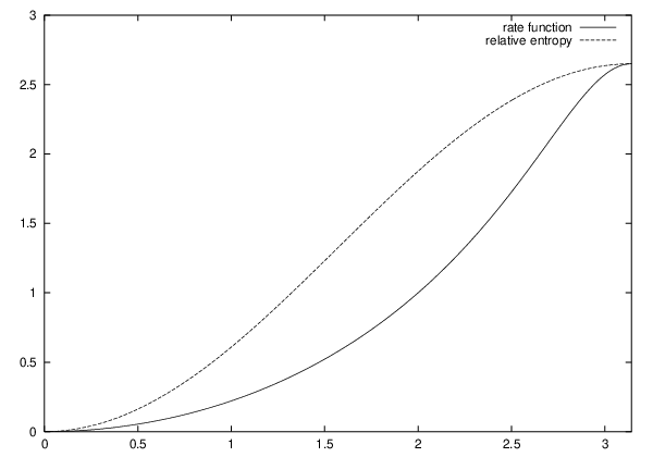
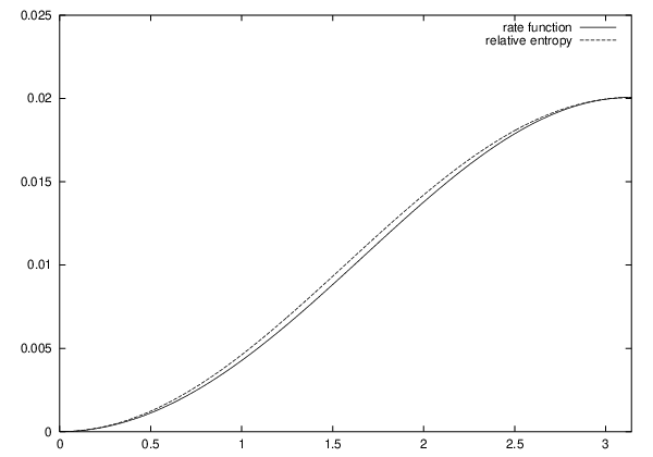
The proof will be given in Section 5.2; cf also [20]. It is easy to check numerically that I^​(ρ,σ)\hat{I}(\rho,\sigma) and S⁡(ρ,σ)S(\rho,\sigma) do not coincide in general. If we consider in particular the qubit case (d=2d=2) and express the density operators ρ,σ\rho,\sigma in Bloch form, i.e.

ρ=12​[1​I+x→⋅σ→],σ=12​[1​I+y→⋅σ→]\rho=\frac{1}{2}\bigl[{{\rm 1\mkern-4.8muI}}+\vec{x}\cdot\vec{\sigma}\bigr],\ \sigma=\frac{1}{2}\bigl[{{\rm 1\mkern-4.8muI}}+\vec{y}\cdot\vec{\sigma}\bigr] (28)

(where σ→=(σ1,σ2,σ3)\vec{\sigma}=(\sigma_{1},\sigma_{2},\sigma_{3}) are the Pauli matrices and x→,y→∈ℝ3\vec{x},\vec{y}\in\mathbb{R}^{3} with |x→|,|y→|≤1|\vec{x}|,|\vec{y}|\leq 1), we get for the rate function II from Equation (26)

I^​(ρ,σ)=−S⁡(σ)−|y→|​ln⁡[1+|x→|​cos⁡θ2]−1−|y→|2​ln⁡[1−|x→|24],\hat{I}(\rho,\sigma)=-S(\sigma)-|\vec{y}|\ln\left[\frac{1+|\vec{x}|\cos\theta}{2}\right]-\frac{1-|\vec{y}|}{2}\ln\left[\frac{1-|\vec{x}|^{2}}{4}\right], (29)

where θ\theta denotes the angle between x→\vec{x} and y→\vec{y} and S⁡(σ)S(\sigma) is the von Neumann entropy of σ\sigma. The relative entropy of σ\sigma and ρ\rho becomes [9]

S⁡(ρ,σ)=−S⁡(σ)−12​ln⁡(1+|x→|2)−|y→|​cos⁡(θ)2​ln⁡(1+|x→|1−|x→|).S(\rho,\sigma)=-S(\sigma)-\frac{1}{2}\ln(1+|\vec{x}|^{2})-\frac{|\vec{y}|\cos(\theta)}{2}\ln\left(\frac{1+|\vec{x}|}{1-|\vec{x}|}\right). (30)

We have plotted both quantities as functions of θ\theta for two different values of |x→|=|y→||\vec{x}|=|\vec{y}| in Figure 1, which shows that I⁡(ρ,σ)I(\rho,\sigma) is in general strictly smaller than S⁡(ρ,σ)S(\rho,\sigma).

Refer to caption
Refer to caption
Figure 1: Relative entropy and rate function I^\hat{I} as a function of the angle θ\theta between the two Bloch vectors x→\vec{x} and y→\vec{y}. The upper plot corresponds to the case |x→|=|y→|=0.9|\vec{x}|=|\vec{y}|=0.9 and the lower to |x→|=|y→|=0.1|\vec{x}|=|\vec{y}|=0.1.

3.3 Optimal rate functions

Hence, for a general input state ρ\rho we only know for sure that the optimal rate functions defined in Equation (12) and (13) have to satisfy (with p=Idp=\operatorname{Id} for full estimation)

I^≤ℐIdc,ℐId0≤ℐId≤S.\hat{I}\leq\mathcal{I}_{\operatorname{Id}}^{c},\mathcal{I}_{\operatorname{Id}}^{0}\leq\mathcal{I}_{\operatorname{Id}}\leq S. (31)

This is, however, not as bad as it looks like at a first glance: Since S⁡(ρ,σ)S(\rho,\sigma) and I^​(ρ,σ)\hat{I}(\rho,\sigma) coincide if ρ\rho and σ\sigma commute, we get

I^​(ρ,σ)=ℐIdc​(ρ,σ)=ℐId0​(ρ,σ)=ℐId​(ρ,σ)=S⁡(ρ,σ)=∑j=1dsj​(σ)​(ln⁡sj​(σ)−ln⁡sj​(ρ))∀ρ,σ∈𝒮​with​[ρ,σ]=0.\hat{I}(\rho,\sigma)=\mathcal{I}_{\operatorname{Id}}^{c}(\rho,\sigma)=\mathcal{I}_{\operatorname{Id}}^{0}(\rho,\sigma)=\mathcal{I}_{\operatorname{Id}}(\rho,\sigma)=S(\rho,\sigma)=\\ \sum_{j=1}^{d}s_{j}(\sigma)\,\bigl(\ln s_{j}(\sigma)-\ln s_{j}(\rho)\bigr)\quad\forall\rho,\sigma\in\mathcal{S}\ \text{with}\ [\rho,\sigma]=0. (32)

A second partial result arises if the input state is pure. In Proposition 5.5 we will show

ℐIdc​(ρ,σ)=I^​(ρ,σ)∀ρ,σ∈𝒮​with ρ pure,\mathcal{I}^{c}_{\operatorname{Id}}(\rho,\sigma)=\hat{I}(\rho,\sigma)\quad\forall\rho,\sigma\in\mathcal{S}\ \text{with $\rho$ pure}, (33)

and in Section 4.4 we will give some heuristic arguments which indicate that I^\hat{I} and ℐc\mathcal{I}^{c} coincide even for general input states. This indicates that (E^N)N∈ℕ(\hat{E}_{N})_{N\in\mathbb{N}} is the best scheme as long as we are insisting on some additional regularity conditions of the rate function – in the case at hand this is covariance. It is not clear, however, whether covariance can be replaced by something more general without breaking the equality with I^\hat{I}. There are at least some indications (cf. Section 5.3) that Equation (33) would still hold if we replace ℐIdc\mathcal{I}^{c}_{\operatorname{Id}} with ℐId0\mathcal{I}^{0}_{\operatorname{Id}}. Note that I^∈ℰ0​(p)\hat{I}\in\mathcal{E}^{0}(p) hence (33) already implies ℐ0​(ρ,σ)≥ℐc​(ρ,σ)\mathcal{I}^{0}(\rho,\sigma)\geq\mathcal{I}^{c}(\rho,\sigma) for pure ρ\rho. Our conjecture here is that equality holds for all ρ\rho and σ\sigma.

Another result which can be derived easily from Equation (33) and Proposition 4.9 is 𝒮∉ℰ⁡(Id)\mathcal{S}\not\in\mathcal{E}(\operatorname{Id}), i.e. there is no estimation scheme with relative entropy as its rate function. This follows from the fact that SS is lower semicontinuous and U⁡(d)\operatorname{U}(d)-invariant in the sense of Equation (11). Hence S∈ℰ⁡(Id)S\in\mathcal{E}(\operatorname{Id}) would imply according to Proposition 4.9 S∈ℰc​(Id)S\in\mathcal{E}^{c}(\operatorname{Id}) in contradiction to Equation (33) and the fact that S​(ρ,σ)>I^​(ρ,σ)S(\rho,\sigma)>\hat{I}(\rho,\sigma) holds for all pure states ρ,σ\rho,\sigma with ρ≠σ\rho\neq\sigma and ρ​σ≠0\rho\sigma\neq 0. On the other hand there is strong evidence that ℐId=S\mathcal{I}_{\operatorname{Id}}=S holds, i.e. that SS is the best upper bound of the set of all admissible rate functions. This would imply that we can find for each pair ρ0,σ0∈𝒮\rho_{0},\sigma_{0}\in\mathcal{S} an I∈ℰ⁡(Id)I\in\mathcal{E}(\operatorname{Id}) such that I⁡(ρ0,σ0)=S⁡(ρ0,σ0)I(\rho_{0},\sigma_{0})=S(\rho_{0},\sigma_{0}) holds, but II is much smaller than SS (most probably even smaller than I^\hat{I}) almost everywhere else. In Section 5.3 we will discuss these topics in greater detail. For now, let us summarize all our conjectures in the following Equation

I^=ℐIdc=ℐId0≤ℐ=S.\hat{I}=\mathcal{I}^{c}_{\operatorname{Id}}=\mathcal{I}^{0}_{\operatorname{Id}}\leq\mathcal{I}=S. (34)

4 Covariant observables

The aim of this section is to study estimation schemes which are U⁡(d)\operatorname{U}(d) covariant and permutation invariant, i.e. they do not prefer a special copy of the input state or a particular direction in the Hilbert space ℋ\mathcal{H}. Among a proof of Theorem 3.2 we will provide several general results, which are useful within the discussion of the questions raised in Section 3.3. Therefore only full estimation schemes are considered in this section (i.e. p=Idp=\operatorname{Id}), but most of the results in Subsection 4.2 and 4.3 can be generalized quite easily to pp-estimation schemes, if pp is sufficiently covariant.

4.1 Continuity properties

Let us start with some technical results concerning continuity and uniform convergence with respect to the original density matrix ρ\rho. They will become crucial within the discussion of group averages in the next section. Some of them, however, are quite interesting in their own right, and it is therefore reasonable to devote a whole subsection for them.

Central subjects of this discussion will be integrals of the form

hN​(ρ,f)=−1N​ln​∫𝒮e−N​f​(σ)​tr⁡(ρ⊗N​EN​(𝑑σ)),h_{N}(\rho,f)=\frac{-1}{N}\ln\int_{\mathcal{S}}e^{-Nf(\sigma)}\operatorname{tr}\bigl(\rho^{\otimes N}E_{N}(d\sigma)\bigr), (35)

where ff denotes an arbitrary, real valued function on 𝒮\mathcal{S}. Quantities of this form usually appear in Varadhan’s Theorem (cf. Theorem A.3), i.e. if the estimation scheme (EN)N∈ℕ(E_{N})_{N\in\mathbb{N}} satisfies the LDP with rate function II we have

limN→∞hN​(ρ,f)=h⁡(ρ,f)=infσ∈𝒮(I⁡(ρ,σ)+f⁡(σ)).\lim_{N\to\infty}h_{N}(\rho,f)=h(\rho,f)=\inf_{\sigma\in\mathcal{S}}\bigl(I(\rho,\sigma)+f(\sigma)\bigr). (36)

If on the other hand (EN)N∈ℕ(E_{N})_{N\in\mathbb{N}} does not necessarily satisfy the LDP but (36) holds for each ff and a density matrix ρ\rho, the sequence of probability measures tr⁡(ρ⊗N​EN​(⋅))\operatorname{tr}\bigl(\rho^{\otimes N}E_{N}(\,\cdot\,)\bigr) satisfies the Laplace principle (Definition A.4) which is equivalent to the large deviation principle (Theorem A.5). Hence the study of convergence properties of the hN​(ρ,f)h_{N}(\rho,f) is a useful tool to prove that the LDP holds for a given estimation scheme.

In this section we will discuss continuity of hh with respect to ρ\rho and uniformity of the convergence hN→hh_{N}\to h (again with respect to ρ\rho). The most crucial step in this direction is the following lemma.

Lemma 4.1

Consider an estimation scheme (EN)N∈ℕ(E_{N})_{N\in\mathbb{N}} satisfying the LDP with rate function II, an arbitrary continuous (real valued) function ff and the functionals hN,hh_{N},h defined in Equations (35) and (36).

  1. 1.

    For each non-degenerate density matrix ρ∈𝒮\rho\in\mathcal{S} and each sequence ℕ∋N↦ρN∈𝒮\mathbb{N}\ni N\mapsto\rho_{N}\in\mathcal{S} converging to ρ\rho we have

    limN→∞hN​(ρN,f)=limN→∞hN​(ρ,f)=h⁡(ρ,f)\lim_{N\to\infty}h_{N}(\rho_{N},f)=\lim_{N\to\infty}h_{N}(\rho,f)=h(\rho,f) (37)
  2. 2.

    If II is lower semicontinuous in both arguments, the lower bound

    lim infN→∞hN​(ρN,f)≥h⁡(ρ,f)\liminf_{N\to\infty}h_{N}(\rho_{N},f)\geq h(\rho,f) (38)

    holds even for degenerate ρ\rho.

Proof. Let us consider part 1 first. In this case the proof mainly depends on the following lemma which allows us to represent one sequence as a convex combination of two others.

Lemma 4.2

Consider two sequences ℕ∋N↦ρN(j)∈𝒮\mathbb{N}\ni N\mapsto\rho_{N}^{(j)}\in\mathcal{S}, j=1,2j=1,2 both converging to the same non-degenerate density matrix ρ∈𝒮\rho\in\mathcal{S}. For each λ∈ℝ\lambda\in\mathbb{R} with 0<λ<10<\lambda<1 there exists an integer Nλ∈ℕN_{\lambda}\in\mathbb{N} and a third sequence ℕ∋N↦σN∈𝒮\mathbb{N}\ni N\mapsto\sigma_{N}\in\mathcal{S} such that

ρN(1)=λ​ρN(2)+(1−λ)​σN∀N>ℕλ\rho_{N}^{(1)}=\lambda\rho_{N}^{(2)}+(1-\lambda)\sigma_{N}\quad\forall N>\mathbb{N}_{\lambda} (39)

holds.

Proof. Let κ=inf‖ϕ‖=1⟨ϕ,ρ​ϕ⟩\kappa=\inf_{\|\phi\|=1}\langle\phi,\rho\phi\rangle and define

ϵ=(1−λ)​κλ+1.\epsilon=\frac{(1-\lambda)\kappa}{\lambda+1}. (40)

Since ρ\rho is non-degenerate, we have κ>0\kappa>0 and therefore ϵ>0\epsilon>0 as well. Hence there is an Nλ∈ℕN_{\lambda}\in\mathbb{N} such that (with ϕ∈ℋ\phi\in\mathcal{H} and A∈ℬ⁡(ℋ)A\in\mathcal{B}(\mathcal{H}))

sup‖ϕ‖=1|⟨ϕ,(ρN(j)−ρ)​ϕ⟩|\displaystyle\sup_{\|\phi\|=1}|\langle\phi,(\rho_{N}^{(j)}-\rho)\phi\rangle| ≤sup‖A‖=1|tr⁡((ρN(j)−ρ)​A)|\displaystyle\leq\sup_{\|A\|=1}\bigl|\operatorname{tr}\bigl((\rho_{N}^{(j)}-\rho)A\bigr)\bigr| (41)
=‖ρN(j)−ρ‖1<ϵ\displaystyle=\|\rho_{N}^{(j)}-\rho\|_{1}<\epsilon (42)

holds for all N>NλN>N_{\lambda} and for j=1,2j=1,2. In addition we see by the triangle inequality that

sup‖ϕ‖=1|⟨ϕ,(ρN(1)−ρN(2))​ϕ⟩|<2​ϵ\sup_{\|\phi\|=1}|\langle\phi,(\rho_{N}^{(1)}-\rho_{N}^{(2)})\phi\rangle|<2\epsilon (43)

holds as well for all N>NλN>N_{\lambda}. Now define

δ=κ2​ϵ−12=λ1−λ\delta=\frac{\kappa}{2\epsilon}-\frac{1}{2}=\frac{\lambda}{1-\lambda} (44)

(the second equality follows from Equation (40)) and

σN=−δ​ρN(2)+(1+δ)​ρN(1)​for​N>Nλ\sigma_{N}=-\delta\rho_{N}^{(2)}+(1+\delta)\rho_{N}^{(1)}\ \text{for}\ N>N_{\lambda} (45)

(and σN∈𝒮\sigma_{N}\in\mathcal{S} arbitrary otherwise). Obviously tr⁡(σN)=1\operatorname{tr}(\sigma_{N})=1 and

−λ1−λ​ρN(2)+11−λ​ρN(1)=σN.\frac{-\lambda}{1-\lambda}\rho_{N}^{(2)}+\frac{1}{1-\lambda}\rho_{N}^{(1)}=\sigma_{N}. (46)

Hence

ρN(1)=λ​ρN(2)+(1−λ)​σN∀N>Nλ\rho_{N}^{(1)}=\lambda\rho_{N}^{(2)}+(1-\lambda)\sigma_{N}\quad\forall N>N_{\lambda} (47)

as stated.

It only remains to show that σN≥0\sigma_{N}\geq 0 (and therefore σN∈𝒮\sigma_{N}\in\mathcal{S}) holds for all N>NλN>N_{\lambda}. This follows from

⟨ϕ,σN​ϕ⟩\displaystyle\langle\phi,\sigma_{N}\phi\rangle =−δ⁡⟨ϕ,ρN(2)​ϕ⟩+(1+δ)​⟨ϕ,ρN(1)​ϕ⟩\displaystyle=-\delta\langle\phi,\rho_{N}^{(2)}\phi\rangle+(1+\delta)\langle\phi,\rho_{N}^{(1)}\phi\rangle (48)
≥−2​δ​ϵ−δ⁡⟨ϕ,ρN(1)​ϕ⟩+(1+δ)​⟨ϕ,ρN(1)​ϕ⟩\displaystyle\geq-2\delta\epsilon-\delta\langle\phi,\rho_{N}^{(1)}\phi\rangle+(1+\delta)\langle\phi,\rho_{N}^{(1)}\phi\rangle (49)
=−2​δ​ϵ+⟨ϕ,ρN(1)​ϕ⟩≥−2​δ​ϵ+⟨ϕ,ρ​ϕ⟩−ϵ\displaystyle=-2\delta\epsilon+\langle\phi,\rho_{N}^{(1)}\phi\rangle\geq-2\delta\epsilon+\langle\phi,\rho\phi\rangle-\epsilon (50)
≥−2​δ​ϵ+κ−ϵ=−ϵ⁡(2​δ+1)+κ=0,\displaystyle\geq-2\delta\epsilon+\kappa-\epsilon=-\epsilon(2\delta+1)+\kappa=0, (51)

where we have used Equation (43) in (49), Equation (42) in (50) and the definition of δ\delta (44) in (51). □\Box

Now let us apply this lemma to ρN(1)=ρ\rho_{N}^{(1)}=\rho and ρN(2)=ρN\rho_{N}^{(2)}=\rho_{N} for all N∈ℕN\in\mathbb{N}. For each λ∈(0,1)\lambda\in(0,1) we get an Nλ∈ℕN_{\lambda}\in\mathbb{N} such that hN​(ρ,f)=hN​(λ​ρN+(1−λ)​σN,f)h_{N}(\rho,f)=h_{N}(\lambda\rho_{N}+(1-\lambda)\sigma_{N},f) holds for all N>NλN>N_{\lambda}. Hence

limN→∞hN​(ρ,f)=limN→∞hN​(λ​ρN+(1−λ)​σN,f).\lim_{N\to\infty}h_{N}(\rho,f)=\lim_{N\to\infty}h_{N}(\lambda\rho_{N}+(1-\lambda)\sigma_{N},f). (52)

Using the definition of hNh_{N} in (35) we get:

hN(λρN+(1−λ)σN,f)=−1Nln(λNe−N​hN​(ρN,f)+OPEN∑n=1NλN−n​(1−λ)n​∫𝒮e−N​f​(σ)​tr⁡(AN,n​EN​(dσ))),h_{N}(\lambda\rho_{N}+(1-\lambda)\sigma_{N},f)=\frac{-1}{N}\ln\left(\lambda^{N}e^{-Nh_{N}(\rho_{N},f)}+\phantom{\sum_{n=1}^{N}\int_{\mathcal{S}}}\right.\\ \left.\sum_{n=1}^{N}\lambda^{N-n}(1-\lambda)^{n}\int_{\mathcal{S}}e^{-Nf(\sigma)}\operatorname{tr}\bigl(A_{N,n}E_{N}(d\sigma)\bigr)\right), (53)

where AN,nA_{N,n} denotes the sum of all tensor products consisting of N−nN-n factors ρN\rho_{N} and nn factors σN\sigma_{N}. We can rewrite this expression as

hN​(λ​ρN+(1−λ)​σN,f)=−ln⁡λ+hN​(ρN,f)−1N​ln⁡(1+eN​hN​(ρN,f)​∑n=1N(1−λλ)n​∫𝒮e−N​f​(σ)​tr⁡(AN,n​EN​(dσ))).h_{N}(\lambda\rho_{N}+(1-\lambda)\sigma_{N},f)=-\ln\lambda+h_{N}(\rho_{N},f)\\ -\frac{1}{N}\ln\left(1+e^{Nh_{N}(\rho_{N},f)}\sum_{n=1}^{N}\left(\frac{1-\lambda}{\lambda}\right)^{n}\int_{\mathcal{S}}e^{-Nf(\sigma)}\operatorname{tr}\bigl(A_{N,n}E_{N}(d\sigma)\bigr)\right). (54)

Since ρN\rho_{N} and σN\sigma_{N} are density matrices, the operators AN,nA_{N,n} are positive. Hence, the argument of the last logarithm in Equation (54) is greater than one and the logarithm therefore positive. This implies:

hN​(ρN,f)≥hN​(λ​ρN+(1−λ)​σN,f)+ln⁡(λ),h_{N}(\rho_{N},f)\geq h_{N}(\lambda\rho_{N}+(1-\lambda)\sigma_{N},f)+\ln(\lambda), (55)

and with Equation (52)

lim infN→∞hN​(ρN,f)≥lim infN→∞hN​(λ​ρN+(1−λ)​σN,f)+ln⁡(λ)=limN→∞hN​(ρ,f)+ln⁡(λ).\liminf_{N\to\infty}h_{N}(\rho_{N},f)\geq\liminf_{N\to\infty}h_{N}(\lambda\rho_{N}+(1-\lambda)\sigma_{N},f)+\ln(\lambda)=\\ \lim_{N\to\infty}h_{N}(\rho,f)+\ln(\lambda). (56)

Since λ∈(0,1)\lambda\in(0,1) is arbitrary we get lim infN→∞hN​(ρN,f)≥limN→∞hN​(ρ,f)\liminf_{N\to\infty}h_{N}(\rho_{N},f)\geq\lim_{N\to\infty}h_{N}(\rho,f). The other inequality (i.e. lim supN→∞hN​(ρN,f)≤limN→∞hN​(ρ,f)\limsup_{N\to\infty}h_{N}(\rho_{N},f)\leq\lim_{N\to\infty}h_{N}(\rho,f)) can be derived with the same argument, if we exchange the role of ρ\rho and ρN\rho_{N} (i.e. apply Lemma 4.2 to ρN(1)=ρN\rho_{N}^{(1)}=\rho_{N} and ρN(2)=ρ\rho_{N}^{(2)}=\rho for all N∈ℕN\in\mathbb{N}). Hence limN→∞hN​(ρN,f)=limN→∞hN​(ρ,f)\lim_{N\to\infty}h_{N}(\rho_{N},f)=\lim_{N\to\infty}h_{N}(\rho,f) as stated. The equality limN→∞hN​(ρ,f)=h⁡(ρ,f)\lim_{N\to\infty}h_{N}(\rho,f)=h(\rho,f) follows from Varadhan’s Theorem (Theorem A.3).

Now consider statement 2. If ρ\rho is degenerate, the method used above can not be applied. However, if the rate function II is sufficiently continuous, we can extend (parts of) the result derived for non-degenerate density matrices to the degenerate case. To this end we need the following lemma:

Lemma 4.3

Consider a compact metric space (X,d)(X,d) and a lower semicontinuous function F:X×X→[c,∞]F:X\times X\to[c,\infty], c∈ℝc\in\mathbb{R}. The infimum F¯​(x)=infy∈XF⁡(x,y)\underline{F}(x)=\inf_{y\in X}F(x,y) is lower semicontinuous as well.

Proof. Due to lower semicontinuity of FF, we find for each (x,y)∈X×X(x,y)\in X\times X and each ϵ>0\epsilon>0 a δx,y>0\delta_{x,y}>0 with

d⁡(x,x′)<δx,y,d⁡(y,y′)<δx,y⇒F⁡(x′,y′)>F⁡(x,y)−ϵ.d(x,x^{\prime})<\delta_{x,y},\ d(y,y^{\prime})<\delta_{x,y}\Rightarrow F(x^{\prime},y^{\prime})>F(x,y)-\epsilon. (57)

Since XX is compact, each fixed x∈Xx\in X admits finitely many points y1,…,yk∈Xy_{1},\ldots,y_{k}\in X such that the neighborhoods Uj={y′∈X|d⁡(y′,yj)<δx,yj}U_{j}=\{y^{\prime}\in X\,|\,d(y^{\prime},y_{j})<\delta_{x,y_{j}}\} overlap XX. Now define δ=minj⁡δx,yj>0\delta=\min_{j}\delta_{x,y_{j}}>0. For each x′x^{\prime} satisfying d⁡(x,x′)<δd(x,x^{\prime})<\delta and each y′∈Xy^{\prime}\in X there is a j=1,…,kj=1,\ldots,k with F⁡(x′,y′)>F⁡(x,yj)−ϵF(x^{\prime},y^{\prime})>F(x,y_{j})-\epsilon. Hence F⁡(x′,y′)>infyF⁡(x,y)−ϵF(x^{\prime},y^{\prime})>\inf_{y}F(x,y)-\epsilon and we get

d⁡(x,x′)<δ⇒F¯​(x′)=infy′F⁡(x′,y′)>infyF⁡(x,y)−ϵ.d(x,x^{\prime})<\delta\Rightarrow\underline{F}(x^{\prime})=\inf_{y^{\prime}}F(x^{\prime},y^{\prime})>\inf_{y}F(x,y)-\epsilon. (58)

Since δ>0\delta>0 this shows that F¯\underline{F} is lower semicontinuous at xx and since xx is arbitrary the statement follows. □\Box

Let us apply this lemma to F⁡(ρ,σ)=I⁡(ρ,σ)+f⁡(σ)F(\rho,\sigma)=I(\rho,\sigma)+f(\sigma). Since II is lower semicontinuous by assumption we get for each ϵ>0\epsilon>0 a δ>0\delta>0 such that ‖ρ′−ρ‖1<δ\|\rho^{\prime}-\rho\|_{1}<\delta implies h⁡(ρ′,f)>h⁡(ρ,f)−ϵh(\rho^{\prime},f)>h(\rho,f)-\epsilon. Together with the convexity of the δ\delta-ball around ρ\rho this implies

h⁡(λ​ρ+(1−λ)​ρ′,f)>h⁡(ρ,f)−ϵ∀λ∈(0,1).h(\lambda\rho+(1-\lambda)\rho^{\prime},f)>h(\rho,f)-\epsilon\quad\forall\lambda\in(0,1). (59)

If (ρN)N∈ℕ(\rho_{N})_{N\in\mathbb{N}} is a sequence in 𝒮\mathcal{S} converging to ρ\rho, the convex linear combinations λ​ρN+(1−λ)​ρ′\lambda\rho_{N}+(1-\lambda)\rho^{\prime} converges to λ​ρ+(1−λ)​ρ′\lambda\rho+(1-\lambda)\rho^{\prime}. As in Equation (56) we get

lim infN→∞hN​(λ​ρN+(1−λ)​ρ′,f)≤lim infN→∞hN​(ρN,f)−ln⁡(λ).\liminf_{N\to\infty}h_{N}(\lambda\rho_{N}+(1-\lambda)\rho^{\prime},f)\leq\liminf_{N\to\infty}h_{N}(\rho_{N},f)-\ln(\lambda). (60)

Now assume without loss of generality that ρ′\rho^{\prime} is non-degenerate. Then λ​ρ+(1−λ)​ρ′\lambda\rho+(1-\lambda)\rho^{\prime} is non-degenerate as well and we have according to item 1

lim infN→∞hN​(λ​ρN+(1−λ)​ρ′,f)=h⁡(λ​ρ+(1−λ)​ρ′,f)>h⁡(ρ,f)−ϵ.\liminf_{N\to\infty}h_{N}(\lambda\rho_{N}+(1-\lambda)\rho^{\prime},f)=h(\lambda\rho+(1-\lambda)\rho^{\prime},f)>h(\rho,f)-\epsilon. (61)

Hence

lim infN→∞hN​(ρN,f)≥h⁡(ρ,f)−ϵ+ln⁡(λ).\liminf_{N\to\infty}h_{N}(\rho_{N},f)\geq h(\rho,f)-\epsilon+\ln(\lambda). (62)

Since ϵ>0\epsilon>0 and λ∈(0,1)\lambda\in(0,1) are arbitrary the statement follows. □\Box

According to Proposition 1.2.7 of [13] this lemma implies immediately that the convergence hN→hh_{N}\to h is uniform on each compact set of non-degenerate density matrices.

Proposition 4.4

Consider the same assumptions as in the preceding lemma and a compact set K⊂𝒮K\subset\mathcal{S} consisting only of non-degenerate density matrices. Then the convergence hN→hh_{N}\to h is uniform on KK, i.e.

limN→∞s​u​pρ∈K​|hN​(ρ,f)−h⁡(ρ,f)|=0\lim_{N\to\infty}sup_{\rho\in K}\left|h_{N}(\rho,f)-h(\rho,f)\right|=0 (63)

holds.

Another simple consequence of Lemma 4.1 is the continuity of h⁡(⋅,f)h(\,\cdot\,,f) on the interior of 𝒮\mathcal{S}. The proof is again omitted, since it can be taken without change from [13] (first paragraph of the proof of Proposition 1.2.7).

Proposition 4.5

Consider again the assumptions from Lemma 4.1. The function 𝒮∋ρ↦h⁡(ρ,f)∈ℝ\mathcal{S}\ni\rho\mapsto h(\rho,f)\in\mathbb{R} is continuous at each non-degenerate ρ\rho.

This is a somewhat surprising result, because it is derived without any further assumption on the rate function II. Although it does not imply that I⁡(ρ,σ)I(\rho,\sigma) is continuous in ρ\rho, it shows at least that the dependence of II on the original density matrix ρ\rho is quite regular on the interior of the state space 𝒮\mathcal{S}. On the boundary, however, nothing can be said. The discussion in Sections 5.3 and 5.4 will indicate that this is probably a fundamental aspect of admissible rate functions and not just a problem of the methods used in the proofs.

Let us consider now the natural action of U⁡(d)\operatorname{U}(d) on the set 𝒞⁡(𝒮)\mathcal{C}(\mathcal{S}) of continuous functions on 𝒮\mathcal{S}, i.e. for each U∈U⁡(d)U\in\operatorname{U}(d) and each f∈𝒞⁡(𝒮)f\in\mathcal{C}(\mathcal{S}) define αU​f∈𝒞⁡(𝒮)\alpha_{U}f\in\mathcal{C}(\mathcal{S}) by

αU​f​(σ)=f⁡(U​σ​U∗).\alpha_{U}f(\sigma)=f(U\sigma U^{*}). (64)

Then we can consider for each fixed ρ∈𝒮\rho\in\mathcal{S} and each ff the functions

U⁡(d)∋U↦hN​(U∗​ρ​U,αU​f)∈ℝ​and​U⁡(d)∋U↦h⁡(U∗​ρ​U,αU​f)∈ℝ,\operatorname{U}(d)\ni U\mapsto h_{N}(U^{*}\rho U,\alpha_{U}f)\in\mathbb{R}\ \text{and}\ \operatorname{U}(d)\ni U\mapsto h(U^{*}\rho U,\alpha_{U}f)\in\mathbb{R}, (65)

and pose the same question as above – but now considering the dependency on UU rather than on ρ\rho. The following is the analog of Lemma 4.1.

Lemma 4.6

Consider an estimation scheme (EN)N∈ℕ(E_{N})_{N\in\mathbb{N}} satisfying the LDP with rate function II, an arbitrary continuous (real valued) function ff and the functionals hN,hh_{N},h defined in Equations (35) and (36).

  1. 1.

    For each non-degenerate density matrix ρ∈𝒮\rho\in\mathcal{S} and each sequence ℕ∋N↦UN∈U⁡(d)\mathbb{N}\ni N\mapsto U_{N}\in\operatorname{U}(d) converging to U∈U⁡(d)U\in\operatorname{U}(d) we have

    limN→∞hN​(UN∗​ρ​UN,αUN​f)=limN→∞hN​(U∗​ρ​U,αU​f)=h⁡(U∗​ρ​U,αU​f)\lim_{N\to\infty}h_{N}(U_{N}^{*}\rho U_{N},\alpha_{U_{N}}f)=\lim_{N\to\infty}h_{N}(U^{*}\rho U,\alpha_{U}f)=h(U^{*}\rho U,\alpha_{U}f) (66)
  2. 2.

    If II is lower semicontinuous in both arguments, the lower bound

    lim infN→∞hN​(UN∗​ρ​UN,αUN​f)≥h⁡(U∗​ρ​U,αU​f)\liminf_{N\to\infty}h_{N}(U_{N}^{*}\rho U_{N},\alpha_{U_{N}}f)\geq h(U^{*}\rho U,\alpha_{U}f) (67)

    holds even for degenerate ρ\rho.

Proof. To prove item 1 let us start with the observation that the function sequence (αUM​f)M∈ℕ(\alpha_{U_{M}}f)_{M\in\mathbb{N}} converges uniformly to αU​f\alpha_{U}f: Due to compactness of 𝒮\mathcal{S} the function ff is not just continuous but even uniformly continuous, i.e. for each ϵ>0\epsilon>0 there is a δ>0\delta>0 with

‖σ1−σ2‖1<δ⇒|f⁡(σ1)−f⁡(σ2)|<ϵ.\|\sigma_{1}-\sigma_{2}\|_{1}<\delta\Rightarrow|f(\sigma_{1})-f(\sigma_{2})|<\epsilon. (68)

Convergence of (UM)M∈ℕ(U_{M})_{M\in\mathbb{N}} implies the existence of Mϵ∈ℕM_{\epsilon}\in\mathbb{N} with M>MϵM>M_{\epsilon} ⇒\Rightarrow ‖UM−U‖<δ/2\|U_{M}-U\|<\delta/2. For each σ\sigma and each M>MϵM>M_{\epsilon} we therefore get

‖UM​σ​UM∗−U​σ​U∗‖1\displaystyle\|U_{M}\sigma U_{M}^{*}-U\sigma U^{*}\|_{1} ≤‖UM​σ​UM∗−UM​σ​U∗‖1+‖UM​σ​U∗−U​σ​U∗‖1\displaystyle\leq\|U_{M}\sigma U_{M}^{*}-U_{M}\sigma U^{*}\|_{1}+\|U_{M}\sigma U^{*}-U\sigma U^{*}\|_{1} (69)
≤‖UM∗−U∗‖​‖UM‖​‖σ‖1+‖UM−U‖|U∗|‖σ‖1<δ,\displaystyle\leq\|U_{M}^{*}-U^{*}\|\|U_{M}\|\|\sigma\|_{1}+\|U_{M}-U\|\|U^{*}\|\|\sigma\|_{1}<\delta, (70)

which implies together with (68) for an arbitrary σ\sigma and M>MϵM>M_{\epsilon}

|αUM​f​(σ)−αU​f​(σ)|=|f⁡(UM​σ​UM∗)−f⁡(U​σ​U∗)|<ϵ.|\alpha_{U_{M}}f(\sigma)-\alpha_{U}f(\sigma)|=|f(U_{M}\sigma U_{M}^{*})-f(U\sigma U^{*})|<\epsilon. (71)

In other words the convergence αUM​f→αU​f\alpha_{U_{M}}f\to\alpha_{U}f is uniform as stated (since MϵM_{\epsilon} does not depend on σ\sigma).

To proceed, it is necessary to consider the following simple properties of the functionals hNh_{N} and hh: If f,f1f,f_{1} denotes continuous functions on 𝒮\mathcal{S} and ϵ∈ℝ\epsilon\in\mathbb{R} we have for all ρ\rho

f≥f1⇒hN​(ρ,f)≥hN​(ρ,f1),and​hN​(ρ,f+ϵ)=hN​(ρ,f)+ϵ,f\geq f_{1}\Rightarrow h_{N}(\rho,f)\geq h_{N}(\rho,f_{1}),\ \text{and}\ h_{N}(\rho,f+\epsilon)=h_{N}(\rho,f)+\epsilon, (72)

and from Lemma 4.1 we already know that for all ϵ>0\epsilon>0 and all ff there is an N⁡[ϵ,f]∈ℕN[\epsilon,f]\in\mathbb{N} with

N>N⁡[ϵ,f]⇒|hN​(UN∗​ρ​UN,f)−h⁡(U∗​ρ​U,f)|<ϵ.N>N[\epsilon,f]\Rightarrow|h_{N}(U_{N}^{*}\rho U_{N},f)-h(U^{*}\rho U,f)|<\epsilon. (73)

Uniform convergence αUM​f→αU​f\alpha_{U_{M}}f\to\alpha_{U}f implies that αU​f−ϵ≤αUM​f≤αU​f+ϵ\alpha_{U}f-\epsilon\leq\alpha_{U_{M}}f\leq\alpha_{U}f+\epsilon holds for all M>MϵM>M_{\epsilon}. Hence for all N∈ℕN\in\mathbb{N} we have

hN​(UN∗​ρ​UN,αU​f)−ϵ≤hN​(UN∗​ρ​UN,αUM​f)≤hN​(UN∗​ρ​UN,αU​f)+ϵh_{N}(U_{N}^{*}\rho U_{N},\alpha_{U}f)-\epsilon\leq h_{N}(U_{N}^{*}\rho U_{N},\alpha_{U_{M}}f)\leq h_{N}(U_{N}^{*}\rho U_{N},\alpha_{U}f)+\epsilon (74)

according to (72). Together with (73) we get

N>N⁡[ϵ,αU​f],M>Mϵ⇒|hN​(UN∗​ρ​UN,αUM​f)−h⁡(U∗​ρ​U,αU​f)|<2​ϵ,N>N[\epsilon,\alpha_{U}f],\ M>M_{\epsilon}\Rightarrow|h_{N}(U_{N}^{*}\rho U_{N},\alpha_{U_{M}}f)-h(U^{*}\rho U,\alpha_{U}f)|<2\epsilon, (75)

which implies Equation (66).

Statement 2 can be shown in the same way, if we replace Equation (73) by (cf. Lemma 4.1)

N>N⁡[ϵ,f]⇒hN​(UN∗​ρ​UN,f)≥h⁡(U∗​ρ​U,f)−ϵN>N[\epsilon,f]\Rightarrow h_{N}(U_{N}^{*}\rho U_{N},f)\geq h(U^{*}\rho U,f)-\epsilon (76)

and use only the lower bound of (74). □\Box

As in the case of Lemma 4.1 we can now derive continuity and uniformity properties from this result. The following proposition is (again) an immediate consequence of [13, Prop. 1.2.7]. The proof is therefore omitted.

Proposition 4.7

Consider the same assumptions as in Lemma 4.6 and a non-degenerate density matrix ρ\rho.

  1. 1.

    The function

    U⁡(d)∋U↦h⁡(U∗​ρ​U,αU​f)=infσ∈𝒮(I⁡(U∗​ρ​U,U∗​σ​U)+f⁡(σ))∈ℝ\operatorname{U}(d)\ni U\mapsto h(U^{*}\rho U,\alpha_{U}f)=\inf_{\sigma\in\mathcal{S}}\bigl(I(U^{*}\rho U,U^{*}\sigma U)+f(\sigma)\bigr)\in\mathbb{R} (77)

    is continuous.

  2. 2.

    The convergence of hN​(U∗​ρ​U,αU​f)h_{N}(U^{*}\rho U,\alpha_{U}f) to h⁡(U∗​ρ​U,αU​f)h(U^{*}\rho U,\alpha_{U}f) is uniform in UU, i.e.

    limN→∞supU∈U⁡(d)|hN​(U∗​ρ​U,αU​f)−h⁡(U∗​ρ​U,αU​f)|=0\lim_{N\to\infty}\sup_{U\in\operatorname{U}(d)}|h_{N}(U^{*}\rho U,\alpha_{U}f)-h(U^{*}\rho U,\alpha_{U}f)|=0 (78)

    holds.

4.2 Averaging

Let us consider now the question whether covariance and permutation invariance are “harmful” for the rate function; i.e. can we hope to exhaust the optimal upper bounds from Equation (12) with schemes admitting these symmetry properties? One possible way to answer this question is to start with a general scheme (EN)N∈ℕ(E_{N})_{N\in\mathbb{N}} and to average over the unitary and the permutation group. For the latter this leads to

E¯N​(Δ)=1N!​∑p∈SNVp​EN​(Δ)​Vp∗,\overline{E}_{N}(\Delta)=\frac{1}{N!}\sum_{p\in\operatorname{S}_{N}}V_{p}E_{N}(\Delta)V_{p}^{*}, (79)

and since we have

tr⁡(ρ⊗N​Vp​EN​(Δ)​Vp∗)=tr⁡(Vp∗​ρ⊗N​Vp​EN​(Δ))=tr⁡(ρ⊗N​EN​(Δ))\operatorname{tr}\bigl(\rho^{\otimes N}V_{p}E_{N}(\Delta)V_{p}^{*}\bigr)=\operatorname{tr}\bigl(V_{p}^{*}\rho^{\otimes N}V_{p}E_{N}(\Delta)\bigr)=\operatorname{tr}\bigl(\rho^{\otimes N}E_{N}(\Delta)\bigr) (80)

for each permutation p∈SNp\in\operatorname{S}_{N}, we see that the rate function is not changed at all by this procedure. Hence, for the rest of this section we can assume without loss of generality that each scheme is permutation invariant.

This leads us to averages over the unitary group, i.e.

E¯N(Δ)=∫U⁡(d)U⊗NEN(U∗ΔU)U⊗N∗dU.\overline{E}_{N}(\Delta)=\int_{\operatorname{U}(d)}U^{\otimes N}E_{N}(U^{*}\Delta U)U^{\otimes N*}dU. (81)

Here the situation is (unfortunately) different. The following proposition shows that the convergence behavior of E¯N\overline{E}_{N} is in general worse than that of ENE_{N}.

Proposition 4.8

Consider an estimation scheme (EN)N∈ℕ(E_{N})_{N\in\mathbb{N}} satisfying the LDP with rate function II and the corresponding averaged scheme (E¯N)N∈ℕ(\overline{E}_{N})_{N\in\mathbb{N}} from Equation (81). For each non-degenerate density matrix ρ\rho the sequence of probability measures tr⁡(ρ⊗N​E¯N​(⋅))\operatorname{tr}\bigl(\rho^{\otimes N}\overline{E}_{N}(\,\cdot\,)\bigr) satisfies the LDP with rate function I¯ρ\overline{I}_{\rho} given by

I¯ρ​(σ)=I¯​(ρ,σ)=infU∈U⁡(d)I⁡(U∗​ρ​U,U∗​σ​U).\overline{I}_{\rho}(\sigma)=\overline{I}(\rho,\sigma)=\inf_{U\in\operatorname{U}(d)}I(U^{*}\rho U,U^{*}\sigma U). (82)

Proof. It is sufficient to show that the measures tr⁡(ρ⊗N​E¯N​(⋅))\operatorname{tr}\bigl(\rho^{\otimes N}\overline{E}_{N}(\,\cdot\,)\bigr) satisfy the Laplace principle with the same rate function (cf. Theorem A.5), because the Laplace principle is equivalent to the large deviation principle. Hence we have to show that

limN→∞−1N​ln​∫𝒮e−N​f​(σ)​tr⁡(ρ⊗N​E¯N​(𝑑σ))=infσ∈𝒮(f⁡(σ)+I¯​(ρ,σ))\lim_{N\to\infty}\frac{-1}{N}\ln\int_{\mathcal{S}}e^{-Nf(\sigma)}\operatorname{tr}\bigl(\rho^{\otimes N}\overline{E}_{N}(d\sigma)\bigr)=\inf_{\sigma\in\mathcal{S}}\bigl(f(\sigma)+\overline{I}(\rho,\sigma)\bigr) (83)

holds for all continuous functions ff on 𝒮\mathcal{S}. Inserting the definition of E¯N\overline{E}_{N} we get

∫𝒮e−N​f​(σ)​tr⁡(ρ⊗N​E¯N​(𝑑σ))=∫U⁡(d)∫𝒮e−N​f​(U​σ​U∗)​tr⁡((U∗​ρ​U)⊗N​EN​(dσ))​dU,\int_{\mathcal{S}}e^{-Nf(\sigma)}\operatorname{tr}\bigl(\rho^{\otimes N}\overline{E}_{N}(d\sigma)\bigr)\\ =\int_{\operatorname{U}(d)}\int_{\mathcal{S}}e^{-Nf(U\sigma U^{*})}\operatorname{tr}\bigl((U^{*}\rho U)^{\otimes N}E_{N}(d\sigma)\bigr)dU, (84)

or with the notation from Subsection 4.1 (cf. Equations (35) and (64))

∫𝒮e−N​f​(σ)​tr⁡(ρ⊗N​E¯N​(𝑑σ))=∫U⁡(d)e−N​hN​(U∗​ρ​U,αU​f)​𝑑U.\int_{\mathcal{S}}e^{-Nf(\sigma)}\operatorname{tr}\bigl(\rho^{\otimes N}\overline{E}_{N}(d\sigma)\bigr)=\int_{\operatorname{U}(d)}e^{-Nh_{N}(U^{*}\rho U,\alpha_{U}f)}dU. (85)

According to Proposition 4.7 the quantity hN​(U∗​ρ​U,αU​f)h_{N}(U^{*}\rho U,\alpha_{U}f) converges uniformly in UU to h⁡(U∗​ρ​U,αU​f)h(U^{*}\rho U,\alpha_{U}f), i.e. for each ϵ>0\epsilon>0 there is an Nϵ∈ℕN_{\epsilon}\in\mathbb{N} such that

N>Nϵ⇒h⁡(U∗​ρ​U,αU​f)+ϵ≥hN​(U∗​ρ​U,αU​f)≥h⁡(U∗​ρ​U,αU​f)−ϵ∀U∈U⁡(d)N>N_{\epsilon}\Rightarrow\\ h(U^{*}\rho U,\alpha_{U}f)+\epsilon\geq h_{N}(U^{*}\rho U,\alpha_{U}f)\geq h(U^{*}\rho U,\alpha_{U}f)-\epsilon\quad\forall U\in\operatorname{U}(d) (86)

holds. Hence, for each ϵ>0\epsilon>0 we get

lim supN→∞−1N​ln​∫U⁡(d)e−N⁡(h⁡(U∗​ρ​U,αU​f)+ϵ)​dU≥lim supN→∞−1N​ln​∫U⁡(d)e−N​hN​(U∗​ρ​U,αU​f)​dU.\limsup_{N\to\infty}\frac{-1}{N}\ln\int_{\operatorname{U}(d)}e^{-N(h(U^{*}\rho U,\alpha_{U}f)+\epsilon)}dU\geq\\ \limsup_{N\to\infty}\frac{-1}{N}\ln\int_{\operatorname{U}(d)}e^{-Nh_{N}(U^{*}\rho U,\alpha_{U}f)}dU. (87)

From Proposition 4.7 we know that h⁡(U∗​ρ​U,αU​f)h(U^{*}\rho U,\alpha_{U}f) is continuous in UU and we can apply Varadhan’s Theorem (Theorem A.3) to the left hand side of this inequality. Together with

infU∈U⁡(d)h⁡(U∗​ρ​U,αU​f)\displaystyle\inf_{U\in\operatorname{U}(d)}h(U^{*}\rho U,\alpha_{U}f) =infU∈U⁡(d)infσ∈𝒮(I⁡(U∗​ρ​U,σ)+f⁡(U​σ​U∗))\displaystyle=\inf_{U\in\operatorname{U}(d)}\inf_{\sigma\in\mathcal{S}}\bigl(I(U^{*}\rho U,\sigma)+f(U\sigma U^{*})\bigr) (88)
=infU∈U⁡(d)infσ∈𝒮(I⁡(U∗​ρ​U,U∗​σ​U)+f⁡(σ))\displaystyle=\inf_{U\in\operatorname{U}(d)}\inf_{\sigma\in\mathcal{S}}\bigl(I(U^{*}\rho U,U^{*}\sigma U)+f(\sigma)\bigr) (89)
=infσ∈𝒮(I¯​(ρ,σ)+f⁡(σ))\displaystyle=\inf_{\sigma\in\mathcal{S}}\bigl(\overline{I}(\rho,\sigma)+f(\sigma)\bigr) (90)

this implies the upper bound

lim supN→∞−1N​ln​∫U⁡(d)e−N​hN​(U∗​ρ​U,αU​f)​𝑑U≤infσ∈𝒮(I¯​(ρ,σ)+f⁡(σ))+ϵ.\limsup_{N\to\infty}\frac{-1}{N}\ln\int_{\operatorname{U}(d)}e^{-Nh_{N}(U^{*}\rho U,\alpha_{U}f)}dU\leq\inf_{\sigma\in\mathcal{S}}\bigl(\overline{I}(\rho,\sigma)+f(\sigma)\bigr)+\epsilon. (91)

The lower bound

lim infN→∞−1N​ln​∫U⁡(d)e−N​hN​(U∗​ρ​U,αU​f)​𝑑U≥infσ∈𝒮(I¯​(ρ,σ)+f⁡(σ))−ϵ\liminf_{N\to\infty}\frac{-1}{N}\ln\int_{\operatorname{U}(d)}e^{-Nh_{N}(U^{*}\rho U,\alpha_{U}f)}dU\geq\inf_{\sigma\in\mathcal{S}}\bigl(\overline{I}(\rho,\sigma)+f(\sigma)\bigr)-\epsilon (92)

can be shown in the same way. Since ϵ>0\epsilon>0 was arbitrary, Equation (83) follows from (85), (91) and (92), which concludes the proof. □\Box

Hence, the best we can hope is that the averaged scheme satisfies the LDP with rate function I¯\overline{I} which is actually the worst U⁡(d)\operatorname{U}(d)-invariant rate function which can be derived from II. Only if II is U⁡(d)\operatorname{U}(d) invariant itself (such that I¯=I\overline{I}=I holds), the convergence behavior of (E¯N)N∈ℕ(\overline{E}_{N})_{N\in\mathbb{N}} is as good as than that of (EN)N∈ℕ(E_{N})_{N\in\mathbb{N}}. The following proposition shows that at least in this case the convergence problems on the boundary of 𝒮\mathcal{S} can be solved.

Proposition 4.9

If (EN)N∈ℕ(E_{N})_{N\in\mathbb{N}} is an estimation scheme satisfying the LDP with a U⁡(d)\operatorname{U}(d)-invariant, lower semicontinuous (in both arguments) rate function II, the averaged scheme (E¯N)N∈ℕ(\overline{E}_{N})_{N\in\mathbb{N}} defined in Equation (81) satisfies the LDP with the same rate function.

Proof. We will show again the alternative statement that the sequence tr⁡(ρ⊗N​E¯N​(⋅))\operatorname{tr}\bigl(\rho^{\otimes N}\overline{E}_{N}(\,\cdot\,)\bigr) satisfies the Laplace principle, i.e. Equation (83) holds for all continuous real valued functions ff and with I¯\overline{I} replaced by II. As in the last proof we can rewrite this in terms of the functionals hNh_{N} and hh defined in Equation (35) and (36), i.e. we have to show that (cf. Equation (85))

lim supN→∞−1N​ln​∫U⁡(d)e−N​hN​(U∗​ρ​U,αU​f)​𝑑U≤h⁡(ρ,f)\limsup_{N\to\infty}\frac{-1}{N}\ln\int_{\operatorname{U}(d)}e^{-Nh_{N}(U^{*}\rho U,\alpha_{U}f)}dU\leq h(\rho,f) (93)

and

lim infN→∞−1N​ln​∫U⁡(d)e−N​hN​(U∗​ρ​U,αU​f)​𝑑U≥h⁡(ρ,f)\liminf_{N\to\infty}\frac{-1}{N}\ln\int_{\operatorname{U}(d)}e^{-Nh_{N}(U^{*}\rho U,\alpha_{U}f)}dU\geq h(\rho,f) (94)

hold. But now the convergence of hN​(U∗​ρ​U,αU​f)h_{N}(U^{*}\rho U,\alpha_{U}f) to h⁡(ρ,f)h(\rho,f) is only known to be pointwise (and not necessarily uniform) in UU. Therefore, we can not proceed as in Proposition 4.8. Instead we will use different strategies for the upper and the lower bound.

To get the upper bound note that ff is (as a continuous function on a compact set) bounded from above by a constant K>0K>0. Therefore the functions U↦hN​(U∗​ρ​U,αU​f)U\mapsto h_{N}(U^{*}\rho U,\alpha_{U}f) are bounded as well (by the same constant) and we get (note that h⁡(U∗​ρ​U,αU​f)=h⁡(ρ,f)h(U^{*}\rho U,\alpha_{U}f)=h(\rho,f) holds for all UU by assumption)

limN→∞∫U⁡(d)|hN​(U∗​ρ​U,αU​f)−h⁡(ρ,f)|​𝑑U=0.\lim_{N\to\infty}\int_{\operatorname{U}(d)}\bigl|h_{N}(U^{*}\rho U,\alpha_{U}f)-h(\rho,f)\bigr|dU=0. (95)

by the dominated convergence theorem. Now let us introduce for each ϵ>0\epsilon>0 and each N∈ℕN\in\mathbb{N} the set

ΔN,ϵ={U∈U⁡(d)||hN​(U∗​ρ​U,αU​f)−h⁡(ρ,f)|>ϵ}.\Delta_{N,\epsilon}=\{U\in\operatorname{U}(d)\,|\,\bigl|h_{N}(U^{*}\rho U,\alpha_{U}f)-h(\rho,f)\bigr|>\epsilon\}. (96)

From Equation (95) we see that for each δ>0\delta>0 there is an Nδ∈ℕN_{\delta}\in\mathbb{N} such that N>NδN>N_{\delta} implies

|ΔN,ϵ|​ϵ≤∫U⁡(d)|hN​(U∗​ρ​U,αU​f)−h⁡(ρ,f)|​𝑑U<δ,\left|\Delta_{N,\epsilon}\right|\epsilon\leq\int_{\operatorname{U}(d)}\bigl|h_{N}(U^{*}\rho U,\alpha_{U}f)-h(\rho,f)\bigr|dU<\delta, (97)

where |ΔN,ϵ|\left|\Delta_{N,\epsilon}\right| denotes the volume of ΔN,ϵ\Delta_{N,\epsilon} with respect to the Haar measure (note that ΔN,ϵ\Delta_{N,\epsilon} is due to continuity of U↦hN​(U∗​ρ​U,αU​f)U\mapsto h_{N}(U^{*}\rho U,\alpha_{U}f) open and therefore measurable). Now choose ϵ>0\epsilon>0 arbitrary and δ=ϵ/2\delta=\epsilon/2 then we have for all N>NδN>N_{\delta}

∫U⁡(d)e−N​hN​(U∗​ρ​U,αU​f)​𝑑U≥∫U⁡(d)∖ΔN,ϵe−N​hN​(U∗​ρ​U,αU​f)​𝑑U≥12​e−N⁡(h⁡(ρ,f)+ϵ),\int_{\operatorname{U}(d)}e^{-Nh_{N}(U^{*}\rho U,\alpha_{U}f)}dU\geq\int_{\operatorname{U}(d)\setminus\Delta_{N,\epsilon}}\hskip-22.3888pte^{-Nh_{N}(U^{*}\rho U,\alpha_{U}f)}dU\geq\frac{1}{2}e^{-N(h(\rho,f)+\epsilon)}, (98)

where we have used the fact that hN​(U∗​ρ​U,αU​f)<h⁡(ρ,f)+ϵh_{N}(U^{*}\rho U,\alpha_{U}f)<h(\rho,f)+\epsilon holds for all U∉ΔN,ϵU\not\in\Delta_{N,\epsilon}. Taking logarithms and the limit N→∞N\to\infty this implies

lim supN→∞−1N​ln​∫U⁡(d)e−N​hN​(U∗​ρ​U,αU​f)​𝑑U≤h⁡(ρ,f)+ϵ.\limsup_{N\to\infty}\frac{-1}{N}\ln\int_{\operatorname{U}(d)}e^{-Nh_{N}(U^{*}\rho U,\alpha_{U}f)}dU\leq h(\rho,f)+\epsilon. (99)

Since ϵ>0\epsilon>0 was arbitrary we get the upper bound (93).

To prove the lower bound let us assume first that

lim infN→∞infU∈U⁡(d)(hN​(U∗​ρ​U,αU​f)−h⁡(ρ,f))≥0\liminf_{N\to\infty}\inf_{U\in\operatorname{U}(d)}\bigl(h_{N}(U^{*}\rho U,\alpha_{U}f)-h(\rho,f)\bigr)\geq 0 (100)

does not hold. Then we can find a sequence (UN)N∈ℕ(U_{N})_{N\in\mathbb{N}} of unitaries with

lim infN→∞(hN​(UN∗​ρ​UN,αUN​f)−h⁡(ρ,f))<0.\liminf_{N\to\infty}\bigl(h_{N}(U_{N}^{*}\rho U_{N},\alpha_{U_{N}}f)-h(\rho,f)\bigr)<0. (101)

But due to compactness of U⁡(d)\operatorname{U}(d) we can assume without loss of generality that (UN)N∈ℕ(U_{N})_{N\in\mathbb{N}} converges to a unitary UU. Hence Equation (101) contradicts Statement 2 of Lemma 4.6 (since the rate function II is lower semicontinuous by assumption). Hence Equation (100) is valid and we can find for each ϵ>0\epsilon>0 an Nϵ∈ℕN_{\epsilon}\in\mathbb{N} such that N>NϵN>N_{\epsilon} implies

hN​(U∗​ρ​U,αU​f)>h⁡(ρ,f)−ϵ∀U∈U⁡(d).h_{N}(U^{*}\rho U,\alpha_{U}f)>h(\rho,f)-\epsilon\quad\forall U\in\operatorname{U}(d). (102)

Hence

lim infN→∞−1N​ln​∫U⁡(d)e−N​hN​(U∗​ρ​U,αU​f)​𝑑U>h⁡(ρ,f)−ϵ.\liminf_{N\to\infty}\frac{-1}{N}\ln\int_{\operatorname{U}(d)}e^{-Nh_{N}(U^{*}\rho U,\alpha_{U}f)}dU>h(\rho,f)-\epsilon. (103)

Since ϵ>0\epsilon>0 is arbitrary we get the lower bound (94) and the proof is completed. □\Box

This result is very useful if we want to check whether a given rate function is admissible or not. Many prominent candidates are U⁡(d)\operatorname{U}(d)-invariant and lower semicontinuous (like relative entropy), and in this case it is according to Proposition 4.9 sufficient to consider only covariant schemes. Important examples of functions which can be tested this way are the optimal rate functions ℐId\mathcal{I}_{\operatorname{Id}} and ℐId0\mathcal{I}^{0}_{\operatorname{Id}} (for ℐId\mathcal{I}_{\operatorname{Id}} this is true at least on the interior of 𝒮\mathcal{S}):

Proposition 4.10

The optimal rate functions ℐId\mathcal{I}_{\operatorname{Id}} and ℐId0\mathcal{I}_{\operatorname{Id}}^{0} are U⁡(d)\operatorname{U}(d) invariant (i.e. Equation (11) holds with αU​(σ)=U​σ​U∗\alpha_{U}(\sigma)=U\sigma U^{*}).

Proof. Since ℐId\mathcal{I}_{\operatorname{Id}} and ℐId0\mathcal{I}_{\operatorname{Id}}^{0} are defined as the upper bounds on ℰ⁡(Id)\mathcal{E}(\operatorname{Id}) and ℰ0​(Id)\mathcal{E}^{0}(\operatorname{Id}) we have to show that these sets are invariant under the operation I↦IUI\mapsto I_{U} with IU​(ρ,σ)=I⁡(U​ρ​U∗,U​σ​U∗)I_{U}(\rho,\sigma)=I(U\rho U^{*},U\sigma U^{*}). Hence consider I∈ℰ⁡(Id)I\in\mathcal{E}(\operatorname{Id}). Then there is a full estimation scheme (EN)N∈ℕ(E_{N})_{N\in\mathbb{N}} satisfying LDP with rate function II. For each fixed U∈U⁡(d)U\in\operatorname{U}(d) we can define the translated scheme (ENU)N∈ℕ(E_{N}^{U})_{N\in\mathbb{N}} with ENU(Δ)=U⊗N∗EN(UΔU∗)U⊗NE_{N}^{U}(\Delta)=U^{\otimes N*}E_{N}(U\Delta U^{*})U^{\otimes N}. If Δ\Delta is open we get

lim infN→∞1N​ln⁡tr⁡(ρ⊗N​ENU​(Δ))\displaystyle\liminf_{N\to\infty}\frac{1}{N}\ln\operatorname{tr}\bigl(\rho^{\otimes N}E_{N}^{U}(\Delta)\bigr) =lim infN→∞−1N​ln⁡tr⁡((U​ρ​U∗)⊗N​EN​(U​Δ​U∗))\displaystyle=\liminf_{N\to\infty}\frac{-1}{N}\ln\operatorname{tr}\bigl((U\rho U^{*})^{\otimes N}E_{N}(U\Delta U^{*})\bigr) (104)
≤−infσ∈U​Δ​U∗I(UρU∗,σ)\displaystyle\leq-\inf_{\sigma\in U\Delta U^{*}}I(U\rho U^{*},\sigma) (105)
=−infσ∈ΔI(UρU∗,UσU∗).\displaystyle=-\inf_{\sigma\in\Delta}I(U\rho U^{*},U\sigma U^{*}). (106)

This shows that the large deviation upper bound holds with rate function IUI_{U}. The lower bound can be shown in the same way. Hence (ENU)N∈ℕ(E_{N}^{U})_{N\in\mathbb{N}} satisfies the LDP with rate function IUI_{U}, and this implies IU∈ℰ⁡(Id)I_{U}\in\mathcal{E}(\operatorname{Id}). Since the operation I↦IUI\mapsto I_{U} respects semi-continuity of II, invariance of ℰ0​(Id)\mathcal{E}^{0}(\operatorname{Id}) is trivial and this concludes the proof. □\Box

Summarizing the discussion of this subsection we can conclude that averaging is in the context of large deviations not as powerful as it is in other areas like optimal cloning. Nevertheless, it is not completely useless either. In particular the conjecture ℐId0∈ℰ⁡(p)\mathcal{I}_{\operatorname{Id}}^{0}\in\mathcal{E}(p) is interesting in this regard, because it would imply that ℐId0\mathcal{I}_{\operatorname{Id}}^{0} can be derived as the rate function of a covariant scheme. Hence, covariant schemes are an important special case (and therefore worth studying), although they probably can not tell us the whole truth.

4.3 General structure

Now let us have a look at the general structure of covariant and permutation invariant estimation schemes. Our main tool is the following theorem about covariant observables [24].

Theorem 4.11

Consider a compact group GG which acts transitively on a locally compact, separable metric space XX by G×X∋(g,x)↦αg​(x)G\times X\ni(g,x)\mapsto\alpha_{g}(x), and a representation π\pi of GG on a Hilbert space ℋ\mathcal{H}. Each POV measure E:𝔅⁡(X)→ℬ⁡(ℋ)E:\mathfrak{B}(X)\to\mathcal{B}(\mathcal{H}) which is covariant (i.e. E⁡(αg​Δ)=π⁡(g)​E​(Δ)​π​(g)∗E(\alpha_{g}\Delta)=\pi(g)E(\Delta)\pi(g)^{*} for all Δ∈𝔅⁡(X)\Delta\in\mathfrak{B}(X) and all g∈Gg\in G) has the form

∫Xf⁡(x)​E​(𝑑x)=∫Gf⁡(αg​x0)​π​(g)​Q0​π​(g)∗​μ​(𝑑g)\int_{X}f(x)E(dx)=\int_{G}f(\alpha_{g}x_{0})\pi(g)Q_{0}\pi(g)^{*}\mu(dg) (107)

where x0∈Xx_{0}\in X is an (arbitrary) reference point, μ\mu is the Haar-measure on GG and Q0∈ℬ⁡(ℋ)Q_{0}\in\mathcal{B}(\mathcal{H}) a positive operator which is uniquely determined by (107) and the choice of x0x_{0}.

Unfortunately this theorem is not applicable to our case, because the action of U⁡(d)\operatorname{U}(d) on 𝒮\mathcal{S} is not transitive. A way out of this dilemma is to look at the fibration s:𝒮→Σs:\mathcal{S}\to\Sigma defined in Equation (4) and to apply the results about transitive group actions to each fiber separately. (For the rest of this section we will use frequently the notations introduced in Section 3.1.)

Theorem 4.12

Each covariant and permutation invariant observable E:𝔅⁡(𝒮)→ℬ⁡(ℋ⊗N)E:\mathfrak{B}(\mathcal{S})\to\mathcal{B}(\mathcal{H}^{\otimes N}) has the form (with a continuous function ff on 𝒮\mathcal{S})

∫𝒮f⁡(ρ)​E​(dρ)=∑Y∈𝒴d​(N)[∫U⁡(d)πY​(U)​(∫Σf⁡(U​ρx​U∗)​qY​(𝑑x))​πY​(U∗)​𝑑U]⊗1​IY\int_{\mathcal{S}}f(\rho)E(d\rho)=\\ \sum_{Y\in\mathcal{Y}_{d}(N)}\left[\int_{U(d)}\pi_{Y}(U)\left(\int_{\Sigma}f(U\rho_{x}U^{*})q_{Y}(dx)\right)\pi_{Y}(U^{*})dU\right]\otimes{{\rm 1\mkern-4.8muI}}_{Y} (108)

with a sequence of (non-normalized) POV measures qY:𝔅⁡(Σ)→ℬ⁡(ℋY)q_{Y}:\mathfrak{B}(\Sigma)\to\mathcal{B}(\mathcal{H}_{Y}), the diagonal matrices ρx=diag⁡(x1,…,xd)\rho_{x}=\operatorname{diag}(x_{1},\ldots,x_{d}) from Equation (21) and the unit matrix 1​IY∈ℬ⁡(𝒦Y){{\rm 1\mkern-4.8muI}}_{Y}\in\mathcal{B}(\mathcal{K}_{Y}).

Proof. Permutation invariance implies immediately that

EN​(Δ)=⨁Y∈𝒴d​(N)EN,Y​(Δ)⊗1​IYE_{N}(\Delta)=\bigoplus_{Y\in\mathcal{Y}_{d}(N)}E_{N,Y}(\Delta)\otimes{{\rm 1\mkern-4.8muI}}_{Y} (109)

holds with 1​IY∈ℬ⁡(𝒦Y){{\rm 1\mkern-4.8muI}}_{Y}\in\mathcal{B}(\mathcal{K}_{Y}) and a family of POV measures EN,Y:𝔅⁡(𝒮)→ℬ⁡(ℋY)E_{N,Y}:\mathfrak{B}(\mathcal{S})\to\mathcal{B}(\mathcal{H}_{Y}), which are again U⁡(d)\operatorname{U}(d) covariant:

EN,Y​(U​Δ​U∗)=πY​(U)​EN​(Δ)​πY​(U)∗∀U∈U⁡(d).E_{N,Y}(U\Delta U^{*})=\pi_{Y}(U)E_{N}(\Delta)\pi_{Y}(U)^{*}\quad\forall U\in\operatorname{U}(d). (110)

Hence we only have to look at EN,YE_{N,Y} for a fixed Y∈𝒴d​(N)Y\in\mathcal{Y}_{d}(N), Therefore the statement is a consequence of the following lemma.

Lemma 4.13

Each U⁡(d)\operatorname{U}(d) covariant observable E:𝔅⁡(𝒮)→ℬ⁡(ℋY)E:\mathfrak{B}(\mathcal{S})\to\mathcal{B}(\mathcal{H}_{Y}) has the form

∫𝒮f⁡(ρ)​E​(𝑑ρ)=∫U⁡(d)πY​(U)​(∫Σf⁡(U​ρx​U∗)​q​(𝑑x))​πY​(U∗)​𝑑U\int_{\mathcal{S}}f(\rho)E(d\rho)=\int_{\operatorname{U}(d)}\pi_{Y}(U)\left(\int_{\Sigma}f(U\rho_{x}U^{*})q(dx)\right)\pi_{Y}(U^{*})dU (111)

with an appropriate POV-measure q:𝔅⁡(Σ)→ℬ⁡(ℋY)q:\mathfrak{B}(\Sigma)\to\mathcal{B}(\mathcal{H}_{Y}).

Proof. To each ρ∈G\rho\in G we can associate the stabilizer subgroup Gρ={U∈U⁡(d)|U​ρ​U∗=ρ}G_{\rho}=\{U\in\operatorname{U}(d)\,|\,U\rho U^{*}=\rho\} of U⁡(d)\operatorname{U}(d), whose structure is uniquely determined by the degeneracy of the eigenvalues of ρ\rho. Hence the set

J={Gρx|x∈Σ}​with​ρx=diag⁡(x1,…,xd)J=\{G_{\rho_{x}}\,|\,x\in\Sigma\}\ \text{with}\ \rho_{x}=\operatorname{diag}(x_{1},\ldots,x_{d}) (112)

is finite and for each ρ\rho there is exactly one G∈JG\in J such that Gρ=U​G​U∗G_{\rho}=UGU^{*} holds with an appropriate unitary U∈U⁡(d)U\in\operatorname{U}(d). We can decompose 𝒮\mathcal{S} therefore into a disjoint union 𝒮=⋃G∈J𝒮G\mathcal{S}=\bigcup_{G\in J}\mathcal{S}_{G} of finitely many subsets44 4 The decomposition of 𝒮\mathcal{S} into a finite union of fiber bundles we are describing here is a special case of a much more general result (“slice theorem”) about compact GG-manifolds; cf. [26].

𝒮G={ρ∈𝒮|∃U∈U⁡(d)​with​Gρ=U​G​U∗};\mathcal{S}_{G}=\{\rho\in\mathcal{S}\,|\,\exists U\in\operatorname{U}(d)\ \text{with}\ G_{\rho}=UGU^{*}\}; (113)

and similarly we have Σ=⋃GΣG\Sigma=\bigcup_{G}\Sigma_{G} with ΣG=s⁡(𝒮G)\Sigma_{G}=s(\mathcal{S}_{G}). By construction each orbit s−1​(x)s^{-1}(x), x∈ΣGx\in\Sigma_{G} is naturally homeomorphic to the homogeneous space XG=U⁡(d)/GX_{G}=\operatorname{U}(d)/G. Hence, there is a natural homeomorphism ΦG:ΣG×XG→𝒮G\Phi_{G}:\Sigma_{G}\times X_{G}\to\mathcal{S}_{G} which is uniquely determined by

ΦG​(x,[1​I])=ρx​and​ΦG​(x,[V])=V​ρx​V∗∀x∈ΣG​∀[V]∈XG.\Phi_{G}(x,[{{\rm 1\mkern-4.8muI}}])=\rho_{x}\ \text{and}\ \Phi_{G}(x,[V])=V\rho_{x}V^{*}\quad\forall x\in\Sigma_{G}\ \forall[V]\in X_{G}. (114)

Note that the crucial property of ΦG\Phi_{G} is to intertwine the group actions ρ↦U​ρ​U∗\rho\mapsto U\rho U^{*} and [V]↦[U​V][V]\mapsto[UV] of U⁡(d)\operatorname{U}(d) on 𝒮G\mathcal{S}_{G} and XGX_{G} respectively.

The 𝒮G\mathcal{S}_{G} are in general neither open nor closed, but they are Borel subsets of 𝒮\mathcal{S} (more precisely differentiable submanifolds with boundary): Since ss is continuous, it is obviously sufficient to show that ΣG∈𝔅⁡(Σ)\Sigma_{G}\in\mathfrak{B}(\Sigma) holds. But this follows from the fact that each ΣG\Sigma_{G} can be expressed as the complement of a Borel set in a finite union of closed sets (this is easy to see but tedious to write down). 𝒮G∈𝔅⁡(𝒮)\mathcal{S}_{G}\in\mathfrak{B}(\mathcal{S}) now implies 𝔅⁡(𝒮G)={Δ∩𝒮G|Δ∈𝔅⁡(𝒮)}⊂𝔅⁡(𝒮)\mathfrak{B}(\mathcal{S}_{G})=\{\Delta\cap\mathcal{S}_{G}\,|\,\Delta\in\mathfrak{B}(\mathcal{S})\}\subset\mathfrak{B}(\mathcal{S}) and we can define the POV measures EG:𝔅⁡(𝒮G)→ℬ⁡(ℋY)E_{G}:\mathfrak{B}(\mathcal{S}_{G})\to\mathcal{B}(\mathcal{H}_{Y}), EG​(Δ)=E​(Δ)E_{G}(\Delta)=E(\Delta). Note that the EGE_{G} are not normalized and some of them can vanish completely. Since we can reconstruct EE from the EGE_{G} by E⁡(Δ)=∑GEG​(Δ∩𝒮G)E(\Delta)=\sum_{G}E_{G}(\Delta\cap\mathcal{S}_{G}) it is sufficient to prove the statement for each GG separately. In addition we can use the homeomorphism ΦG\Phi_{G} from Equation (114) to identify 𝒮G\mathcal{S}_{G} with ΣG×XG\Sigma_{G}\times X_{G} and EGE_{G} with a POVM on 𝔅⁡(ΣG×XG)\mathfrak{B}(\Sigma_{G}\times X_{G}) which is covariant with respect to the group action

Σg×XG∋(x,[V])↦αUG​(x,[V])=(x,[U​V])∈ΣG×XG\Sigma_{g}\times X_{G}\ni(x,[V])\mapsto\alpha^{G}_{U}(x,[V])=(x,[UV])\in\Sigma_{G}\times X_{G} (115)

of U⁡(d)\operatorname{U}(d), i.e.

EG​(αUG​Δ)=πY​(U)​EG​(Δ)​πY​(U∗)∀Δ∈𝔅⁡(ΣG×XG)​∀U∈U⁡(d).E_{G}(\alpha^{G}_{U}\Delta)=\pi_{Y}(U)E_{G}(\Delta)\pi_{Y}(U^{*})\quad\forall\Delta\in\mathfrak{B}(\Sigma_{G}\times X_{G})\ \forall U\in\operatorname{U}(d). (116)

This is a direct consequence of the intertwining property of ΦG\Phi_{G} mentioned above.

Now let us consider the Abelian algebras 𝒞⁡(XG)\mathcal{C}(X_{G}) and 𝒞⁡(ΣG)\mathcal{C}(\Sigma_{G}) of continuous functions on XGX_{G} and ΣG\Sigma_{G}. Each h∈𝒞⁡(ΣG)h\in\mathcal{C}(\Sigma_{G}) defines a positive linear map by

𝒞⁡(XG)∋k↦E~G,h​(k)=∫ΣG×XGh⁡(x)​k​(y)​EG​(𝑑x×𝑑y)∈ℬ⁡(ℋY).\mathcal{C}(X_{G})\ni k\mapsto\tilde{E}_{G,h}(k)=\int_{\Sigma_{G}\times X_{G}}h(x)k(y)E_{G}(dx\times dy)\in\mathcal{B}(\mathcal{H}_{Y}). (117)

Positivity and linearity of E~G,h\tilde{E}_{G,h} imply that it can be expressed as an integral over XGX_{G} with respect to a POV measure EG,hE_{G,h}

E~G,h​(k)=∫XGk⁡(y)​EG,h​(𝑑y)\tilde{E}_{G,h}(k)=\int_{X_{G}}k(y)E_{G,h}(dy) (118)

(this is a general property of positive maps on Abelian algebras; cf. [33]). From (116) it follows immediately that EG,hE_{G,h} is covariant and we can apply Theorem 4.11, i.e. there is a positive operator QG​(h)Q_{G}(h) such that

E~G,h​(k)=∫U⁡(d)k⁡([U])​πY​(U)​QG​(h)​πY​(U∗)​𝑑U\tilde{E}_{G,h}(k)=\int_{\operatorname{U}(d)}k([U])\pi_{Y}(U)Q_{G}(h)\pi_{Y}(U^{*})dU (119)

holds. Note that the distinguished point xox_{o} from Theorem 4.11 is in our case [1​I]∈XG[{{\rm 1\mkern-4.8muI}}]\in X_{G}. Since QY​(h)Q_{Y}(h) is uniquely defined by this equation (cf. Theorem 4.11) we get another positive linear map QG:𝒞⁡(ΣG)∋h↦Q⁡(h)∈ℬ⁡(ℋY)Q_{G}:\mathcal{C}(\Sigma_{G})\ni h\mapsto Q(h)\in\mathcal{B}(\mathcal{H}_{Y}) which can again be expressed as an integral

QG​(h)=∫ΣGh⁡(x)​qG​(𝑑x),Q_{G}(h)=\int_{\Sigma_{G}}h(x)q_{G}(dx), (120)

and we get

∫ΣG×XGf⁡(x,y)​EG​(dx×dy)=∫U⁡(d)πY​(U)​(∫ΣGf⁡([U],x)​qG​(dx))​πY​(U∗)​dU.\int_{\Sigma_{G}\times X_{G}}f(x,y)E_{G}(dx\times dy)=\\ \int_{\operatorname{U}(d)}\pi_{Y}(U)\left(\int_{\Sigma_{G}}f([U],x)q_{G}(dx)\right)\pi_{Y}(U^{*})dU. (121)

for each ff of the form f⁡(x,y)=k⁡(x)​h​(y)f(x,y)=k(x)h(y) with k∈𝒞⁡(ΣG)k\in\mathcal{C}(\Sigma_{G}), h∈𝒞⁡(XG)h\in\mathcal{C}(X_{G}), and by linearity and continuity for each continuous ff on ΣG×XG\Sigma_{G}\times X_{G}. Now we can again apply the homeomorphism ΦG\Phi_{G} to map EGE_{G} back to a measure on 𝒮G\mathcal{S}_{G}. Since ΦG\Phi_{G} intertwines the action of U⁡(d)\operatorname{U}(d) on 𝒮G\mathcal{S}_{G} and ΣG×XG\Sigma_{G}\times X_{G} we get from (121)

∫𝒮f⁡(ρ)​EG​(𝑑ρ)=∫U⁡(d)πY​(U)​(∫Σf⁡(U​ρx​U∗)​qG​(𝑑x))​πY​(U∗)​𝑑U\int_{\mathcal{S}}f(\rho)E_{G}(d\rho)=\int_{\operatorname{U}(d)}\pi_{Y}(U)\left(\int_{\Sigma}f(U\rho_{x}U^{*})q_{G}(dx)\right)\pi_{Y}(U^{*})dU (122)

Hence the statement of the lemma follows with q⁡(Δ)=∑GqG​(Δ∩ΣG)q(\Delta)=\sum_{G}q_{G}(\Delta\cap\Sigma_{G}). □\Box

Together with the decomposition of EE from Equation (109) the statement of this lemma concludes the proof of the theorem. □\Box

4.4 An explicit scheme

The class of observables described in Theorem 4.12 is still quite big. To reduce the freedom of choice further we can focus our attention to estimation schemes which coincide with (F^N)N∈ℕ(\hat{F}_{N})_{N\in\mathbb{N}} from Theorem 3.1, as long as only information about the spectrum of ρ\rho is required. In other words ENE_{N} should satisfy for all N∈ℕN\in\mathbb{N}

EN​(s−1​(Δ))=F^N​(Δ)∀Δ∈𝔅⁡(Σ),E_{N}\bigl(s^{-1}(\Delta)\bigr)=\hat{F}_{N}(\Delta)\quad\forall\Delta\in\mathfrak{B}(\Sigma), (123)

This leads to the following corollary.

Corollary 4.14

Each covariant and permutation invariant estimation scheme (EN)N∈ℕ(E_{N})_{N\in\mathbb{N}} which satisfies Equation (123) can be written as

∫𝒮f(ρ)EN(dρ)=∑Y∈𝒴d​(N)∫U⁡(d)f(UρY/NU∗)U⊗N(QY⊗1I)U⊗N∗dU,\int_{\mathcal{S}}f(\rho)E_{N}(d\rho)=\sum_{Y\in\mathcal{Y}_{d}(N)}\int_{\operatorname{U}(d)}f(U\rho_{Y/N}U^{*})U^{\otimes N}(Q_{Y}\otimes{{\rm 1\mkern-4.8muI}})U^{\otimes N*}dU, (124)

with a family of operators QY∈ℬ⁡(ℋY)Q_{Y}\in\mathcal{B}(\mathcal{H}_{Y}).

Proof. Equation (123) implies immediately that the POV measures qYq_{Y} from Proposition 4.12 are discrete, i.e.

qY=∑Z∈𝒴d​(N)qY​Z​δZ/Nq_{Y}=\sum_{Z\in\mathcal{Y}_{d}(N)}q_{YZ}\delta_{Z/N} (125)

where δZ/N\delta_{Z/N} denotes the Dirac measure at Z/N∈ΣZ/N\in\Sigma and qY​Z∈ℬ⁡(ℋY)q_{YZ}\in\mathcal{B}(\mathcal{H}_{Y}). Hence ENE_{N} becomes

∫𝒮f(ρ)EN(dρ)=∑Y∈𝒴d​(N)∫U⁡(d)f(UρY/NU∗)U⊗NQ~YU⊗N∗dU,\int_{\mathcal{S}}f(\rho)E_{N}(d\rho)=\sum_{Y\in\mathcal{Y}_{d}(N)}\int_{\operatorname{U}(d)}f(U\rho_{Y/N}U^{*})U^{\otimes N}\tilde{Q}_{Y}U^{\otimes N*}dU, (126)

with

Q~Y=∑Z∈𝒴d​(N)qZ​Y⊗1​I.\tilde{Q}_{Y}=\sum_{Z\in\mathcal{Y}_{d}(N)}q_{ZY}\otimes{{\rm 1\mkern-4.8muI}}. (127)

Using the definition of F^N\hat{F}_{N} in Equation (17) and again Equation (123) we get

PY=F^N({Y/N})=EN(s−1(Y/N))=∫U⁡(d)U⊗NQ~YU⊗N∗dU,P_{Y}=\hat{F}_{N}\bigl(\{Y/N\}\bigr)=E_{N}\bigl(s^{-1}(Y/N)\bigr)=\int_{\operatorname{U}(d)}U^{\otimes N}\tilde{Q}_{Y}U^{\otimes N*}dU, (128)

but this implies that Q~Y\tilde{Q}_{Y} must be of the form q~Y⊗1​I\tilde{q}_{Y}\otimes{{\rm 1\mkern-4.8muI}} with qY∈ℬ⁡(ℋY)q_{Y}\in\mathcal{B}(\mathcal{H}_{Y}). Hence (127) implies qZ​Y=0q_{ZY}=0 for Y≠ZY\neq Z, which proves the corollary. □\Box

Since the estimation scheme (F^N)N∈ℕ(\hat{F}_{N})_{N\in\mathbb{N}} is asymptotically optimal, condition (123) looks at a first glance very natural. In contrast to permutation invariance and covariance, however, we have no proof that it does not “harm” the rate function. In other words the crucial question is: Given a covariant and permutation invariant estimation scheme (EN)N∈ℕ(E_{N})_{N\in\mathbb{N}} satisfying LDP with rate function II, does there exist a scheme (E~N)N∈ℕ(\tilde{E}_{N})_{N\in\mathbb{N}} which satisfies Equation (123) and the LDP with a rate function I~\tilde{I} such that I≤I~I\leq\tilde{I} holds? A possible strategy towards a proof might be to define E~N\tilde{E}_{N} by Equation (124) with QY=∫ΣqY​(𝑑x)Q_{Y}=\int_{\Sigma}q_{Y}(dx) and the POV measures qYq_{Y} which define ENE_{N} according to Theorem 4.12. The hard part (which we haven’t solved up to now) is of course to show that the rate function I~\tilde{I} of such a scheme is at least as good as II.

If we accept condition (123) nevertheless, the estimation scheme (E^N)N∈ℕ(\hat{E}_{N})_{N\in\mathbb{N}} arises from Corollary 4.14 if we choose

QY=dimℋY​|ϕY⟩​⟨ϕY|,Q_{Y}=\dim\mathcal{H}_{Y}|\phi_{Y}\rangle\langle\phi_{Y}|, (129)

where ϕY\phi_{Y} denotes the highest weight vector of the irreducible representation πY\pi_{Y}. To see (heuristically) why this should be a good choice for the QYQ_{Y}, consider a nonsingular, diagonal density matrix ρ=eh\rho=e^{h} with h=diag⁡(h1,…,hd)h=\operatorname{diag}(h_{1},\ldots,h_{d}) and h1≥⋯≥hdh_{1}\geq\cdots\geq h_{d}. Since E^N\hat{E}_{N} projects to F^N\hat{F}_{N} we know already that we get an exact estimate for the spectrum of ρ\rho in the limit N→∞N\to\infty. To get a consistent scheme we need operators QYQ_{Y} such that the quantities

tr⁡(πY​(U∗​ρ​U)​QY)​dim𝒦Y=tr⁡((U∗​ρ​U)⊗N​(QY⊗1​I))\operatorname{tr}\bigl(\pi_{Y}(U^{*}\rho U)Q_{Y}\bigr)\dim\mathcal{K}_{Y}=\operatorname{tr}\bigl((U^{*}\rho U)^{\otimes N}(Q_{Y}\otimes{{\rm 1\mkern-4.8muI}})\bigr) (130)

(regarded as densities along the orbits 𝒮Y=s−1​(Y/N)\mathcal{S}_{Y}=s^{-1}(Y/N)) are more and more concentrated on the density operators with the correct eigenvectors, i.e. to ρY/N\rho_{Y/N}. Since Y∈𝒴d​(N)Y\in\mathcal{Y}_{d}(N) is the highest weight of the irreducible representation πY\pi_{Y} and ϕY\phi_{Y} its highest weight vector, the highest eigenvalue of πY​(ρ)\pi_{Y}(\rho) is given by exp⁡(∑jYj​hj)\exp(\sum_{j}Y_{j}h_{j}) and ϕY∈ℋY\phi_{Y}\in\mathcal{H}_{Y} is the corresponding eigenvector. All other eigenvalues grow with a lower exponential rate (or decay faster, depending on the chosen normalization). The matrix element ⟨ϕY,πY​(ρ)​ϕY⟩\langle\phi_{Y},\pi_{Y}(\rho)\phi_{Y}\rangle dominates therefore all other eigenvalues in the limit N→∞N\to\infty. Hence the density (130) has the desired behavior if we choose QY=|ϕY⟩​⟨ϕY|Q_{Y}=|\phi_{Y}\rangle\langle\phi_{Y}|. Note that the reasoning just sketched indicate that for any consistent scheme of the form (124) the overlap of the QYQ_{Y} with |ϕY⟩​⟨ϕY||\phi_{Y}\rangle\langle\phi_{Y}| should not decay too fast (at most polynomial). In the case of pure input state we will make this reasoning more precise; cf. Section 5.3.

4.5 Proof of Theorem 3.2

Our next task is to prove Theorem 3.2, i.e. we have to show that the estimation scheme E^N\hat{E}_{N} defined in Equation (20) satisfies the LDP with rate function I^\hat{I} given in (26). The first step is to check that I^\hat{I} is well defined.

Lemma 4.15

There is a (unique) function I^\hat{I} on 𝒮×𝒮\mathcal{S}\times\mathcal{S} which satisfies I^​(ρ,U​ρx​U∗)=∑j=1dxj​ln⁡(xj)−I1​(ρ,U,x)\hat{I}(\rho,U\rho_{x}U^{*})=\sum_{j=1}^{d}x_{j}\ln(x_{j})-I_{1}(\rho,U,x) and

I1​(ρ,U,x)=∑j=1d(xj−xj+1)​ln⁡[pmj⁡(U∗​ρ​U)]I_{1}(\rho,U,x)=\sum_{j=1}^{d}(x_{j}-x_{j+1})\ln\bigl[\operatorname{pm}_{j}(U^{*}\rho U)\bigr] (131)

where we have set xd+1=0x_{d+1}=0. I^\hat{I} is positive and I^​(ρ,σ)=0\hat{I}(\rho,\sigma)=0 implies σ=ρ\sigma=\rho.

Proof. To prove that I^\hat{I} is well defined we have to show that U1​ρx​U1∗=U2​ρx​U2∗U_{1}\rho_{x}U_{1}^{*}=U_{2}\rho_{x}U_{2}^{*} implies I1​(ρ,U1,x)=I1​(ρ,U2,x)I_{1}(\rho,U_{1},x)=I_{1}(\rho,U_{2},x). This is equivalent to [U,ρx]=0[U,\rho_{x}]=0 ⇒\Rightarrow I1​(ρ,U,x)=I1​(ρ,1​I,x)I_{1}(\rho,U,x)=I_{1}(\rho,{{\rm 1\mkern-4.8muI}},x). To exploit the relation [U,ρx]=0[U,\rho_{x}]=0 let us introduce k≤dk\leq d integers 1=j0<j1<⋯<jk=d+11=j_{0}<j_{1}<\cdots<j_{k}=d+1 such that xjα>xjα+1x_{j_{\alpha}}>x_{j_{\alpha+1}} and xj=xjα>0x_{j}=x_{j_{\alpha}}>0 holds for jα≤j<jα+1j_{\alpha}\leq j<j_{\alpha+1} and α<k\alpha<k. Then we have

I1​(ρ,U,x)=∑α=1k(xjα−1−xjα)​ln⁡[pmjα−1⁡(U∗​ρ​U)].I_{1}(\rho,U,x)=\sum_{\alpha=1}^{k}(x_{j_{\alpha}-1}-x_{j_{\alpha}})\ln\bigl[\operatorname{pm}_{j_{\alpha}-1}(U^{*}\rho U)\bigr]. (132)

On the other hand [U,ρx]=0[U,\rho_{x}]=0 implies that UU is block diagonal

U=diag⁡(U0,…,Uk−1)​with​Uα∈U⁡(dα),dα=jα+1−jα.U=\operatorname{diag}(U_{0},\ldots,U_{k-1})\ \text{with}\ U_{\alpha}\in\operatorname{U}(d_{\alpha}),\ d_{\alpha}=j_{\alpha+1}-j_{\alpha}. (133)

Hence we have pmjα−1⁡(U∗​ρ​U)=pmjα−1⁡(ρ)\operatorname{pm}_{j_{\alpha}-1}(U^{*}\rho U)=\operatorname{pm}_{j_{\alpha}-1}(\rho) for all such UU and all α\alpha with 1≤α≤k1\leq\alpha\leq k. Together with Equation (132) this shows that I^\hat{I} is well defined.

To prove positivity we have to show that infUI^​(ρ,U​ρx​U∗)≥0\inf_{U}\hat{I}(\rho,U\rho_{x}U^{*})\geq 0 holds for each ρ\rho and xx. Hence we have to minimize I^\hat{I} (for fixed xx and ρ\rho) and since xj≥xj+1x_{j}\geq x_{j+1} this implies that we have to maximize the minors of U∗​ρ​UU^{*}\rho U. To this end let us denote the eigenvalues of ρ\rho and the upper left j×jj\times j submatrix of U∗​ρ​UU^{*}\rho U by λ1≥λ2≥⋯≥λd\lambda_{1}\geq\lambda_{2}\geq\cdots\geq\lambda_{d} respectively λ1(j)≥λ2(j)≥⋯≥λj(j)\lambda^{(j)}_{1}\geq\lambda_{2}^{(j)}\geq\cdots\geq\lambda_{j}^{(j)}. The minors of U∗​ρ​UU^{*}\rho U then become pmj(U∗ρU)=λ1(j)⋯λj(j)\operatorname{pm}_{j}(U^{*}\rho U)=\lambda^{(j)}_{1}\cdots\lambda^{(j)}_{j}. According to [25, Thm 4.3.15] the λk(j)\lambda^{(j)}_{k} satisfy the constraint λk≥λk(j)\lambda_{k}\geq\lambda^{(j)}_{k} for all k=1,…,jk=1,\ldots,j, and this bound is (obviously) saturated if U∗​ρ​UU^{*}\rho U is diagonal in the preferred basis. Hence we get pmj(U∗ρU)≤λ1⋯λj\operatorname{pm}_{j}(U^{*}\rho U)\leq\lambda_{1}\cdots\lambda_{j} and therefore

I^(ρ,UρxU∗)≥∑j=1dxjln(xj)−Σj=1d(xj−xj+1)ln(λ1⋯λj).\hat{I}(\rho,U\rho_{x}U^{*})\geq\sum_{j=1}^{d}x_{j}\ln(x_{j})-\Sigma_{j=1}^{d}(x_{j}-x_{j+1})\ln(\lambda_{1}\cdots\lambda_{j}). (134)

Expanding the logarithms and reshuffling the second sum leads to

I^​(ρ,U​ρx​U∗)≥∑j=1dxj​(ln⁡(xj)−ln⁡(λj)),\hat{I}(\rho,U\rho_{x}U^{*})\geq\sum_{j=1}^{d}x_{j}\bigl(\ln(x_{j})-\ln(\lambda_{j})\bigr), (135)

and equality holds iff ρ\rho and σ=U​ρx​U∗\sigma=U\rho_{x}U^{*} are simultaneously diagonalizable. Since the left hand side of this inequality is a relative entropy of classical probability distributions, we see that I^\hat{I} is positive and I^​(σ)=0\hat{I}(\sigma)=0 holds iff σ=ρ\sigma=\rho. □\Box

Now let us show that (E^N)N∈ℕ(\hat{E}_{N})_{N\in\mathbb{N}} satisfies the LDP with rate function I^\hat{I}. As in the proof of Proposition 4.9 we will do this by proving the equivalent statement that (E^N)N∈ℕ(\hat{E}_{N})_{N\in\mathbb{N}} satisfies the Laplace principle with the same rate function, i.e.

limN→∞−1N​ln​∫𝒮e−N​f​(σ)​tr⁡(ρ⊗N​E^N​(𝑑σ))=infσ∈𝒮(f⁡(σ)+I^​(ρ,σ))\lim_{N\to\infty}\frac{-1}{N}\ln\int_{\mathcal{S}}e^{-Nf(\sigma)}\operatorname{tr}\bigl(\rho^{\otimes N}\hat{E}_{N}(d\sigma)\bigr)=\inf_{\sigma\in\mathcal{S}}\bigl(f(\sigma)+\hat{I}(\rho,\sigma)\bigr) (136)

should hold for all continuous functions ff on 𝒮\mathcal{S}. If we insert the definition of E^N\hat{E}_{N}, the integral on the left hand side becomes

∫𝒮e−N​f​(σ)​tr⁡(ρ⊗N​E^N​(dσ))=∑Y∈𝒴d​(N)dimℋY​∫U⁡(d)e−N​f​(U​ρY/N​U∗)​tr⁡((U∗​ρ​U)⊗N​|ϕY⟩​⟨ϕY|⊗1​IY)​dU,\int_{\mathcal{S}}e^{-Nf(\sigma)}\operatorname{tr}\bigl(\rho^{\otimes N}\hat{E}_{N}(d\sigma)\bigr)=\\ \sum_{Y\in\mathcal{Y}_{d}(N)}\dim\mathcal{H}_{Y}\int_{\operatorname{U}(d)}e^{-Nf(U\rho_{Y/N}U^{*})}\operatorname{tr}\bigl((U^{*}\rho U)^{\otimes N}|\phi_{Y}\rangle\langle\phi_{Y}|\otimes{{\rm 1\mkern-4.8muI}}_{Y}\bigr)dU, (137)

where 1​IY{{\rm 1\mkern-4.8muI}}_{Y} denotes the unit operator on 𝒦Y\mathcal{K}_{Y}. Now assume that ρ\rho is non-degenerate (i.e. ρ∈GL⁡(d,ℂ)\rho\in\operatorname{GL}(d,\mathbb{C})) then we can rewrite the density in this integral to

tr⁡((U∗​ρ​U)⊗N​|ϕY⟩​⟨ϕY|⊗1​IY)\displaystyle\operatorname{tr}\bigl((U^{*}\rho U)^{\otimes N}|\phi_{Y}\rangle\langle\phi_{Y}|\otimes{{\rm 1\mkern-4.8muI}}_{Y}\bigr) =tr⁡(PY​(U∗​ρ​U)⊗N​PY​|ϕY⟩​⟨ϕY|⊗1​IY)\displaystyle=\operatorname{tr}\bigl(P_{Y}(U^{*}\rho U)^{\otimes N}P_{Y}|\phi_{Y}\rangle\langle\phi_{Y}|\otimes{{\rm 1\mkern-4.8muI}}_{Y}\bigr) (138)
=dim𝒦Y​tr⁡(πY​(U∗​ρ​U)​|ϕY⟩​⟨ϕY|)\displaystyle=\dim\mathcal{K}_{Y}\operatorname{tr}\bigl(\pi_{Y}(U^{*}\rho U)|\phi_{Y}\rangle\langle\phi_{Y}|\bigr) (139)
=dim𝒦Y​⟨ϕY,πY​(U∗​ρ​U)​ϕY⟩\displaystyle=\dim\mathcal{K}_{Y}\langle\phi_{Y},\pi_{Y}(U^{*}\rho U)\phi_{Y}\rangle (140)

where we have used in the second equation that PY​(U∗​ρ​U)⊗N​PY=πY​(U∗​ρ​U)⊗1​IYP_{Y}(U^{*}\rho U)^{\otimes N}P_{Y}=\pi_{Y}(U^{*}\rho U)\otimes{{\rm 1\mkern-4.8muI}}_{Y} holds. The matrix elements of πY​(U∗​ρ​U)\pi_{Y}(U^{*}\rho U) with respect to the highest weight vector can be expressed as ([38, § 49] or [34, Sect. IX.8])

⟨ϕY,πY​(U∗​ρ​U)​ϕY⟩=∏k=1dpmk⁡(U∗​ρ​U)Yk−Yk+1,\langle\phi_{Y},\pi_{Y}(U^{*}\rho U)\phi_{Y}\rangle=\prod_{k=1}^{d}\operatorname{pm}_{k}(U^{*}\rho U)^{Y_{k}-Y_{k+1}}, (141)

where we have set Yd+1=0Y_{d+1}=0. The right hand side of this equation makes sense even if the exponents are not integer valued. We can rewrite therefore Equation (137) with the probability measure

∫Σh⁡(x)​νN​(𝑑x)=1dN​∑Y∈𝒴d​(N)h⁡(YN)​dim(ℋY)​dim(𝒦Y)\int_{\Sigma}h(x)\nu_{N}(dx)=\frac{1}{d^{N}}\sum_{Y\in\mathcal{Y}_{d}(N)}h(\frac{Y}{N})\dim(\mathcal{H}_{Y})\dim(\mathcal{K}_{Y}) (142)

to get

∫𝒮e−N​f​(σ)\displaystyle\int_{\mathcal{S}}e^{-Nf(\sigma)} tr⁡(ρ⊗N​E^N​(d​σ))\displaystyle\operatorname{tr}\bigl(\rho^{\otimes N}\hat{E}_{N}(d\sigma)\bigr) (143)
=\displaystyle= ∫Σ∫U⁡(d)dN​e−N​f​(U​ρx​U∗)​∏k=1dpmk⁡(U∗​ρ​U)N⁡(xk−xk+1)​𝑑U​νN​(𝑑x)\displaystyle\int_{\Sigma}\int_{\operatorname{U}(d)}d^{N}e^{-Nf(U\rho_{x}U^{*})}\prod_{k=1}^{d}\operatorname{pm}_{k}(U^{*}\rho U)^{N(x_{k}-x_{k+1})}dU\nu_{N}(dx) (144)
=\displaystyle= ∫Σ∫U⁡(d)exp⁡(−N⁡[f⁡(U​ρx​U∗)−ln⁡(d)−I1​(U,ρ,x)])​𝑑U​νN​(𝑑x)\displaystyle\int_{\Sigma}\int_{\operatorname{U}(d)}\exp\bigl(-N\bigl[f(U\rho_{x}U^{*})-\ln(d)-I_{1}(U,\rho,x)\bigr]\bigr)dU\nu_{N}(dx) (145)

where

I1​(ρ,U,x)=∑k=1d(xk−xk+1)​ln⁡[pmk⁡(U∗​ρ​U)]I_{1}(\rho,U,x)=\sum_{k=1}^{d}(x_{k}-x_{k+1})\ln\bigl[\operatorname{pm}_{k}(U^{*}\rho U)\bigr] (146)

is the function from Equation (131). Now we need the following Lemma

Lemma 4.16

The probability measures νN\nu_{N} defined in Equation (142) satisfy the large deviation principle with rate function

I0​(x)=ln⁡(d)+∑j=1dxj​ln⁡(xj).I_{0}(x)=\ln(d)+\sum_{j=1}^{d}x_{j}\ln(x_{j}). (147)

Proof. This follows immediately from Theorem 3.1 with ρ=1​Id\rho=\frac{{{\rm 1\mkern-4.8muI}}}{d} (cf. also [12]). □\Box

Obviously the product measure νN​(d​x)×d​U\nu_{N}(dx)\times dU satisfies the LDP with the same rate function. Moreover, the function in the argument of the exponential in Equation (145) is continuous in xx and UU. Hence we can apply Varadhan’s theorem to Equation (145) and get

limN→∞−1Nln∫𝒮\displaystyle\lim_{N\to\infty}\frac{-1}{N}\ln\int_{\mathcal{S}} e−N​f​(σ)​tr⁡(ρ⊗N​E^N​(d​σ))\displaystyle e^{-Nf(\sigma)}\operatorname{tr}\bigl(\rho^{\otimes N}\hat{E}_{N}(d\sigma)\bigr) (148)
=infx,U(f⁡(U​ρx​U∗)−ln⁡(d)−I1​(U,ρ,x)+I0​(x))\displaystyle=\inf_{x,U}(f(U\rho_{x}U^{*})-\ln(d)-I_{1}(U,\rho,x)+I_{0}(x)) (149)
=−infx,U(f(UρxU∗)+∑j=1dxjln(xj)−I1(U,ρ,x)),\displaystyle=-\inf_{x,U}\left(f(U\rho_{x}U^{*})+\sum_{j=1}^{d}x_{j}\ln(x_{j})-I_{1}(U,\rho,x)\right), (150)

which proves Theorem 3.2 for non-degenerate density matrices.

Now assume that ρ\rho is degenerate and has rank r<dr<d. By continuity in ρ\rho, Equations (140) and (141) imply that

tr⁡((U∗​ρ​U)⊗N​|ϕY⟩​⟨ϕY|⊗1​IY)=dim𝒦Y​∏k=1dpmk⁡(U∗​ρ​U)Yk−Yk+1\operatorname{tr}\bigl((U^{*}\rho U)^{\otimes N}|\phi_{Y}\rangle\langle\phi_{Y}|\otimes{{\rm 1\mkern-4.8muI}}_{Y}\bigr)=\dim\mathcal{K}_{Y}\prod_{k=1}^{d}\operatorname{pm}_{k}(U^{*}\rho U)^{Y_{k}-Y_{k+1}} (151)

holds as in the non-degenerate case. The only difference is that the right hand side can vanish now, and it vanishes in particular for all YY with Yk>0Y_{k}>0 for k>rk>r (because all minors with k>rk>r vanish for any UU). Instead of (144) we therefore get

∫𝒮e−N​f​(σ)​tr⁡(ρ⊗N​E^N​(𝑑σ))=∫Σr∫U⁡(d)rN​e−N​f​(U​ρx​U∗)​∏k=1rpmk⁡(U∗​ρ​U)N⁡(xk−xk+1)​dU​νN,r​(dx)\int_{\mathcal{S}}e^{-Nf(\sigma)}\operatorname{tr}\bigl(\rho^{\otimes N}\hat{E}_{N}(d\sigma)\bigr)\\ =\int_{\Sigma_{r}}\int_{\operatorname{U}(d)}r^{N}e^{-Nf(U\rho_{x}U^{*})}\prod_{k=1}^{r}\operatorname{pm}_{k}(U^{*}\rho U)^{N(x_{k}-x_{k+1})}dU\nu_{N,r}(dx) (152)

with

Σr={x∈Σ|xk=0​∀k>r}\Sigma_{r}=\{x\in\Sigma\,|\,x_{k}=0\ \forall k>r\} (153)

and

∫Σrh⁡(x)​νN,r​(𝑑x)=1dN​∑Y∈𝒴r​(N)h⁡(YN)​dim(ℋY)​dim(𝒦Y).\int_{\Sigma_{r}}h(x)\nu_{N,r}(dx)=\frac{1}{d^{N}}\sum_{Y\in\mathcal{Y}_{r}(N)}h(\frac{Y}{N})\dim(\mathcal{H}_{Y})\dim(\mathcal{K}_{Y}). (154)

Note that the difference between νN\nu_{N} and νN,r\nu_{N,r} is just the summation over all Young frames with rr rows instead of dd rows. The right hand side of Equation (151) can still vanish because the unitary matrix UU is a d×dd\times d matrix. Hence we can exclude

ℳ={U∈U⁡(d)|pmr⁡(U∗​ρ​U)=0}\mathcal{M}=\{U\in\operatorname{U}(d)\,|\,\operatorname{pm}_{r}(U^{*}\rho U)=0\} (155)

from the domain of integration without changing the value of the integral in (152). Hence we get

∫𝒮e−N​f​(σ)​tr⁡(ρ⊗N​E^N​(𝑑σ))=∫Σr∫U⁡(d)∖ℳexp⁡(−N⁡[f⁡(U​ρx​U∗)−ln⁡(r)−I1​(U,ρ,x)])​dU​νN,r​(dx).\int_{\mathcal{S}}e^{-Nf(\sigma)}\operatorname{tr}\bigl(\rho^{\otimes N}\hat{E}_{N}(d\sigma)\bigr)\\ =\int_{\Sigma_{r}}\int_{\operatorname{U}(d)\setminus\mathcal{M}}\exp\bigl(-N\bigl[f(U\rho_{x}U^{*})-\ln(r)-I_{1}(U,\rho,x)\bigr]\bigr)dU\nu_{N,r}(dx). (156)

The domain Σr×(U⁡(d)∖ℳ)\Sigma_{r}\times(\operatorname{U}(d)\setminus\mathcal{M}) is open in Σr×U⁡(d)\Sigma_{r}\times\operatorname{U}(d) and I1I_{1} is continuous on it. Hence we can apply Varadhan’s Theorem and proceed as in the non-degenerate case.

5 Upper bounds

In this section we will provide a detailed discussion of general upper bounds on admissible rate functions. This includes in particular the proofs of Theorems 3.1 and 3.3.

5.1 Hypothesis testing

Let us start with a very brief review of some material from quantum hypothesis testing (for a detailed discussion cf. [22, 24, 18]), because it can be used to derive related results for estimation schemes. As in state estimation the task of hypothesis testing is to determine a state from measurements on NN systems. In hypothesis testing, however, we know a priori that only a finite number of different states can occur. For our purposes it is sufficient to distinguish only between two states ρ0,ρ1∈𝒮\rho_{0},\rho_{1}\in\mathcal{S}. This can be done by an observable of the NN-fold system with values in the set {0,1}\{0,1\}, where we conclude from the outcome j∈{0,1}j\in\{0,1\} that the initial preparation was done according to ρj\rho_{j}. Mathematically such an observable is given by a positive operator AN∈ℬ⁡(ℋ⊗N)A_{N}\in\mathcal{B}(\mathcal{H}^{\otimes N}) with AN≤1​IA_{N}\leq{{\rm 1\mkern-4.8muI}} and tr⁡(ρj⊗N​AN)\operatorname{tr}(\rho_{j}^{\otimes N}A_{N}) is the probability to get the result 00 during a measurement on NN systems in the joint state ρj⊗N\rho_{j}^{\otimes N}. Hence the two quantities

αN​(AN)=tr⁡(ρ0⊗N​(1​I−AN)),βN​(AN)=tr⁡(ρ1⊗N​AN)\alpha_{N}(A_{N})=\operatorname{tr}\bigl(\rho_{0}^{\otimes N}({{\rm 1\mkern-4.8muI}}-A_{N})\bigr),\quad\beta_{N}(A_{N})=\operatorname{tr}(\rho_{1}^{\otimes N}A_{N}) (157)

are error probabilities. More precisely αN​(AN)\alpha_{N}(A_{N}) is the probability to detect ρ1\rho_{1} although the initial preparation was given by ρ0⊗N\rho_{0}^{\otimes N} (error of the first kind) and βN​(AN)\beta_{N}(A_{N}) is the probability for the converse situation (error of the second kind). Ideally we would like to have a test which minimizes αN\alpha_{N} and βN\beta_{N}. This is however impossible because we can always reduce one quantity at the expense of the other. A possible solution of this problem is to make βN​(AN)\beta_{N}(A_{N}) as small as possible under the constraint that αN​(AN)\alpha_{N}(A_{N}) remains bounded by some ϵ>0\epsilon>0. The corresponding minimal (second kind) error probability is therefore

βN∗(ϵ)=inf{βN(AN)|AN∈ℬ(ℋ⊗N), 0≤AN≤1I,αN(AN)≤ϵ}.\beta_{N}^{*}(\epsilon)=\inf\{\beta_{N}(A_{N})\,|\,A_{N}\in\mathcal{B}(\mathcal{H}^{\otimes N}),\ 0\leq A_{N}\leq{{\rm 1\mkern-4.8muI}},\ \alpha_{N}(A_{N})\leq\epsilon\}. (158)

Stein’s Lemma describes the behavior of βN∗​(ϵ)\beta_{N}^{*}(\epsilon) in the limit N→∞N\to\infty; the quantum version is shown in [23, 32].

Theorem 5.1 (Quantum Stein’s Lemma)

For any 0<ϵ<10<\epsilon<1 the equality

limN→∞1N​ln⁡βN∗​(ϵ)=−S⁡(ρ1,ρ0)\lim_{N\to\infty}\frac{1}{N}\ln\beta_{N}^{*}(\epsilon)=-S(\rho_{1},\rho_{0}) (159)

holds.

5.2 State estimation

Let us consider now a (full) estimation scheme (EN)N∈ℕ(E_{N})_{N\in\mathbb{N}}. One possibility to distinguish between two states ρ\rho and σ\sigma is to choose a neighborhood Δ∈𝔅⁡(𝒮)\Delta\in\mathfrak{B}(\mathcal{S}) of σ\sigma with ρ∉Δ\rho\not\in\Delta and to use the tests AN=EN​(Δ)A_{N}=E_{N}(\Delta). If (EN)N∈ℕ(E_{N})_{N\in\mathbb{N}} is consistent, the corresponding first kind error probability αN​(AN)\alpha_{N}(A_{N}) vanishes in the limit N→∞N\to\infty and we can apply Stein’s Lemma to get a bound on βN​(AN)=tr⁡(ρ⊗N​EN​(Δ))\beta_{N}(A_{N})=\operatorname{tr}\bigl(\rho^{\otimes N}E_{N}(\Delta)\bigr). Exploiting this idea more carefully leads to the following theorem.

Theorem 5.2

Consider a continuous map p:𝒮→Xp:\mathcal{S}\to X onto a locally compact, separable metric space XX. The optimal rate function ℐp\mathcal{I}_{p} defined in Equation (12) satisfies the inequality

ℐp​(ρ,x)≤infσ∈p−1​(x)S⁡(ρ,σ)∀ρ∈𝒮​∀x∈X,\mathcal{I}_{p}(\rho,x)\leq\inf_{\sigma\in p^{-1}(x)}S(\rho,\sigma)\quad\forall\rho\in\mathcal{S}\ \forall x\in X, (160)

where SS denotes the quantum relative entropy.

Proof. For each pair ρ0,ρ1\rho_{0},\rho_{1} of density operators with p⁡(ρ0)≠p⁡(ρ1)p(\rho_{0})\neq p(\rho_{1}) we can find a sequence of tests (AN)N∈ℕ(A_{N})_{N\in\mathbb{N}} by AN=EN​(Δ)A_{N}=E_{N}(\Delta) with an appropriate Borel set Δ⊂X\Delta\subset X. If Δ∈𝔅⁡(X)\Delta\in\mathfrak{B}(X) is a neighborhood of p⁡(ρ0)p(\rho_{0}), consistency of (EN)N∈ℕ(E_{N})_{N\in\mathbb{N}} implies that for all ϵ>0\epsilon>0 there is an Nϵ∈ℕN_{\epsilon}\in\mathbb{N} such that

αN​(AN)=1−tr⁡(EN​(Δ)​ρ0⊗N)<ϵ\alpha_{N}(A_{N})=1-\operatorname{tr}\bigl(E_{N}(\Delta)\rho_{0}^{\otimes N}\bigr)<\epsilon (161)

holds for all N>NϵN>N_{\epsilon}. Hence Stein’s Lemma implies

lim supN→∞−1N​ln⁡βN​(AN)=lim supN→∞−1N​ln⁡tr⁡(ρ1⊗N​EN​(Δ))≤S⁡(ρ1,ρ0).\limsup_{N\to\infty}\frac{-1}{N}\ln\beta_{N}(A_{N})=\limsup_{N\to\infty}\frac{-1}{N}\ln\operatorname{tr}\bigl(\rho_{1}^{\otimes N}E_{N}(\Delta)\bigr)\leq S(\rho_{1},\rho_{0}). (162)

Now assume that the rate function II satisfies I⁡(ρ1,x0)>S⁡(ρ1,ρ0)I(\rho_{1},x_{0})>S(\rho_{1},\rho_{0}) for some ρ0,ρ1\rho_{0},\rho_{1} with p⁡(ρ0)=x0p(\rho_{0})=x_{0} and p⁡(ρ1)≠x0p(\rho_{1})\neq x_{0}. Since I⁡(ρ1,⋅)I(\rho_{1},\,\cdot\,) is lower semi-continuous we find a closed neighborhood Δ\Delta of x0x_{0} such that

I⁡(ρ1,x)≥S⁡(ρ1,ρ0)+δ∀x∈ΔI(\rho_{1},x)\geq S(\rho_{1},\rho_{0})+\delta\quad\forall x\in\Delta (163)

holds for an appropriate δ>0\delta>0. Hence the large deviation upper bound (215) implies

lim supN→∞1N​ln⁡tr⁡(ρ1⊗N​EN​(Δ))\displaystyle\limsup_{N\to\infty}\frac{1}{N}\ln\operatorname{tr}\bigl(\rho_{1}^{\otimes N}E_{N}(\Delta)\bigr) ≤−infx∈ΔI(ρ1,x)\displaystyle\leq-\inf_{x\in\Delta}I(\rho_{1},x) (164)
lim infN→∞−1N​ln⁡tr⁡(ρ1⊗N​EN​(Δ))\displaystyle\liminf_{N\to\infty}\frac{-1}{N}\ln\operatorname{tr}\bigl(\rho_{1}^{\otimes N}E_{N}(\Delta)\bigr) ≥infx∈ΔI⁡(ρ1,x)≥S⁡(ρ1,ρ0)+δ.\displaystyle\geq\inf_{x\in\Delta}I(\rho_{1},x)\geq S(\rho_{1},\rho_{0})+\delta. (165)

in contradiction to Equation (162). Hence I⁡(ρ1,x0)≤S⁡(ρ0,ρ1)I(\rho_{1},x_{0})\leq S(\rho_{0},\rho_{1}) for all ρ0\rho_{0} with p⁡(ρ0)=x0p(\rho_{0})=x_{0}, which concludes the proof. □\Box

Proof of Theorem 3.3. If we apply this theorem to full estimation schemes (i.e. X=𝒮X=\mathcal{S} and p=Idp=\operatorname{Id}) we get I⁡(ρ,σ)≤S⁡(ρ,σ)I(\rho,\sigma)\leq S(\rho,\sigma) ∀ρ,σ∈𝒮\forall\rho,\sigma\in\mathcal{S} and Theorem 3.3 follows as a simple corollary. □\Box

Proof of Theorem 3.1. For a spectral estimation schemes with rate function II Theorem 5.2 implies that I⁡(ρ,x)≤infs⁡(σ)=xS⁡(ρ,σ)I(\rho,x)\leq\inf_{s(\sigma)=x}S(\rho,\sigma) holds. But the infimum on the right hand side is achieved if σ\sigma and ρ\rho commute and the eigenvalues in a joint eigenbasis are given in the same order. In this case we have

S⁡(ρ,σ)=∑j=1dxj​(ln⁡xj−ln⁡rj)=S⁡(x,r)S(\rho,\sigma)=\sum_{j=1}^{d}x_{j}\left(\ln x_{j}-\ln r_{j}\right)=S(x,r) (166)

where s⁡(σ)=x=(x1,…,xd)s(\sigma)=x=(x_{1},\ldots,x_{d}) and s⁡(ρ)=r=(r1,…,rd)s(\rho)=r=(r_{1},\ldots,r_{d}) denote the ordered spectra of σ\sigma and ρ\rho and S⁡(r,x)S(r,x) is the classical relative entropy of the probability vectors rr and xx. Hence for spectral estimation the upper bound (160) becomes

I⁡(ρ,x)≤S⁡(s⁡(ρ),x)∀ρ∈𝒮​∀x∈Σ.I(\rho,x)\leq S\bigl(s(\rho),x\bigr)\quad\forall\rho\in\mathcal{S}\ \forall x\in\Sigma. (167)

But from [27] we know already that the scheme (F^N)N∈ℕ(\hat{F}_{N})_{N\in\mathbb{N}} defined in (17) saturates this bound; hence (F^N)N∈ℕ(\hat{F}_{N})_{N\in\mathbb{N}} is asymptotically optimal as stated in Theorem 3.1. □\Box

If we are looking in particular at full estimation, the method used in the proof of Theorem 5.2 can be improved significantly. The following lemma, which expresses the rate function explicitly as a limit over a sequence of operators, is of great use in the next subsection.

Lemma 5.3

Consider a full estimation scheme (EN)N∈ℕ(E_{N})_{N\in\mathbb{N}} satisfying the LDP with rate function I:𝒮×𝒮→[0,∞]I:\mathcal{S}\times\mathcal{S}\to[0,\infty] and two states ρ,σ∈𝒮\rho,\sigma\in\mathcal{S}. There is a sequence (ΔN)N∈ℕ(\Delta_{N})_{N\in\mathbb{N}} of Borel sets ΔN⊂𝒮\Delta_{N}\subset\mathcal{S} satisfying

limN→∞tr⁡(σ⊗N​EN​(ΔN))=1\displaystyle\lim_{N\to\infty}\operatorname{tr}\bigl(\sigma^{\otimes N}E_{N}(\Delta_{N})\bigr)=1 (168)
limN→∞−1N​ln⁡tr⁡(ρ⊗N​EN​(ΔN))=I⁡(ρ,σ)\displaystyle\lim_{N\to\infty}\frac{-1}{N}\ln\operatorname{tr}\bigl(\rho^{\otimes N}E_{N}(\Delta_{N})\bigr)=I(\rho,\sigma) (169)

and

U​ΔN​U∗=ΔN∀U∈U⁡(d)​with​[U,σ]=0U\Delta_{N}U^{*}=\Delta_{N}\quad\forall U\in\operatorname{U}(d)\ \text{with}\ [U,\sigma]=0 (170)

Proof. For each k∈ℕk\in\mathbb{N} consider the set

Δ~k={ω∈𝒮|‖σ−ω‖1≤k−1}⊂𝒮,\tilde{\Delta}_{k}=\{\omega\in\mathcal{S}\,|\,\|\sigma-\omega\|_{1}\leq k^{-1}\}\subset\mathcal{S}, (171)

which obviously has the symmetry property (170). Since the scheme (EN)N∈ℕ(E_{N})_{N\in\mathbb{N}} is consistent (since (EN)N∈ℕ(E_{N})_{N\in\mathbb{N}} satisfies the LDP this follows directly from Definition 2.2) we have for each k∈ℕk\in\mathbb{N} an index Nk′∈ℕN_{k}^{\prime}\in\mathbb{N} such that

tr⁡(σ⊗N​EN​(Δ~k))≥1−1k\operatorname{tr}\bigl(\sigma^{\otimes N}E_{N}(\tilde{\Delta}_{k})\bigr)\geq 1-\frac{1}{k} (172)

holds for all N≥Nk′N\geq N_{k}^{\prime}. In addition we get for each k∈ℕk\in\mathbb{N}

limN→∞−1N​ln⁡tr⁡(ρ⊗N​EN​(Δ~k))=infω∈Δ~kI⁡(ρ,ω)\lim_{N\to\infty}\frac{-1}{N}\ln\operatorname{tr}\bigl(\rho^{\otimes N}E_{N}(\tilde{\Delta}_{k})\bigr)=\inf_{\omega\in\tilde{\Delta}_{k}}I(\rho,\omega) (173)

by combining the large deviation upper and lower bounds. Hence for each k∈ℕk\in\mathbb{N} there is an Nk′′∈ℕN_{k}^{\prime\prime}\in\mathbb{N} with

|−1N​ln⁡tr⁡(ρ⊗N​EN​(Δ~k))−infω∈Δ~kI⁡(ρ,ω)|<1k\left|\frac{-1}{N}\ln\operatorname{tr}\bigl(\rho^{\otimes N}E_{N}(\tilde{\Delta}_{k})\bigr)-\inf_{\omega\in\tilde{\Delta}_{k}}I(\rho,\omega)\right|<\frac{1}{k} (174)

for all N≥Nk′′N\geq N_{k}^{\prime\prime}. Now let us recursively define a strictly increasing sequence (Nk)k∈ℕ(N_{k})_{k\in\mathbb{N}} of integers by N1=1N_{1}=1 and Nk=max⁡{Nk′,Nk′′,Nk−1+1}N_{k}=\max\{N_{k}^{\prime},N_{k}^{\prime\prime},N_{k-1}+1\}, and set

ΔN=Δ~k​for​Nk≤N<Nk+1.\Delta_{N}=\tilde{\Delta}_{k}\ \text{for}\ N_{k}\leq N<N_{k+1}. (175)

For each N≥NkN\geq N_{k} we therefore have an integer l≥kl\geq k with Nl≤N<Nl+1N_{l}\leq N<N_{l+1} and ΔN=Δ~l\Delta_{N}=\tilde{\Delta}_{l}. Since Nl≤NN_{l}\leq N implies in particular N≥Nl′N\geq N_{l}^{\prime} we have due to (172)

tr⁡(σ⊗N​EN​(ΔN))=tr⁡(σ⊗N​EN​(Δ~l))≥1−1l≥1−1k.\operatorname{tr}\bigl(\sigma^{\otimes N}E_{N}(\Delta_{N})\bigr)=\operatorname{tr}\bigl(\sigma^{\otimes N}E_{N}(\tilde{\Delta}_{l})\bigr)\geq 1-\frac{1}{l}\geq 1-\frac{1}{k}. (176)

and this implies Equation (168). Similarly we have N≥Nl≥Nl′′N\geq N_{l}\geq N_{l}^{\prime\prime} and therefore with (174)

|−1N​ln⁡tr⁡(ρ⊗N​EN​(ΔN))−infω∈ΔNI⁡(ρ,ω)|=|−1N​ln⁡tr⁡(ρ⊗N​EN​(Δ~l))−infω∈Δ~lI⁡(ρ,ω)|<1l≤1k.\left|\frac{-1}{N}\ln\operatorname{tr}\bigl(\rho^{\otimes N}E_{N}(\Delta_{N})\bigr)-\inf_{\omega\in\Delta_{N}}I(\rho,\omega)\right|=\\ \left|\frac{-1}{N}\ln\operatorname{tr}\bigl(\rho^{\otimes N}E_{N}(\tilde{\Delta}_{l})\bigr)-\inf_{\omega\in\tilde{\Delta}_{l}}I(\rho,\omega)\right|<\frac{1}{l}\leq\frac{1}{k}. (177)

Now note that the sequence (ΔN)N∈ℕ(\Delta_{N})_{N\in\mathbb{N}} forms a neighborhood base at σ∈𝒮\sigma\in\mathcal{S}, more precisely

ΔN+1⊂ΔN​∀N∈ℕ​and​⋂N=1∞ΔN={σ}.\Delta_{N+1}\subset\Delta_{N}\ \forall N\in\mathbb{N}\ \text{and}\ \bigcap_{N=1}^{\infty}\Delta_{N}=\{\sigma\}. (178)

Lower semi-continuity of Iρ​(⋅)=I⁡(ρ,⋅)I_{\rho}(\,\cdot\,)=I(\rho,\,\cdot\,) implies in addition that

Uk=Iρ−1((Iρ(σ)−k−1,∞])U_{k}=I_{\rho}^{-1}\bigl((I_{\rho}(\sigma)-k^{-1},\infty]\bigr) (179)

is for each k∈ℕk\in\mathbb{N} an open neighborhood of σ\sigma. Hence we have a Mk∈ℕM_{k}\in\mathbb{N} such that M≥MkM\geq M_{k} implies ΔM⊂Uk\Delta_{M}\subset U_{k} and therefore

I⁡(ρ,σ)≥infω∈ΔMI⁡(ρ,ω)≥I⁡(ρ,σ)−1k∀M≥Mk.I(\rho,\sigma)\geq\inf_{\omega\in\Delta_{M}}I(\rho,\omega)\geq I(\rho,\sigma)-\frac{1}{k}\quad\forall M\geq M_{k}. (180)

Now assume that N≥max⁡{Nk,Mk}N\geq\max\{N_{k},M_{k}\} then we get with Equation (177)

|−1N​ln⁡tr⁡(ρ⊗N​EN​(ΔN))−I⁡(ρ,σ)|≤|−1N​ln⁡tr⁡(ρ⊗N​EN​(ΔN))−infω∈ΔNI⁡(ρ,ω)|+|infω∈ΔNI⁡(ρ,ω)−I⁡(ρ,σ)|≤2k\left|\frac{-1}{N}\ln\operatorname{tr}\bigl(\rho^{\otimes N}E_{N}(\Delta_{N})\bigr)-I(\rho,\sigma)\right|\leq\\ \left|\frac{-1}{N}\ln\operatorname{tr}\bigl(\rho^{\otimes N}E_{N}(\Delta_{N})\bigr)-\inf_{\omega\in\Delta_{N}}I(\rho,\omega)\right|+\\ \left|\inf_{\omega\in\Delta_{N}}I(\rho,\omega)-I(\rho,\sigma)\right|\leq\frac{2}{k} (181)

and this implies Equation (169), which concludes the proof. □\Box

5.3 Pure states

The main purpose of this section is to provide a proof of Equation (33), where we have claimed that I^\hat{I} and ℐIdc\mathcal{I}^{c}_{\operatorname{Id}} coincide for pure input states. This is basically quite simple. We will take, however, a small detour which allows us to have a closer look beyond the covariant case (Subsection 5.4).

Let us consider first a pure state ρ\rho and a mixed state σ\sigma. From Equation (26) we see immediately that this implies I^​(ρ,σ)=∞\hat{I}(\rho,\sigma)=\infty. Since I^\hat{I} is a lower bound on all ℐId#\mathcal{I}_{\operatorname{Id}}^{\#} we get

ℐId​(ρ,σ)=ℐId0​(ρ,σ)=ℐIdc​(ρ,σ)=I^​(ρ,σ)=∞∀ρ​pure​σ​mixed.\mathcal{I}_{\operatorname{Id}}(\rho,\sigma)=\mathcal{I}_{\operatorname{Id}}^{0}(\rho,\sigma)=\mathcal{I}_{\operatorname{Id}}^{c}(\rho,\sigma)=\hat{I}(\rho,\sigma)=\infty\quad\forall\rho\ \text{pure}\ \sigma\ \text{mixed.} (182)

Hence only the case where ρ\rho and σ\sigma are both pure needs to be discussed. For the rest of this section we will assume (unless something different is explicitly stated) therefore that

ρ=|ϕ⟩​⟨ϕ|,σ=|ψ⟩​⟨ψ|​with​ϕ,ψ∈ℋ,‖ϕ‖=‖ψ‖=1\rho=|\phi\rangle\langle\phi|,\ \sigma=|\psi\rangle\langle\psi|\ \text{with}\ \phi,\psi\in\mathcal{H},\ \|\phi\|=\|\psi\|=1 (183)

holds. The rate function I^\hat{I} then has the following simple structure:

I^​(ρ,σ)=−ln⁡tr⁡(ρ​σ)=−ln⁡(|⟨ϕ,ψ⟩|2).\hat{I}(\rho,\sigma)=-\ln\operatorname{tr}(\rho\sigma)=-\ln\left(|\langle\phi,\psi\rangle|^{2}\right). (184)

Now we need the following lemma which shows that we can assume without loss of generality that the operators EN​(ΔN)E_{N}(\Delta_{N}) from Lemma 5.3 are rank one projectors.

Lemma 5.4

Consider an admissible rate function I∈ℰ⁡(Id)I\in\mathcal{E}(\operatorname{Id}) and two pure states ρ=|ϕ⟩​⟨ϕ|\rho=|\phi\rangle\langle\phi|,σ=|ψ⟩​⟨ψ|\quad\sigma=|\psi\rangle\langle\psi|. There is a sequence (ΨN)N∈ℕ(\Psi_{N})_{N\in\mathbb{N}} of normalized vectors ΨN∈ℋ+⊗N\Psi_{N}\in\mathcal{H}^{\otimes N}_{+} (the symmetric subspace of ℋ⊗N\mathcal{H}^{\otimes N}) such that

lim infN→∞−1N​ln⁡(|⟨ϕ⊗N,ΨN⟩|2)≥I⁡(ρ,σ)\liminf_{N\to\infty}\frac{-1}{N}\ln\left(|\langle\phi^{\otimes N},\Psi_{N}\rangle|^{2}\right)\geq I(\rho,\sigma) (185)

and

limN→∞|⟨ΨN,ψ⊗N⟩|2=1\lim_{N\to\infty}|\langle\Psi_{N},\psi^{\otimes N}\rangle|^{2}=1 (186)

holds. If II is covariant we can choose ΨN=ψ⊗N\Psi_{N}=\psi^{\otimes N}.

Proof. Consider a full estimation scheme (EN)N∈ℕ(E_{N})_{N\in\mathbb{N}} satisfying the LDP with rate function II and the sequence (ΔN)N∈ℕ(\Delta_{N})_{N\in\mathbb{N}} of Borel sets ΔN⊂𝒮\Delta_{N}\subset\mathcal{S} from Lemma 5.3. Since only the overlap of EN​(ΔN)E_{N}(\Delta_{N}) with ϕ⊗N\phi^{\otimes N} and ψ⊗N\psi^{\otimes N} are of interest, we can assume without loss of generality that EN​(ΔN)E_{N}(\Delta_{N}) is supported by the symmetric tensor product ℋ+⊗N\mathcal{H}^{\otimes N}_{+}. Now choose a 0<λ<10<\lambda<1 and denote the spectral projector of EN​(ΔN)E_{N}(\Delta_{N}) belonging to the interval [1−λ,1][1-\lambda,1] by PN,λP_{N,\lambda}. Obviously we have due to EN​(ΔN)≤1​IE_{N}(\Delta_{N})\leq{{\rm 1\mkern-4.8muI}}

⟨ψ⊗N,EN​(ΔN)​ψ⊗N⟩\displaystyle\langle\psi^{\otimes N},E_{N}(\Delta_{N})\psi^{\otimes N}\rangle ≤⟨ψ⊗N,PN,λ​ψ⊗N⟩\displaystyle\leq\langle\psi^{\otimes N},P_{N,\lambda}\psi^{\otimes N}\rangle
+(1−λ)​⟨ψ⊗N,(1​I−PN,λ)​ψ⊗N⟩\displaystyle\phantom{\leq\langle\psi^{\otimes N},}+(1-\lambda)\langle\psi^{\otimes N},({{\rm 1\mkern-4.8muI}}-P_{N,\lambda})\psi^{\otimes N}\rangle (187)
=(1−λ)+λ⁡⟨ψ⊗N,PN,λ​ψ⊗N⟩.\displaystyle=(1-\lambda)+\lambda\langle\psi^{\otimes N},P_{N,\lambda}\psi^{\otimes N}\rangle. (188)

Equation (168) therefore implies

limN→∞⟨ψ⊗N,PN,λ​ψ⊗N⟩=1\lim_{N\to\infty}\langle\psi^{\otimes N},P_{N,\lambda}\psi^{\otimes N}\rangle=1 (189)

Hence for each 0<δ<10<\delta<1 there is an Nδ∈ℕN_{\delta}\in\mathbb{N} such that

⟨ψ⊗N,PN,λ​ψ⊗N⟩≥1−δ\langle\psi^{\otimes N},P_{N,\lambda}\psi^{\otimes N}\rangle\geq 1-\delta (190)

holds for all N≥NδN\geq N_{\delta}. Now we define for NN with PN,λ​ψ⊗N≠0P_{N,\lambda}\psi^{\otimes N}\neq 0 (which due to Equation (190) is true if NN is large enough)

ΨN=PN,λ​ψ⊗N‖PN,λ​ψ⊗N‖\Psi_{N}=\frac{P_{N,\lambda}\psi^{\otimes N}}{\|P_{N,\lambda}\psi^{\otimes N}\|} (191)

and ΨN\Psi_{N} arbitrary for all other NN. Equation (190) implies immediately (186). The bound (185) follows from

⟨ϕ⊗N,EN​(ΔN)​ϕ⊗N⟩≥(1−λ)​⟨ϕ⊗N,PN,λ​ϕ⊗N⟩,\langle\phi^{\otimes N},E_{N}(\Delta_{N})\phi^{\otimes N}\rangle\geq(1-\lambda)\langle\phi^{\otimes N},P_{N,\lambda}\phi^{\otimes N}\rangle, (192)

which in turn implies

I⁡(ρ,σ)\displaystyle I(\rho,\sigma) =limN→∞−1N​ln⁡⟨ϕ⊗N,EN​(ΔN)​ϕ⊗N⟩\displaystyle=\lim_{N\to\infty}\frac{-1}{N}\ln\langle\phi^{\otimes N},E_{N}(\Delta_{N})\phi^{\otimes N}\rangle (193)
≤lim infN→∞−1N​ln⁡⟨ϕ⊗N,(1−λ)​PN,λ​ϕ⊗N⟩\displaystyle\leq\liminf_{N\to\infty}\frac{-1}{N}\ln\langle\phi^{\otimes N},(1-\lambda)P_{N,\lambda}\phi^{\otimes N}\rangle (194)
=lim infN→∞−1N​ln⁡⟨ϕ⊗N,PN,λ​ϕ⊗N⟩\displaystyle=\liminf_{N\to\infty}\frac{-1}{N}\ln\langle\phi^{\otimes N},P_{N,\lambda}\phi^{\otimes N}\rangle (195)
≤lim infN→∞−1N​ln⁡(|⟨ϕ⊗N,ΨN⟩|2)\displaystyle\leq\liminf_{N\to\infty}\frac{-1}{N}\ln\left(|\langle\phi^{\otimes N},\Psi_{N}\rangle|^{2}\right) (196)

where we have used in the last equation that PN,λ​ΨN=ΨNP_{N,\lambda}\Psi_{N}=\Psi_{N} and therefore PN,λ≥|ΨN⟩​⟨ΨN|P_{N,\lambda}\geq|\Psi_{N}\rangle\langle\Psi_{N}| holds if NN is large enough.

Now assume that II is covariant. This implies by definition that we can choose (EN)N∈ℕ(E_{N})_{N\in\mathbb{N}} to be covariant as well and we get according to Equation (170)

U⊗NEN(ΔN)U⊗N∗=EN(ΔN)∀U∈U(d)with[U,σ]=0.U^{\otimes N}E_{N}(\Delta_{N})U^{\otimes N*}=E_{N}(\Delta_{N})\quad\forall U\in\operatorname{U}(d)\ \text{with}\ [U,\sigma]=0. (197)

Since PN,λP_{N,\lambda} is a spectral projector of EN​(ΔN)E_{N}(\Delta_{N}) we get U⊗NPN,λU⊗N∗=PN,λU^{\otimes N}P_{N,\lambda}U^{\otimes N*}=P_{N,\lambda} for the same set of UU and since σ=|ψ⟩​⟨ψ|\sigma=|\psi\rangle\langle\psi| this implies

U⊗N​PN,λ​ψ⊗N=PN,λ​U⊗N​ψ⊗N=PN,λ​ψ⊗N​hence​U⊗N​ΨN=ΨNU^{\otimes N}P_{N,\lambda}\psi^{\otimes N}=P_{N,\lambda}U^{\otimes N}\psi^{\otimes N}=P_{N,\lambda}\psi^{\otimes N}\ \text{hence}\ U^{\otimes N}\Psi_{N}=\Psi_{N} (198)

for all UU with U​ψ=ψU\psi=\psi and all ΨN\Psi_{N} from Equation (191). It is easy to see that ΨN=ψ⊗N\Psi_{N}=\psi^{\otimes N} is the only vector in ℋ+⊗N\mathcal{H}^{\otimes N}_{+} with this property. □\Box

With this lemma it is now very easy to determine ℐIdc​(ρ,⋅)\mathcal{I}_{\operatorname{Id}}^{c}(\rho,\,\cdot\,) for pure input states ρ\rho. As already stated in Section 3.3 we get (cf. in this context the analysis of covariant pure state estimation in [19])

Proposition 5.5

For each pure state ρ\rho and all σ∈𝒮\sigma\in\mathcal{S} the equality

ℐIdc​(ρ,σ)=I^​(ρ,σ)={∞if σ is mixed−ln⁡tr⁡(ρ​σ)if σ is pure\mathcal{I}^{c}_{\operatorname{Id}}(\rho,\sigma)=\hat{I}(\rho,\sigma)=\begin{cases}\infty&\text{if $\sigma$ is mixed}\\ -\ln\operatorname{tr}(\rho\sigma)&\text{if $\sigma$ is pure}\end{cases} (199)

holds.

Proof. Since I^\hat{I} is covariant we have ℐIdc​(ρ,σ)≥I^​(ρ,σ)\mathcal{I}^{c}_{\operatorname{Id}}(\rho,\sigma)\geq\hat{I}(\rho,\sigma) for all ρ,σ∈𝒮\rho,\sigma\in\mathcal{S}. If ρ\rho is pure and σ\sigma is mixed we have I^​(ρ,σ)=∞\hat{I}(\rho,\sigma)=\infty and therefore ℐc​(ρ,σ)=I^​(ρ,σ)\mathcal{I}^{c}(\rho,\sigma)=\hat{I}(\rho,\sigma). If both states are pure we get from Lemma 5.4

ℐc​(ρ,σ)≤limN→∞−1N​ln⁡|⟨ϕ⊗N,ψ⊗N⟩|2=−ln⁡tr⁡(ρ​σ)=I^​(ρ,σ)\mathcal{I}^{c}(\rho,\sigma)\leq\lim_{N\to\infty}\frac{-1}{N}\ln|\langle\phi^{\otimes N},\psi^{\otimes N}\rangle|^{2}=-\ln\operatorname{tr}(\rho\sigma)=\hat{I}(\rho,\sigma) (200)

which concludes the proof. □\Box

Together with the arguments from Section 4.4 this result supports our conjecture from Section 3.3 that ℐIdc\mathcal{I}_{\operatorname{Id}}^{c} and I^\hat{I} coincide also for mixed input states.

5.4 Beyond covariance

If we look at Equation (186) and compare it with the reasoning in the last proof we might think that covariance is not really needed here, because ΨN\Psi_{N} converges to ψ⊗N\psi^{\otimes N} in the limit N→∞N\to\infty even without further assumptions on II. This impression, however, is wrong, because the vectors ψ⊗N\psi^{\otimes N} and ϕ⊗N\phi^{\otimes N} become more and more orthogonal as NN increases and therefore the part of ΨN\Psi_{N} which is orthogonal to ψ⊗N\psi^{\otimes N} can play a crucial role (although it vanishes in the limit N→∞N\to\infty). The relation of the optimal rate functions ℐId\mathcal{I}_{\operatorname{Id}} and ℐId0\mathcal{I}_{\operatorname{Id}}^{0} to I^\hat{I} and relative entropy SS needs therefore more discussion. Although we are not yet able to give complete results we will collect in the following some (informal) arguments which supports the two conjectures ℐId=S\mathcal{I}_{\operatorname{Id}}=S and ℐId0=I^\mathcal{I}_{\operatorname{Id}}^{0}=\hat{I} from the end of Section 3.3.

As in the last section we will consider only pure states, i.e. we will evaluate a rate function I⁡(ρ,σ)I(\rho,\sigma) only for ρ=|ϕ⟩​⟨ϕ|\rho=|\phi\rangle\langle\phi| and σ=|ψ⟩​⟨ψ|\sigma=|\psi\rangle\langle\psi|. In addition we will assume that ℋ\mathcal{H} is two-dimensional (this can be done without loss of generality, because we just have to replace ℋ\mathcal{H} with the subspace generated by ψ\psi and ϕ\phi). Hence we can set

ψ=|0⟩​and​ϕ=ϕp,α=p​|0⟩+ei​α​1−p​|1⟩\psi=|0\rangle\ \text{and}\ \phi=\phi_{p,\alpha}=\sqrt{p}|0\rangle+e^{i\alpha}\sqrt{1-p}|1\rangle (201)

with 0≤p≤10\leq p\leq 1, α∈(−π,π]\alpha\in(-\pi,\pi] and an arbitrary but fixed basis |0⟩,|1⟩|0\rangle,|1\rangle of ℋ\mathcal{H}. In the number basis |k,N⟩∈ℋ+⊗N|k,N\rangle\in\mathcal{H}^{\otimes N}_{+}, k=0,…,Nk=0,\ldots,N

|k;N⟩=(Nk)−1/2SN|0⟩⊗(N−k)⊗|1⟩⊗k|k;N\rangle=\binom{N}{k}^{-1/2}S_{N}|0\rangle^{\otimes(N-k)}\otimes|1\rangle^{\otimes k} (202)

(where SNS_{N} is the projector to ℋ+⊗N\mathcal{H}^{\otimes N}_{+}) the vectors ΨN∈ℋ+⊗N\Psi_{N}\in\mathcal{H}^{\otimes N}_{+} from Lemma 5.4 can then be written as

ΨN=∑k=0NfN,k|k;N⟩\Psi_{N}=\sum_{k=0}^{N}f_{N,k}|k;N\rangle (203)

and ϕ⊗N\phi^{\otimes N} becomes

ϕ⊗N=ϕp,α⊗N=∑k=0N(Nk)1/2pN−k1−pkei​k​α|k,N⟩.\phi^{\otimes N}=\phi_{p,\alpha}^{\otimes N}=\sum_{k=0}^{N}\binom{N}{k}^{1/2}\sqrt{p}^{N-k}\sqrt{1-p}^{k}e^{ik\alpha}|k,N\rangle. (204)

Let us consider the conjecture ℐId=S\mathcal{I}_{\operatorname{Id}}=S first. In the case of pure states this would imply that we can find for each pair of pure states σ≠ρ0\sigma\neq\rho_{0} an admissible rate function II with I⁡(ρ0,σ)=∞I(\rho_{0},\sigma)=\infty. A possible way to prove this could consist of two steps:

  • •

    Step 1. Find a sequence (AN)N∈ℕ(A_{N})_{N\in\mathbb{N}} of operators such that

    limN→∞−1N​ln⁡tr⁡(ρ0⊗N​AN)=∞,limN→∞tr⁡(σ⊗N​AN)=1\lim_{N\to\infty}\frac{-1}{N}\ln\operatorname{tr}(\rho_{0}^{\otimes N}A_{N})=\infty,\quad\lim_{N\to\infty}\operatorname{tr}(\sigma^{\otimes N}A_{N})=1 (205)

    and

    limN→∞−1N​ln⁡tr⁡(ρ⊗N​AN)=Iσ​(ρ)>0∀ρ≠σ\lim_{N\to\infty}\frac{-1}{N}\ln\operatorname{tr}(\rho^{\otimes N}A_{N})=I^{\sigma}(\rho)>0\quad\forall\rho\neq\sigma (206)

    holds.

  • •

    Step 2. Find a full estimation scheme (EN)N∈ℕ(E_{N})_{N\in\mathbb{N}} and a sequence (ΔN)N∈ℕ(\Delta_{N})_{N\in\mathbb{N}} of Borel sets ΔN⊂𝒮\Delta_{N}\subset\mathcal{S} shrinking to σ\sigma such that EN​(ΔN)=ANE_{N}(\Delta_{N})=A_{N} holds for all N∈ℕN\in\mathbb{N}.

To implement the second step we would need a converse of Lemma 5.3, and such a result is (unfortunately) not yet available. The problem here is not to construct some POV measures with EN​(ΔN)=ANE_{N}(\Delta_{N})=A_{N}, but to construct them such that the resulting scheme satisfies the LDP (which includes in particular consistency). It seems, however, that this is more a technical then a fundamental problem.

The first step is much easier to perform55 5 However, it is not sufficient to find a sequence of tests which saturates the bound from Stein’s lemma, because Equation (206) would not necessarily hold in this case.. Assume that ρ0=|ϕq,β⟩​⟨ϕq,β|\rho_{0}=|\phi_{q,\beta}\rangle\langle\phi_{q,\beta}| holds with ϕq,β\phi_{q,\beta} from (201). Then we set AN=|ΨN⟩​⟨ΨN|A_{N}=|\Psi_{N}\rangle\langle\Psi_{N}| and define ΨN\Psi_{N} according to (203) by

fN,0=−𝒩N​N​1−q​ei​β,fN,1=𝒩N​qf_{N,0}=-\mathcal{N}_{N}\sqrt{N}\sqrt{1-q}e^{i\beta},\quad f_{N,1}=\mathcal{N}_{N}\sqrt{q} (207)

with the normalization

𝒩N=(N(1−q)+q)−1/2\mathcal{N}_{N}=\bigl(N(1-q)+q\bigr)^{-1/2} (208)

and fN,k=0f_{N,k}=0 for all k>1k>1. Obviously we have

⟨ΨN,ϕq,β⊗N⟩=0​and​limN→∞fN,0=1\langle\Psi_{N},\phi^{\otimes N}_{q,\beta}\rangle=0\ \text{and}\ \lim_{N\to\infty}f_{N,0}=1 (209)

which implies Equations (205). On the other hand we get Iσ​(ρ)=−ln⁡tr⁡(ρ​σ)I^{\sigma}(\rho)=-\ln\operatorname{tr}(\rho\sigma) for each pure ρ≠ρ0\rho\neq\rho_{0} and therefore Equation (206) holds as well. Hence there is strong evidence behind the conjecture ℐId=S\mathcal{I}_{\operatorname{Id}}=S from Section 3.3 (at least for pure input states).

The method used in the last paragraph can be easily generalized to construct a sequence of operators (AN)N∈ℕ(A_{N})_{N\in\mathbb{N}} such that the function IσI^{\sigma} from (206) becomes infinite at finitely many points or even on a countable dense subset of the space 𝒫\mathcal{P} of pure states. This is, however, not sufficient to disprove the conjecture ℐId0=I^\mathcal{I}_{\operatorname{Id}}^{0}=\hat{I}, because in this case we would need (AN)N∈ℕ(A_{N})_{N\in\mathbb{N}} such that IσI^{\sigma} becomes lower semi-continuous. Iσ​(ρ0)>−ln⁡tr⁡(ρ0​σ)I^{\sigma}(\rho_{0})>-\ln\operatorname{tr}(\rho_{0}\sigma) for one state ρ0\rho_{0} implies for such an IσI^{\sigma} that Iσ​(ρ)>−ln⁡(ρ​σ)I^{\sigma}(\rho)>-\ln(\rho\sigma) holds for all ρ\rho in a whole neighborhood of ρ0\rho_{0} in 𝒫\mathcal{P}. We will show in the following why it is (at least) very difficult to find a sequence (AN)N∈ℕ(A_{N})_{N\in\mathbb{N}} with this special property.

To this end consider AN=|ΨN⟩​⟨ΨN|A_{N}=|\Psi_{N}\rangle\langle\Psi_{N}| with ΨN\Psi_{N} from Lemma 5.4 and a fixed 0<p<10<p<1 such that

limN→∞−1N​ln⁡(|⟨ΨN,ϕp,α⊗N⟩|2)>−ln⁡tr⁡(|⟨ψ,ϕp,α⟩|2)=−ln⁡p\lim_{N\to\infty}\frac{-1}{N}\ln\left(|\langle\Psi_{N},\phi^{\otimes N}_{p,\alpha}\rangle|^{2}\right)>-\ln\operatorname{tr}\left(|\langle\psi,\phi_{p,\alpha}\rangle|^{2}\right)=-\ln p (210)

holds for all α\alpha with −π<α−<α<α+<π-\pi<\alpha_{-}<\alpha<\alpha_{+}<\pi for some bounds α−,α+\alpha_{-},\alpha_{+}. To rewrite this in a more convenient way let us identify the interval (−π,π](-\pi,\pi] with the unit circle S1S^{1} and consider the sequence (FN)ℕ∈ℕ(F_{N})_{\mathbb{N}\in\mathbb{N}}, FN∈L2⁡(S1)F_{N}\in\operatorname{L}^{2}(S^{1}) with

FN=‖F~N‖−1​F~N,F~N​(α)=⟨ΨN,ϕp,α⊗N⟩.F_{N}=\|\tilde{F}_{N}\|^{-1}\tilde{F}_{N},\quad\tilde{F}_{N}(\alpha)=\langle\Psi_{N},\phi^{\otimes N}_{p,\alpha}\rangle. (211)

In the orthonormal basis (ek)k∈ℤ(e_{k})_{k\in\mathbb{Z}}, ek∈L2⁡(S1)e_{k}\in\operatorname{L}^{2}(S^{1}), ek(α)=(2π)−1/2exp(ikα)e_{k}(\alpha)=(2\pi)^{-1/2}\exp(ik\alpha) these vectors become

F~N​(α)=∑k=0NfN,k¯​(Nk)1/2​pN−k​1−pk​ei​k​α,\tilde{F}_{N}(\alpha)=\sum_{k=0}^{N}\overline{f_{N,k}}\binom{N}{k}^{1/2}\sqrt{p}^{N-k}\sqrt{1-p}^{k}e^{ik\alpha}, (212)

hence all FNF_{N} are elements of the positive frequency subspace

H2⁡(S1)=span⁡{ek|k≥0}⊂L2⁡(S1).\operatorname{H}^{2}(S^{1})=\operatorname{span}\{e_{k}\,|\,k\geq 0\}\subset\operatorname{L}^{2}(S^{1}). (213)

In addition we can conclude immediately from Equation (186) and |0,N⟩=ψ⊗N|0,N\rangle=\psi^{\otimes N} the inequality

limN→∞−1N​ln⁡(‖F~N‖2)≤−ln⁡p.\lim_{N\to\infty}\frac{-1}{N}\ln\left(\|\tilde{F}_{N}\|^{2}\right)\leq-\ln p. (214)

Hence to get (210) the functions FNF_{N} have to converge pointwise and exponentially fast to 00 on the interval (α−,α+)(\alpha_{-},\alpha_{+}). To find such a sequence is difficult due to the following lemma.

Lemma 5.6

A function F∈H2⁡(S1)F\in\operatorname{H}^{2}(S^{1}) which vanishes on a non-empty subinterval (α−,α+)(\alpha_{-},\alpha_{+}) of S1S^{1} vanishes completely.

The proof of this lemma uses the fact that each smooth element of H2⁡(S1)\operatorname{H}^{2}(S^{1}) is the boundary value of an analytic function on the unit disc (cf. [37] for details). For us it shows that the FNF_{N} can not vanish on (α−,α+)(\alpha_{-},\alpha_{+}) because ‖FN‖=1\|F_{N}\|=1 by construction. It is even impossible that the sequence (FN)N∈ℕ(F_{N})_{N\in\mathbb{N}} converges (in norm) to a function F∈L2⁡(S1)F\in\operatorname{L}^{2}(S^{1}), because this FF would satisfy again ‖F‖=1\|F\|=1, F∈H2⁡(S1)F\in\operatorname{H}^{2}(S^{1}) and F⁡(α)=0F(\alpha)=0 for all α∈(α−,α+)\alpha\in(\alpha_{-},\alpha_{+}). The only way out is to find a sequence which does not converge for all α\alpha. Such a series can be constructed if we allow infinitely fast oscillations in the limit N→∞N\to\infty (start with a sequence which converges in L2⁡(S1)\operatorname{L}^{2}(S^{1}) and shift its elements to the positive frequency space). However, even then there are two additional requirements: 1. The vectors ΨN\Psi_{N} (and therefore the coefficients fN,kf_{N,k}) have to satisfy the constraints ‖ΨN‖=1\|\Psi_{N}\|=1 and limN→∞|fN,0|=1\lim_{N\to\infty}|f_{N,0}|=1 and 2. limN→∞FN​(α)=0\lim_{N\to\infty}F_{N}(\alpha)=0 must hold not only for all α∈(α−,α+)\alpha\in(\alpha_{-},\alpha_{+}), but also for all p∈(p−,p+)p\in(p_{-},p_{+}) for some 0<p−<p+<10<p_{-}<p_{+}<1. We have not yet succeeded to construct a sequence (ΨN)N∈ℕ(\Psi_{N})_{N\in\mathbb{N}} which satisfies all these condition, but what we can say already at this point is the following: If there is a rate function I∈ℰ0​(Id)I\in\mathcal{E}^{0}(\operatorname{Id}) with I​(ρ,σ)>I^​(ρ,σ)I(\rho,\sigma)>\hat{I}(\rho,\sigma) for some ρ,σ\rho,\sigma, then the corresponding estimation scheme must develop very irregular behavior with respect to relative phases and this indicates that a more detailed analysis of phase estimation might solve our problem.

Appendix A Some material from large deviations theory

The purpose of this appendix is to collect some material about large deviation theory which is used throughout this paper. For a more detailed presentation we refer the reader to monographs like [14, 13, 10].

Definition A.1

A function I:X→[0,∞]I:X\to[0,\infty] on a locally compact, separable, metric space XX is called a rate function if

  1. 1.

    I≢∞I\not\equiv\infty

  2. 2.

    II is lower semi-continuous.

  3. 3.

    II has compact level sets, i.e. I−1​([−∞,c])I^{-1}\bigl([-\infty,c]\bigr) is compact for all c∈ℝc\in\mathbb{R}.

Definition A.2

Let (μN)N∈ℕ(\mu_{N})_{N\in\mathbb{N}}, N∈ℕN\in\mathbb{N} be a sequence of probability measures on the Borel subsets of a locally compact, separable metric space XX and I:X→[0,1]I:X\to[0,1] a rate function in the sense of Definition A.1. We say that (μN)N∈ℕ(\mu_{N})_{N\in\mathbb{N}} satisfies the large deviation principle with rate function I:X→[0,∞]I:X\to[0,\infty] if the following conditions hold:

  1. 1.

    For each closed subset Δ⊂Σ\Delta\subset\Sigma we have

    lim supN→∞1NlnμN(Δ)≤−infx∈ΔI(x)\limsup_{N\to\infty}\frac{1}{N}\ln\mu_{N}(\Delta)\leq-\inf_{x\in\Delta}I(x) (215)
  2. 2.

    For each open subset Δ⊂Σ\Delta\subset\Sigma we have

    lim infN→∞1NlnμN(Δ)≥−infx∈ΔI(x)\liminf_{N\to\infty}\frac{1}{N}\ln\mu_{N}(\Delta)\geq-\inf_{x\in\Delta}I(x) (216)

The most relevant consequence of this definition is the following theorem of Varadhan [35], which describes the behavior of some expectation values in the limit N→∞N\to\infty:

Theorem A.3 (Varadhan)

Consider a sequence (μN)N∈ℕ(\mu_{N})_{N\in\mathbb{N}}, N∈ℕN\in\mathbb{N} of probability measures on XX satisfying the large deviation principle with rate function I:X→[0,∞]I:X\to[0,\infty] and a continuous function f:X→ℝf:X\to\mathbb{R} which is bounded from below. Then the following equality holds:

limN→∞1Nln∫Ee−N​f​(x)μN(dx)=−infx∈E(f(x)+I(x)).\lim_{N\to\infty}\frac{1}{N}\ln\int_{E}e^{-Nf(x)}\mu_{N}(dx)=-\inf_{x\in E}\bigl(f(x)+I(x)\bigr). (217)

Varadhan’s theorem has a converse: If we know that a sequence of measures μN\mu_{N} satisfies Equation (217) for all bounded continuous functions it can be shown that the μN\mu_{N} satisfy the large deviation principle as well. Following [13] we have:

Definition A.4

Let (μN)N∈ℕ(\mu_{N})_{N\in\mathbb{N}} be a sequence of measures on a locally compact, separable metric space XX and I:X→[0,∞]I:X\to[0,\infty] a rate function. We say that (μN)N∈ℕ(\mu_{N})_{N\in\mathbb{N}} satisfy the Laplace principle with rate function II, if we have

limN→∞1Nln∫Ee−N​f​(x)μN(dx)=−infx∈E(f(x)+I(x)).\lim_{N\to\infty}\frac{1}{N}\ln\int_{E}e^{-Nf(x)}\mu_{N}(dx)=-\inf_{x\in E}\bigl(f(x)+I(x)\bigr). (218)

for all bounded continuous functions f:E→ℝf:E\to\mathbb{R}.

Theorem A.5

The Laplace principle implies the large deviation principle with the same rate function.

Acknowledgments

I would like to thank R. D. Gill and R. F. Werner for many useful discussions, and M. Hayashi for comments on an earlier version of this manuscript. Financial support by the European Union project ATESIT (contract no. IST-2000-29681) is also greatfully acknowledged.

References

  • [1] R. Alicki, S. Rudnicki and S. Sadowski. Symmetry properties of product states for the system of N​nN\;n-level atoms. J. Math. Phys. 29, no. 5, 1158–1162 (1988).
  • [2] E. Bagan, M. Baig, R. Munoz-Tapia and A. Rodriguez. Collective vs local measurements in qubit mixed state estimation. Phys. Rev. A 69, 010304 (2004).
  • [3] R. R. Bahadur. On the asymptotic efficiency of tests and estimates. Sankhyā 22, 229–252 (1960).
  • [4] R. R. Bahadur. Rates of convergence of estimates and test statistics. Ann. Math. Statist. 38, 303–324 (1967).
  • [5] R. R. Bahadur. Some limit theorems in statistics. Society for Industrial and Applied Mathematics, Philadelphia, Pa. (1971). Conference Board of the Mathematical Sciences Regional Conference Series in Applied Mathematics, No. 4.
  • [6] D. Bruß, D. P. DiVincenzo, A. Ekert, C. A. Fuchs, C. Machiavello and J. A. Smolin. Optimal universal and state-dependent cloning. Phys. Rev. A 57, no. 4, 2368–2378 (1998).
  • [7] D. Bruß and C. Macchiavello. Optimal state estimation for d-dimensional quantum systems. Phys. Lett. A253, 249–251 (1999).
  • [8] J. I. Cirac, A. K. Ekert and C. Macchiavello. Optimal purification of single qubits. Phys. Rev. Lett. 82, 4344–4347 (1999).
  • [9] J. Cortese. Relative entropy and single qubit Holevo-Schumacher-Westmoreland channel capacity. quant-ph/0207128 (2002).
  • [10] F. den Hollander. Large deviations, volume 14 of Fields Institute Monographs. American Mathematical Society, Providence, RI (2000).
  • [11] R. Derka, V. Bužek and A.K. Ekert. Universal algorithm for optimal estimation of quantum states from finite ensembles via realizable generalized measurements. Phys. Rev. Lett. 80, no. 8, 1571–1575 (1998).
  • [12] N. G. Duffield. A large deviation principle for the reduction of product representations. Proc. Amer. Math. Soc. 109, 503–515 (1990).
  • [13] P. Dupuis and R. S. Ellis. A weak convergence approach to the theory of large deviations. Wiley, New York (1997).
  • [14] R. S. Ellis. Entropy, large deviations, and statistical mechanics. Springer, Berlin (1985).
  • [15] D. G. Fischer and M. Freyberger. Estimating mixed quantum states. Phys. Lett. A273, 293–302 (2000).
  • [16] R. D. Gill. Quantum asymptotics. In State of the Art in Probability and Statistics ( A.W. van der Vaart, M. de Gunst and C.A.J. Klaassen, editors), volume 36 of IMS Lecture Notes – Monograph Series, pages 255–285. Institute of Mathematical Statistics (2001).
  • [17] R. D. Gill and S. Massar. State estimation for large ensembles. Phys. Rev. A61, 2312–2327 (2000).
  • [18] M. Hayashi (editor). Asymptotic Theory of Quantum Statistical Inference: Selected Papers. World Scientific. to appear 2005.
  • [19] M. Hayashi. Asymptotic estimation theory for a finite dimensional pure state model. J. Phys. A31, 4633–4655 (1998).
  • [20] M. Hayashi. Two quantum analogues of Fisher information from a large deviation viewpoint of quantum estimation. J. Phys. A 35, no. 36, 7689–7727 (2002). The arXiv version of this paper (quant-ph 0202003) is more recent and contains more material.
  • [21] M. Hayashi and K. Matsumoto. Quantum universal variable-length source coding. Phys. Rev. A 66, no. 2, 022311, 13 (2002).
  • [22] C. W. Helstrom. Quantum detection and estimation theory. Academic Press, New York (1976).
  • [23] F. Hiai and D. Petz. The proper formula for relative entropy and its asymptotics in quantum probability. Commun. Math. Phys. 143, 99–114 (1991).
  • [24] A. S. Holevo. Probabilistic and statistical aspects of quantum theory. North-Holland, Amsterdam (1982).
  • [25] R. A. Horn and C. R. Johnson. Matrix analysis. Cambridge University Press, Cambridge (1985).
  • [26] K. Jänich. Differenzierbare GG-Mannigfaltigkeiten. Lecture Notes in Mathematics, No 59. Springer-Verlag, Berlin (1968).
  • [27] M. Keyl and R. F. Werner. Estimating the spectrum of a density operator. Phys. Rev. A 64, no. 5, 052311 (2001).
  • [28] M. Keyl and R. F. Werner. The rate of optimal purification procedures. Ann H. Poincaré 2, 1–26 (2001).
  • [29] J. I. Latorre, P. Pascual and R. Tarrach. Minimal optimal generalized quantum measurements. Phys. Rev. Lett. 81, 1351–1354 (1998).
  • [30] S. Massar and S. Popescu. Optimal extraction of information from finite quantum ensembles. Phys. Rev. Lett. 74, no. 8, 1259–1263 (1995).
  • [31] K. Matsumoto. A new approach to the Cramer-Rao type bound of the pure state model. J.Phys. A 35, 3111–3124 (2002).
  • [32] T. Ogawa and H. Nagaoka. Strong converse and Stein’s lemma in quantum hypothesis testing. IEEE Trans. Inf. Theory IT-46, 2428 2433 (2000).
  • [33] V. I. Paulsen. Completely bounded maps and dilations. Cambridge University Press, Cambridge (2002).
  • [34] B. Simon. Representations of finite and compact groups. American Mathematical Society, Providence (1996).
  • [35] S. R. S. Varadhan. Asymptotic probabilities and differential equations. Commun. Pure Appl. Math. 19, 261–286 (1966).
  • [36] G. Vidal, J. I. Latorre, P. Pascual and R. Tarrach. Optimal minimal measurements of mixed states. Phys. Rev. A60, 126–135 (1999).
  • [37] A. Wassermann. Operator algebras and conformal field theory. III. Fusion of positive energy representations of LSU⁡(N){\rm LSU}(N) using bounded operators. Invent. Math. 133, no. 3, 467–538 (1998).
  • [38] D. P. Zhelobenko. Compact Lie groups and their representations. American Mathematical Society, Providence (1978).