Spin Squeezing via One-Axis Twisting with Coherent Light

Squeezed spin state (SSS) is one of the non-classical states in collective spin system. In SSS, the quantum uncertainty of the spins along an axis orthogonal to the mean spin vector $\langle\Delta\widetilde{S}_{\perp}^{2}\rangle$ is suppressed below the standard quantum limit (SQL) such as $\langle\Delta\widetilde{S}_{\perp}^{2}\rangle<|\langle\widetilde{\mathbf{S}}\rangle|/2$, where $\langle\widetilde{\mathbf{S}}\rangle$ is the mean spin vector, due to an entanglement formation among the individual spins. The degree of the squeezing is usually evaluated by the squeezing parameter $\zeta\equiv 2\langle\Delta\widetilde{S}_{\perp}^{2}\rangle/|\langle\widetilde{\mathbf{S}}\rangle|$, in terms of the variance to average ratiokitagawa.

For the last several years, SSS has been extensively interested in not only for precision measurement of a spin component edm; itano; wineland, but also for the application to the quantum infomationlukin; polzik; andre. There have been many proposals and experiments to realize the spin squeezing of atoms. They can be put into three categories as follows : (i) Quantum non-demolition (QND) measurement of spin via paramagnetic Faraday rotation and spin squeezing by quantum projection polzik; mandel; takahashi; kuzmich; bigelow; feedback; mabuchi. The QND measurement has been already performed by some groups for the electronic ground states of atom polzik; bigelow; mabuchi, and the squeezed parameter has reached about $\zeta\sim 0.7$ for $S\sim 4\times 10^{7}$bigelow, and $\zeta\sim 0.1$ for $S\sim 10^{11}$mabuchi. Since the projection causes the squeezing in this method, the degree of the squeezing will be finally determined by the performance of the detector. (ii) Quantum-state transfer from squeezed light to spin hald; absorb; lukin; andre; fleisch1; fleisch2. One type is based on the complete absorption of squeezed vacuum, and has been experimentally demonstrated for the electronic exited states of atom ($\zeta\sim 0.97$ for $S\sim 5\times 10^{7}$) hald. Another type is based on the stimulated Raman adiabatic passage lukin; andre; fleisch1; fleisch2. Since the squeezed light is the source of spin squeezing in these methods, the degree of the squeezing will be finally determined by the quality of the squeezed light. (iii) Special systems to induce nonlinear interactions among the individual spins such as Bose-Einstein condensatesbec-pdc; bec-oneaxis; beam, cold atoms in optical latticelattice, atoms in optical cavity aps-search13; aps-search3; aps-search20. They are not easy to prepare and difficult to operate after squeezed.

In this paper, we propose a new method to realize the spin squeezing, which can not be put into any of the three categories. Our method does not rely on the projection by the measurement, use of squeezed light, and the specialities of the systems. Instead, the new method only requires a coherent light pulse and a few linear optics, so it can be widely applied to many systems. It should be noted that a recent electronic archive by K.Hammerer et al.hammerer includes another proposal of an unconditional spin squeezing with coherent light.

Our method is based on the interaction between atoms and off-resonant light, whose interaction Hamiltomian takes a form takahashi

where $\alpha$ is a real constant, and the $z$-axis is set parallel to the wave vector of the light. $\mathbf{S}$ is the summation over the individual spin, which obeys the usual commutation relation of angular momenta $[\mathbf{S},\mathbf{S}]=i\mathbf{S}$. $\mathbf{J}$ is quantum-mechanical Stokes vector of light, which also obeys the usual commutation relation of angular momenta $[\mathbf{J},\mathbf{J}]=i\mathbf{J}$. For a light pulse with the duration $T$ propagating in free space, $\mathbf{J}$ can be written as $J_{x}\equiv\frac{1}{2}\int_{0}^{T}(a_{\mathrm{+}}^{\dagger}a_{\mathrm{-}}+a_{\mathrm{-}}^{\dagger}a_{\mathrm{+}})dt$, $J_{y}\equiv\frac{1}{2i}\int_{0}^{T}(a_{\mathrm{+}}^{\dagger}a_{\mathrm{-}}-a_{\mathrm{-}}^{\dagger}a_{\mathrm{+}})dt$, $J_{z}\equiv\frac{1}{2}\int_{0}^{T}(a_{\mathrm{+}}^{\dagger}a_{\mathrm{+}}-a_{\mathrm{-}}^{\dagger}a_{\mathrm{-}})dt$, where $a_{\pm}$ is the annihilation operators of $\sigma_{\pm}$ circular polarization mode, respectively duan. The interaction of Eq.(1) represents the addition of the phase difference for $\sigma_{\pm}$ light, which causes the rotation of the polarization plane for linear polarization at the angular frequency $\alpha S_{z}/2$, known as paramagnetic Faraday rotation. It also represents the spin rotation around the $z$-axis at the angular frequency $\alpha J_{z}$, known as fictitious magnetic field of lightfictitious. If we are able to apply a light pulse whose $J_{z}$ is proportional to $S_{z}$ as a fitctitious magnetic field, the collective spin will nonlinearly rotate at angular frequencies proportional to $S_{z}$, whose evolution will be similar to one-axis twisting kitagawa. This is the basic idea of our proposal.

To design such an interaction, we propose a system illustrated in Fig.1.

Initially a light pulse $|\psi_{J}\rangle$ is linearly polarized along the $x$-axis and contains $2J(\gg 1)$ photons as an average. Atoms $|\psi_{S}\rangle$ are spin-polarized along the $x$-axis and contains total spin $S$. The light is weakly focused to match the atomic ensemble duan. The averages of the Stokes components is then $\langle J_{x}\rangle=J$, $\langle J_{y}\rangle=\langle J_{z}\rangle=0$, and the averages of the collective spin vector is $\langle S_{x}\rangle=S$, $\langle S_{y}\rangle=\langle S_{z}\rangle=0$. Since the light pulse is a strong coherent state, we can approximate the commutation relation as $[J_{y},J_{z}]=iJ$ duan. Firstly, a light pulse passes through the atoms and the polarization plane is then rotated. We call it “the first interaction”, whose interaction time is labelled as $t_{1}$. The Stokes vector becomes $\mathbf{J}^{\mathrm{(FI)}}=e^{it_{1}H}\mathbf{J}e^{-it_{1}H}$, whose $y$ component is approximately written as $J_{y}^{\mathrm{(FI)}}\simeq J_{y}+\alpha t_{1}JS_{z}$, for $\alpha t_{1}S_{z}\ll 1$. Since the average of the $J_{y}^{\mathrm{(FI)}}$ becomes $\langle\psi_{J}|J_{y}^{\mathrm{(FI)}}|\psi_{J}\rangle=\alpha t_{1}JS_{z}$, we can say that the information of $S_{z}$ is copied and held on $J_{y}^{\mathrm{(FI)}}$ as a Faraday rotation angle. We note that $S_{z}$ is conserved because the interaction of Eq.(1) satisfies the back-action evasion (BAE) condition of $[S_{z},H]=0$. Secondly, the pulse passes through twice the $\lambda/8$ wave plate by the totally retroreflecting mirror. As a result, $\lambda/4$ phase difference is induced between the two orthogonal modes of linear polarization. We call it “the local operation” for the light. The Stokes vector becomes $\mathbf{J}^{\mathrm{(LO)}}=e^{i(\pi/2)J_{x}}\mathbf{J}^{\mathrm{(FI)}}e^{-i(\pi/2)J_{x}}$, whose $z$ component is $J_{z}^{\mathrm{(LO)}}=J_{y}^{\mathrm{(FI)}}$. We can say that the information of $S_{z}$ is shifted from $J_{y}^{\mathrm{(FI)}}$ to $J_{z}^{\mathrm{(LO)}}$, converting the angle of the polarization plane to the photon number difference of the $\sigma_{\pm}$ modes. Thus, the required light is achieved whose $J_{z}$ is approximately proportional to $S_{z}$. Finally, the pulse passes through the atomic ensemble again. We call it “the second interaction”, whose interaction time is labelled as $t_{2}$. The interaction Hamiltonian of the second interacton can be roughly written as $H^{\mathrm{(SI)}}\sim\alpha J_{z}^{\mathrm{(LO)}}S_{z}\propto S_{z}^{2}$, which takes a form similar to the one-axis twisting Hamiltonian $\chi S_{z}^{2}$ kitagawa. Thus, we can expect that the spin state becomes SSS after the second interaction.

Next, we derive the density operator of the spin after the second interaction to calculate the properties of the spin state obtained by this method. The initial density operator of the whole system can be written as $\rho_{SJ}\equiv\rho_{S}\otimes|\psi_{J}\rangle\langle\psi_{J}|$, where $\rho_{S}=|\psi_{S}\rangle\langle\psi_{S}|$. After the second interaction, it becomes $\widetilde{\rho}_{SJ}\equiv U\rho_{SJ}U^{\dagger}$ where $U=e^{-it_{2}H}e^{-i(\pi/2)J_{x}}e^{-it_{1}H}$. The reduced density operator representing the spin state after the second interaction $\widetilde{\rho}_{S}$ can be written as $\widetilde{\rho}_{S}=\mathrm{Tr}_{J}(\widetilde{\rho}_{SJ})$, where $\mathrm{Tr}_{J}$ is the partial trace for the light. For convenience, we consider the set of eigenstates for $\mathbf{S}^{2}$ and $S_{z}$, say $|S,M\rangle$, where $\mathbf{S}^{2}|S,M\rangle=S(S+1)|S,M\rangle$ and $S_{z}|S,M\rangle=M|S,M\rangle$. The matrix elements take a form

where we have set $\mu\equiv(\alpha t_{1})(\alpha t_{2})J$ and $\mu^{\prime}\equiv((\alpha t_{1})^{2}+(\alpha t_{2})^{2})J/2$. If $t_{1}=t_{2}$ then $\mu=\mu^{\prime}$. Since the atoms $|\psi_{S}\rangle$ are polarized along the $x$-axis, the matrix elements of $\rho_{S}$ can be written as

In the following discussions, we use the experessions of Eq.(3) and Eq.(4). We note that the ideal one-axis twisted state kitagawa corresponds to the case of $\mu^{\prime}=0$.

To know how uncertainties evolve, we calculate the quasiprobability distributions (QPD), which is defined as $Q(\theta,\phi)=\langle\theta,\phi|\widetilde{\rho}_{S}|\theta,\phi\rangle$, where $|\theta,\phi\rangle\equiv e^{-i\phi S_{z}}e^{-i\theta S_{y}}|S,S\rangle$ is a spin state polarized along the direction whose polar and azimuth angles are $\theta$ and $\phi$, respectively kitagawa. The results of the calculations in the case of $S=20$ are shown in Fig.2 for the initial spin state (a), the spin state after the first interaction (b), and that after the second (c).

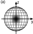
The initial spin state is isotropically distributed along the $x$-direction as is shown in Fig.2(a). After the first interaction, the distribution is a little broadened along the $y$ direction, as Fig.2(b) indicates. This is explained by additional fluctuation imposed by coherent light. In fact, the $y$ components after the first interaction is approximately written as $S_{y}^{\mathrm{(FI)}}=e^{it_{1}H}S_{y}e^{-it_{1}H}\simeq S_{y}+\alpha t_{1}J_{z}S_{x}$ for $\alpha t_{1}J_{z}\ll 1$. Since $S_{z}$ is the BAE variable, the distribution along the $z$ direction does not change at all. After the second interaction, the distribution looks twisted around the $z$-axis and squeezed along the $z^{\prime}$-axis, as Fig.2(c) indicates. Although not clear from the figure, the distribution is also broadened along the $y$-axis as in the case after the first interaction. In fact, the $y$ component after the second interaction is roughly written as $\widetilde{S}_{y}\sim e^{it_{2}H^{\mathrm{(SI)}}}S_{y}^{\mathrm{(FI)}}e^{-it_{2}H^{\mathrm{(SI)}}}\sim S_{y}+\mu S_{z}S_{x}+(\alpha t_{1}J_{z}+\alpha t_{2}J_{y})S_{x}$. By these additional fluctuations imposed by coherent light, the spin state after the second interaction is different from the ideal one-axis twisted state kitagawa. The additional fluctuations would be reduced by use of a polarization squeezed light pulse whose squeezed component is $t_{1}J_{z}+t_{2}J_{y}$, approaching the ideal one-axis twisting interaction of $\mu^{\prime}\to 0$. We mention that the additional fluctuations by light in the method of Ref.hammerer are imposed both on the $y$ and $z$ components, while the $z$ component is squeezed. Therefore, the squeezing parameter does not become small in that scheme.

From Eq.(3) and Eq.(4), we can derive the averages and variances of the spin components. The averages can be calculated as $\langle\widetilde{S}_{x}\rangle=Se^{-\mu^{\prime}/2}\cos^{2S-1}(\mu/2)$ and $\langle\widetilde{S}_{y}\rangle=\langle\widetilde{S}_{z}\rangle=0$, where $\widetilde{\mathbf{S}}$ represents the spin operator after the second interaction. They indicates that the orientation of the mean spin vector remains $(\pi/2,0)$ direction or the $x$-axis, as is shown in Fig.2(c). To characterize a elliptical distribution around the $x$-axis, we define the minor and major axis, say $z^{\prime}$ and $y^{\prime}$, respectively, as is shown in Fig.2(c), so that the variances of whose components $\langle\Delta\widetilde{S}_{z^{\prime}}^{2}\rangle$ and $\langle\Delta\widetilde{S}_{y^{\prime}}^{2}\rangle$ give the minimum and maximum on the $y-z$ plane, respectively. The variances can be calculated as $\langle\Delta\widetilde{S}_{x}^{2}\rangle=S^{2}-\langle\widetilde{S}_{x}\rangle^{2}-S(S-1/2)A/2$ and

where we have set $A=1-e^{-2\mu^{\prime}}\cos^{2S-2}\mu$, and $B=4e^{-\mu^{\prime}/2}\sin(\mu/2)\cos^{2S-2}(\mu/2)$. We can also calculate $\delta$, which is an angle between the directions of the $z^{\prime}$- and $z$-axes, or the $y^{\prime}$- and $y$-axes, as is shown in Fig.2(c), and obtain $\delta=\arctan(B/A)/2$. For $S\gg 1$ and $S^{-1}\ll\mu\sim\mu^{\prime}\ll S^{-1/2}$, we find the approximate value of the variance of the $z^{\prime}$ component

where we have set $\gamma=S\mu/2$, $\gamma^{\prime}=S\mu^{\prime}/2$ and $\beta=S\mu^{2}/4$. Also we find $\langle\widetilde{S}_{x}\rangle\simeq S(1-\beta)$.

To examine the dependence on the interaction strength $\alpha t_{1},\alpha t_{2}$ and the input photon number $2J$, we plot the variances of the $y^{\prime}$ components and the $z^{\prime}$ components as a function of $\mu(=\mu^{\prime})$ in Fig.3(a). We also plot the approximate value for the $z^{\prime}$ components written as Eq.(6).

It is clearly known that the variance of the $z^{\prime}$ component is reduced for small $\mu$, minimized at an optimal value of $\mu$, and becomes large for large $\mu$. It means that too strong interaction or too large photon number deteriorates the squeezing. This is explained by the spherical nature of the spin distribution, and in fact, the variance of the $y^{\prime}$ component is almost saturated at the largest value of $S^{2}/2$ for large $\mu$, which was entirely ignored in the analysis in Ref.hammerer. As a typical value of $\mu$, we introduce $\mu_{\mathrm{half}}$ as the value of $\mu$ to attain $\langle\Delta\widetilde{S}_{z^{\prime}}^{2}\rangle=S/4$, the half variance of the SQL. We also introduce $\mu_{\mathrm{min}}$ as the value to attain the minimum of the $\langle\Delta\widetilde{S}_{z^{\prime}}^{2}\rangle$. We plot the numerical solutions of $\mu_{\mathrm{half}}$ and $\mu_{\mathrm{min}}$ in Fig.3 (b) for the case of $\mu=\mu^{\prime}$. One can see that both $\mu_{\mathrm{half}}$ and $\mu_{\mathrm{min}}$ become small as $S$ increases but they obey different power laws. From Eq.(6), we find $\mu_{\mathrm{half}}\simeq 2S^{-1}$ and $\mu_{\mathrm{min}}\simeq 2(3/2)^{1/5}S^{-3/5}$. We show these approximate solutions in Fig.3 (b), which are in good agreement with the numerical ones. We also find that the squeezing parameter at $\mu=\mu^{\prime}=\mu_{\mathrm{min}}$ becomes $\zeta_{\mathrm{min}}\simeq(2/3)^{1/5}S^{-2/5}$. We note that it is slightly worse than $(1/3)^{1/3}S^{-2/3}$, which is the squeezing parameter for the ideal one-axis twisting, due to the additional fluctuations imposed by coherent light, as is mentioned above.

Finally, we discuss the feasibility of our method. In the following, we consider the case that the shape of the light pulse is a square wave with its peak power $P$ and pulse duration $T$. As in Ref.duan, we assume $\Delta\gg\Gamma$, $\Omega\ll\Delta$, and $rT\ll(S\mu)^{-1}\ll 1$, where $\Delta$ represents the detuning from the resonance frequency, $\Gamma$ the full natural linewidth at half maximum of the transition, $\Omega$ the Rabi frequency, and $r$ the photon scattering rate suter. After some calculations, we obtain $\mu=\mu^{\prime}=rT\sigma_{0}/(2\pi w^{2})$, where $w$ represents the beam waist and $\sigma_{0}$ the photon-absorption cross section of an atom, which can be written as $\sigma_{0}=3\lambda_{0}^{2}/(2\pi)$ with the resonance wavelength $\lambda_{0}$. We note that $\Omega$, $r$ and $\mu$ are exactly the same as $2g\sqrt{2N_{p}/(cT)}$, $4\varepsilon_{a}/T$, and $\kappa^{2}/N_{a}$ in Ref.duan, respectively. The condition to obtain $\mu\geq\mu_{\mathrm{half}}$, or $\zeta\leq 1/2$, can be rewritten as $d_{0}\gtrsim 8(rT)^{-1}$, where $d_{0}=2S\sigma_{0}/(\pi w^{2})$ is the optical depth. We also note that this condition is the same as $\kappa\gtrsim\sqrt{2}$, similar to that of QND measurement duan. Such a condition has been satisfied in several systems, such as atoms in a cell polzik, laser cooled and trapped atom, and so on. The feasibility of our scheme also comes from the simple experimental setup depicted in Fig.1, which is also the great advantage over another scheme in Ref.hammerer. This suggests efficient squeezing can be realized by the current technologies.

As one ideal example, we consider a ytterbium atoms (¹⁷¹Yb) in optical traphonda; takasu, which contains $S=4\times 10^{6}$. The atom collision and the precession due to the stray magnetic field, which causes the transverse relaxation, are well surpressed because it is ultracold fermion and has only nuclear spin 1/2 whose gyromagnetic ratio is about three orders smaller than paramagnetic atoms like alkali metal. From the parameters given in Ref.takasu, $w=3\mathrm{\mu m}$ takasu, $\lambda_{0}=399\mathrm{nm}$ and $\Gamma=2\pi\times 29\mathrm{MHz}$, the light pulse of $\mu=5.4\times 10^{-6}$, for example, is obtained by setting $\Delta=2\pi\times 24$GHz, $P=17\mathrm{nW}$, $T=0.24\mathrm{ms}$, which satisfies the assumptions $\Delta\gg\Gamma$, $\Omega=2\pi\times 21\mathrm{MHz}\ll\Delta$, $rT=4.0\times 10^{-3}\ll(S\mu)^{-1}=4.6\times 10^{-2}\ll 1$. and $J=4.0\times 10^{6}\gg 1$. In this case the squeezing parameter becomes $\zeta=0.08$. We note that the decay constant of the atom number in optical trap is about $4$s ybbec, which is so longer than the the pulse duration $T$ that we can treat the total spin $S$ as a constant. We also note that the length of the atom distribution shuould be adjusted to $L\sim 70\mathrm{\mu m}$ to satisfy the condition of $\pi w^{2}/(\lambda_{0}L)\sim 1$duan, which is easy for atoms in optical trap of crossed configuration.

To avoid the interference between the three steps of the first interaction, the local operation and the second interaction within one pulse, we can use a pluse train, each duration of which is so short that the three steps are separable and the repetition rate is so slow that the pulse number travelling in the path is at most one. Since the each matrix element $\langle S,M|\rho_{S}|S,M^{\prime}\rangle$ would evolve like a geometric progression whose common ratio is $\sigma_{MM^{\prime}}$ for the every pulse as Eq.(2) indicates, and $\sigma_{MM^{\prime}}$ is the power of the mean photon number of the each pulse as Eq.(3) indicates, we can say that the same SSS would be obtained as long as the total mean photon number passed through the atomic ensemble are equal.

References

- (1) M.Kitagawa and M.Ueda, Phys.Rev.A 47, 5138 (1993).
- (2) Y.Takahashi, M.Fujimoto, T.Yabuzaki, A.D.Singh, M.K.Samal,and B.P.Das, in Proceedings of CP Violation and its Origins, edited by K.Hagiwara (KEK Reports, Tsukuba, 1997).
- (3) W.M.Itano, J.C.Bergquist, J.J.Bollinger, J.M.Gilligan, D.J.Heinzen, F.L.Moore, M.G.Raizen, and D.J.Wineland, Phys.Rev.A 47, 3554 (1993).
- (4) D.J.Wineland, J.J.Bollinger, W.M.Itano and D.J.Heinzen, Phys.Rev.A 50, 67 (1994).
- (5) B.Julsgaard, A.Kozhekin, and E.S.Polzik, Nature 413, 400 (2001).
- (6) M.D.Lukin, S.F.Yelin, and M.Fleischhauer, Phys. Rev. Lett. 84, 4232 (2000).
- (7) A.André , L.M.Duan, and M.D.Lukin, Phys.Rev.Lett. 88, 243602 (2002).
- (8) A.Kuzmich, N.P.Bigelow, and L.Mandel, Europhys.Lett. 42, 481 (1998).
- (9) Y.Takahashi, K.Honda, N.Tanaka, K.Toyoda, K.Ishikawa, and T.Yabuzaki, Phys.Rev.A 60, 4974 (1999).
- (10) A.Kuzmich, L.Mandel, J.Janis, Y.E.Young, R. Ejnisman, and N. P. Bigelow, Phys.Rev.A 60, 2346 (1999).
- (11) A.Kuzmich, L.Mandel and N.P.Bigelow, Phys.Rev.Lett. 85, 1594 (2000).
- (12) K.L.Thomsen,S.Mancini, and H.M.Wiseman, Phys.Rev.A 65, 061801 (2002).
- (13) J.M. Geremia, John K. Stockton, and Hideo Mabuchi, Science 304, 270 (2004).
- (14) J. Hald, J.L.Sørensen, C.Schori, and E.S.Polzik, Phys.Rev.Lett. 83, 1319 (1999).
- (15) C.Schori, B.Julsgaard, J.L.Sørensen, and E.S.Polzik, Phys.Rev.Lett. 89, 057903 (2002).
- (16) M.Fleischhauer and M.D.Lukin, Phys.Rev.Lett. 84, 5094 (2000)
- (17) M.Fleischhauer and S.Gong, Phys.Rev.Lett 88, 070404 (2002).
- (18) K.Helmerson and L.You, Phys.Rev.Lett 87, 170402 (2001).
- (19) A.Sørensen, L.M.Duan, J.I.Cirac and P.Zoller, Nature 409, 63 (2001).
- (20) L.M.Duan, A.Sørensen, J.I.Cirac, and P.Zoller, Phys.Rev.Lett. 85, 3991 (2000).
- (21) A.Sørensen and K.Mølmer, Phys.Rev.Lett. 83, 2274 (1999).
- (22) A.S.Sørensen and K.Mølmer, Phys.Rev.A 66, 022314 (2002).
- (23) H.Saito and M.Ueda, Phys.Rev.A 68, 043820 (2003).
- (24) L.Vernac, M.Pinard, and E.Giacobino, Phys.Rev.A 62, 063812 (2000).
- (25) K.Hammerer, K.Mølmer, E.S.Polzik and J.I.Cirac, quant-ph/0312156 (2004).
- (26) L.M.Duan, J.I.Cirac, P.Zoller and E.S.Polzik, Phys.Rev.Lett. 85, 5643 (2000).
- (27) C.Cohen-Tannoudji and J.Dupont-Roc, Phys.Rev.A 5, 968 (1972).
- (28) See for example, Dieter Suter, The Physics of Laser-Atom Interactions, (Cambridge University Press, 1997).
- (29) K.Honda et al., Phys.Rev.A 66, 021401 (2002).
- (30) Y.Takasu et al., Phys.Rev.Lett. 90, 023003 (2003).
- (31) Y.Takasu et al., Phys.Rev.Lett. 91, 040404 (2003).