A comparative study of relative entropy of entanglement, concurrence and negativitypublished in J. Opt. B: Quantum Semiclass. Opt. 6 (2004) 542 –- 548; online at stacks.iop.org/JOptB/6/542

Quantum entanglement is a key resource for quantum information processing but still its mathematical description is far from completeness horodecki-book and its properties are more and more intriguing. In particular, Eisert and Plenio eisert five years ago observed by Monte Carlo simulation of pairs of two-qubit states $\sigma^{\prime}$ and $\sigma^{\prime\prime}$ that entanglement measures (say $E^{(1)}$ and $E^{(2)}$) do not necessarily imply the same ordering of states. This means that the intuitive requirement

can be violated. The problem was then analyzed by others zyczkowski99; virmani; verstraete; zyczkowski02; wei1; wei2; miran1; miran2; mg1. In particular, Virmani and Plenio virmani proved that all good asymptotic entanglement measures are either identical or fail to impose consistent orderings on the set of all quantum states. Here, an entanglement measure is referred to as ‘good’ if it satisfies (at least most of) the standard criteria vedral97a; vedral98; horodecki00 including that for pure states it should reduce to the canonical form given by the von Neumann entropy of the reduced density matrix.

We will study analytically the problem of ordering of two-qubit states imposed by the following three standard entanglement measures.

The first measure to be analyzed here is the relative entropy of entanglement (REE) of a given state $\sigma$, which is defined by Vedral et al vedral97a; vedral98 (for a review see vedral02) as the minimum of the quantum relative entropy $S(\sigma||\rho)={\rm Tr}\,(\sigma\lg\sigma-\sigma\lg\rho)$ taken over the set ${\cal D}$ of all separable states $\rho$, namely

where $\bar{\rho}$ denotes a separable state closest to $\sigma$. We assume, for consistency with the other entanglement measures that $\lg$ stands for $\log_{2}$ although in the original Vedral et al papers vedral97a; vedral98 the natural logarithms were chosen. It is usually difficult to calculate analytically the REE with exception of states with high symmetry, including those discussed in sections 3 and 4. Thus, in general, the REE is calculated numerically using the methods described in, e.g., vedral98; doherty; rehacek. The REE satisfies both continuity and convexity [monotonicity under discarding information, $E(\sum_{i}p_{i}\sigma_{i})\leq\sum_{i}p_{i}E(\sigma_{i})$] donald, but it does not fulfill additivity [$E(\sigma_{1}\otimes\sigma_{2})=E(\sigma_{1})+E(\sigma_{2})$] vollbrecht.

The second measure of entanglement for a given two-qubit state $\sigma$ is the Wootters concurrence $C({\sigma})$ defined as wootters

where the $\lambda_{i}$’s are the square roots of the eigenvalues of ${\sigma}({\sigma}^{(y)}\otimes{\sigma}^{(y)})\sigma^{*}({\sigma}^{(y)}\otimes{\sigma}^{(y)})$ put in nonincreasing order, ${\sigma}^{(y)}$ is the Pauli spin matrix, and asterisk stands for complex conjugation. The concurrence $C({\sigma})$ is monotonically related to the entanglement of formation $E_{\rm form}({\sigma})$ bennett96 as given by the Wootters formula wootters

in terms of the binary entropy $h(x)=-x\lg x-(1-x)\lg(1-x)$. The concurrence and entanglement of formation satisfy convexity wootters; horodecki04. But, to our knowledge, the question about additivity of the entanglement of formation is still open wootters01; horodecki04.

The third useful measure of entanglement is the negativity – a measure related to the Peres-Horodecki criterion peres as defined by

where $\mu_{j}$’s are the eigenvalues of the partial transpose $\sigma^{\Gamma}$ of the density matrix $\sigma$ of the system. Note that for any two-qubit states, $\sigma^{\Gamma}$ has at most one negative eigenvalue. As shown by Audenaert et al audenaert and as subsidiarily by Ishizaka ishizaka04, the negativity of any two-qubit state $\sigma$ is a measure closely related to the PPT entanglement cost as follows:

which is the cost of the exact preparation of $\sigma$ under quantum operations preserving the positivity of the partial transpose (PPT). $E_{\rm PPT}(\sigma)$, similarly to $E_{\rm form}(\sigma)$ and $E(\sigma)$, gives an upper bound of the entanglement of distillation bennett97. As shown by Vidal and Werner vidal, the negativity is a convex function, however $E_{\rm PPT}(\sigma)$ is not convex as a combination of the convex $N(\sigma)$ and the concave logarithmic function. Nevertheless, $E_{\rm PPT}(\sigma)$ satisfies additivity. For a pure state $|\psi_{P}\rangle$, it holds $C(|\psi_{P}\rangle)=N(|\psi_{P}\rangle)$ but $E_{\rm PPT}(|\psi_{P}\rangle)\geq E_{\rm form}(|\psi_{P}\rangle)$, where equality holds for separable and maximally entangled states. For these reasons, we will apply the concurrence and negativity instead of $E_{\rm form}$ and $E_{\rm PPT}$.

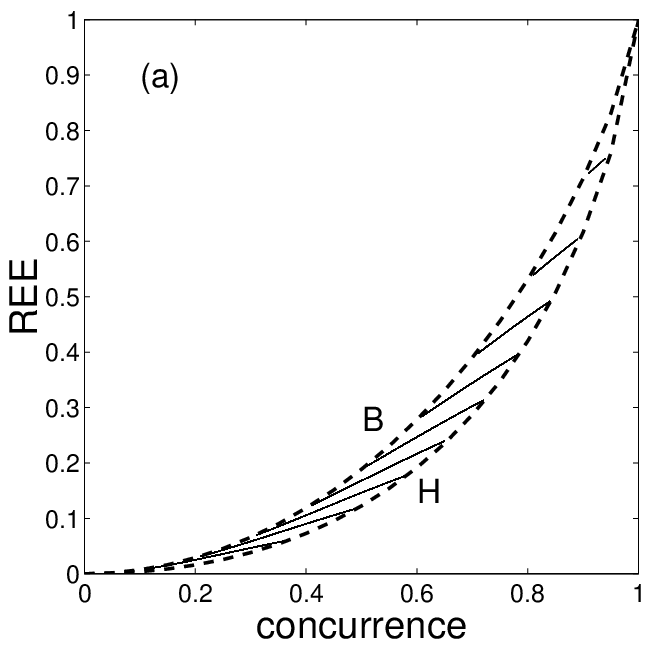
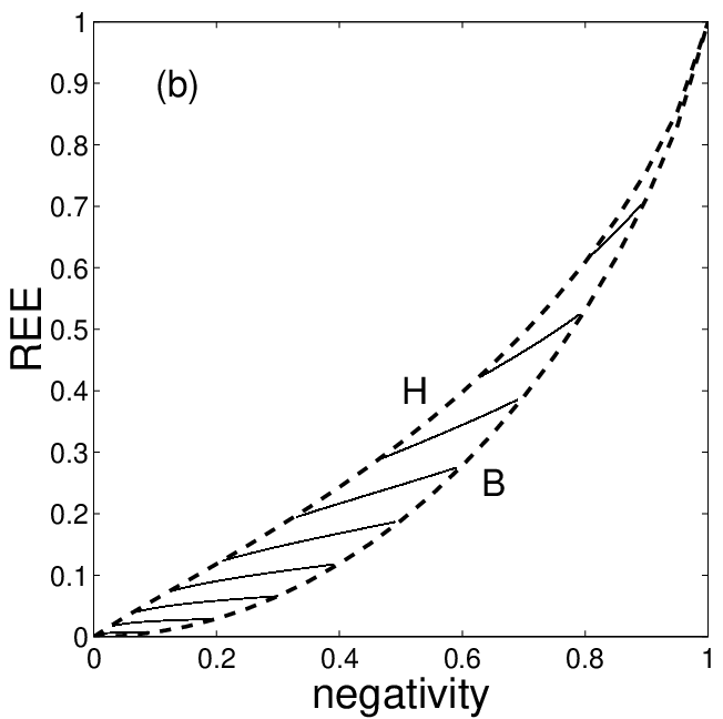
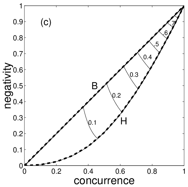
In previous works much attention was devoted to the ordering problem for the concurrence versus the negativity eisert; zyczkowski99; miran1; miran2; mg1. Here, we will study analytically the ordering of two qubit-states imposed by the REE in comparison to the other two measures. But first let us show the violation of condition (1) by numerical simulation. We have generated ‘randomly’ $10^{5}$ two-qubit states according to the method described by Życzkowski et al pozniak; zyczkowski98 and applied, e.g., by Eisert and Plenio eisert. The results are shown in figure 1, where for each generated state $\sigma$ we have plotted $E(\sigma)$ versus $C(\sigma)$, $E(\sigma)$ versus $N(\sigma)$, and $N(\sigma)$ versus $C(\sigma)$. It is worth noting that apparent saw-like irregularity of distribution of states (along the x-axes) is an artifact resulting from the modification of the original Życzkowski et al method. Namely, we have performed simulations sequentially in 10 rounds and during the $k$th round we plotted the three entanglement measures only for those $\sigma$ for which $C(\sigma)$ was greater than $(k-1)/10$. The speed-up of this biased simulation is a result of fast procedures for calculating the negativity or concurrence and very inefficient ones for calculating the REE vedral98; doherty; rehacek; ishizaka04. Our sequential method could be applied since the main goal for generating states was to check efficiently the boundaries of the depicted regions but not the distribution of states.

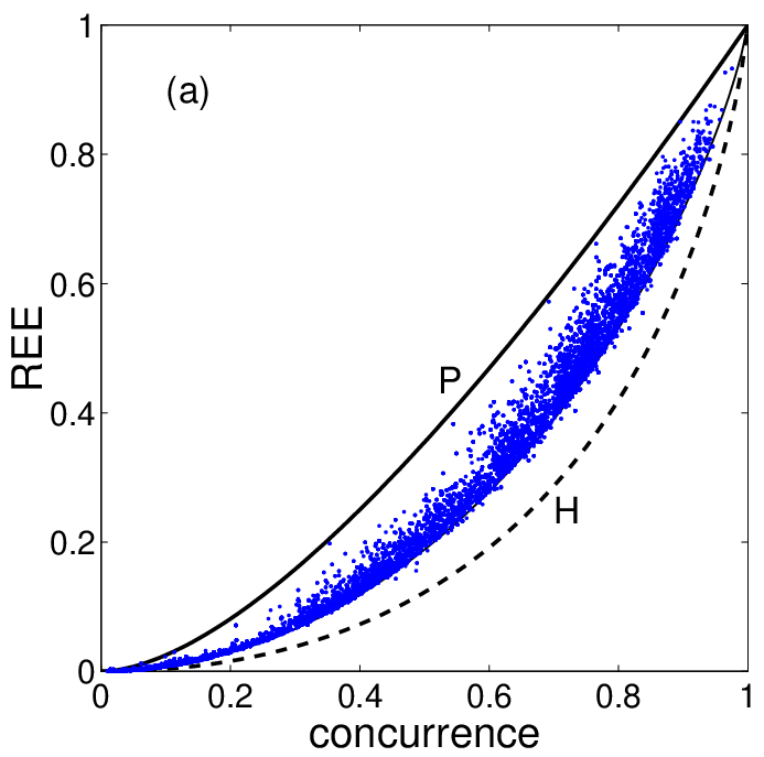
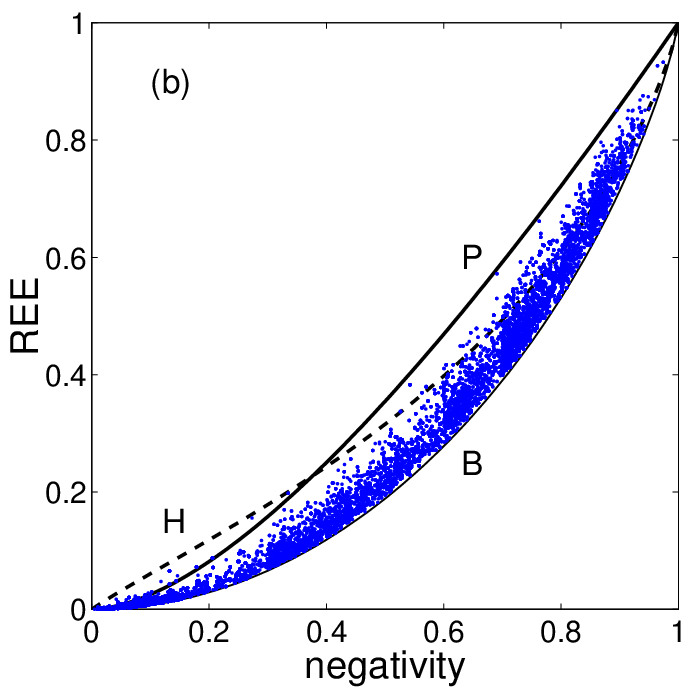
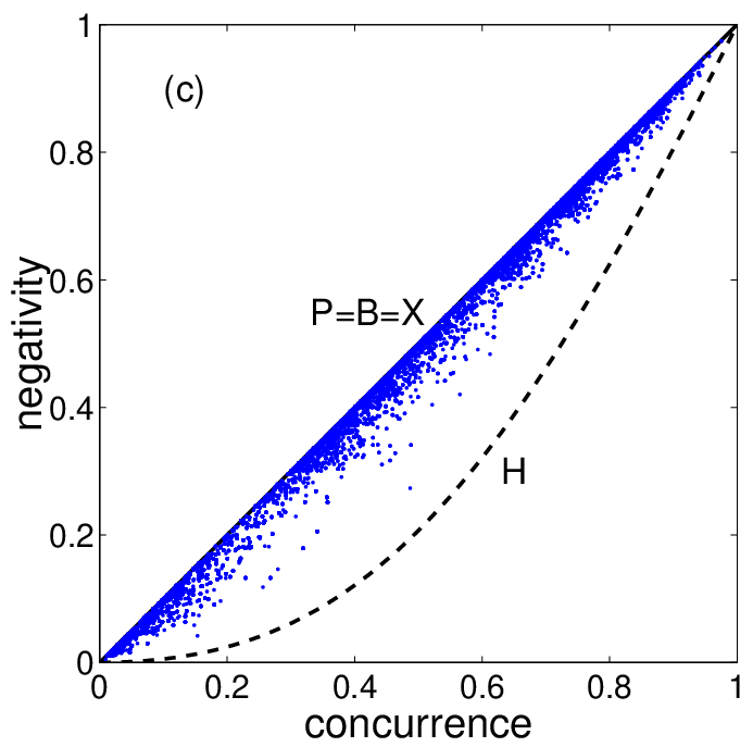
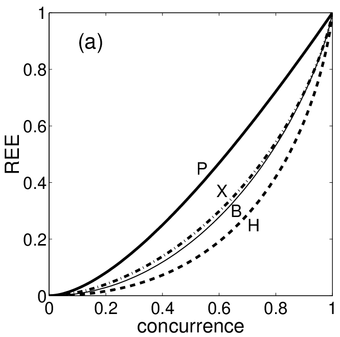
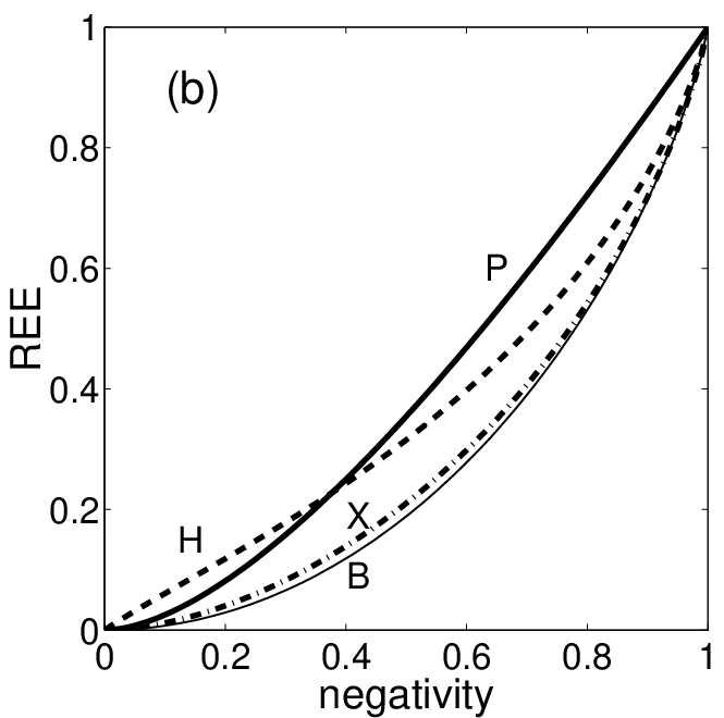
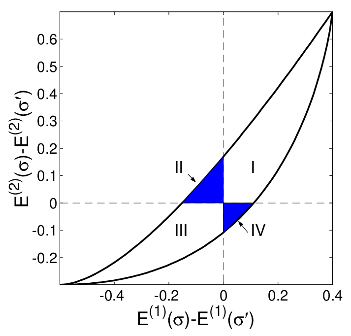
The bounded regions containing all the generated states, as shown in figure 1 and for clarity redrawn in figure 2, reveal the ordering problem as a result of ‘the lack of precision with which one entanglement measure characterizes the other’ wei1. By simply generalizing the interpretation given by us in mg1 to include any two ($E^{(1)}$ and $E^{(2)}$) of the studied entanglement measures, one can conclude that for any partially entangled state $\sigma^{\prime}$ there are infinitely many partially entangled states $\sigma$ for which the Eisert-Plenio condition, given by (1), is violated. To demonstrate this result explicitly for a given state $\sigma^{\prime}$, it is useful to plot $[E^{(2)}(\sigma)-E^{(2)}(\sigma^{\prime})]$ versus $[E^{(1)}(\sigma)-E^{(1)}(\sigma^{\prime})]$ as shown in figure 3. Then the state $\sigma$ corresponding to any point in the regions II and IV is inconsistently ordered with $\sigma^{\prime}$ with respect to the measures $E^{(1)}$ and $E^{(2)}$. On the contrary, the states $\sigma$, corresponding to any point in the regions I and III, and $\sigma^{\prime}$ are consistently ordered by $E^{(1)}$ and $E^{(2)}$.

Probability $P_{\rm ent}$ that a randomly generated two-qubit mixed state is entangled can be estimated as $P_{\rm ent}\approx 0.368\pm 0.002$ zyczkowski98 or $P_{\rm ent}\approx 0.365\pm 0.001$ eisert. However, probability $P_{\rm viol}$ that a randomly generated pair of two-qubit states violates condition (1) for concurrence and negativity is much less than $P_{\rm ent}$ and estimated as $P_{\rm viol}\approx 0.047\pm 0.001$ eisert. Since the numerical analysis of Eisert and Plenio eisert and by the power of the Virmani-Plenio theorem virmani we know about the existence of states violating condition (1). But it is not a trivial task to find analytical examples of such states, especially in the case of the orderings imposed by the REE in comparison to other entanglement measures. We believe that it is not only a mathematical problem of classification of states with respect to various entanglement measures but it can shed more light on subtle physical aspects of the entanglement measures including their operational interpretation. By a comparison given in the next sections, we will find states exhibiting very surprising properties. In particular, we will show that states $\sigma^{\prime}$ and $\sigma^{\prime\prime}$ can have the same negativity, $N(\sigma^{\prime})=N(\sigma^{\prime\prime})$, the same concurrence, $C(\sigma^{\prime})=C(\sigma^{\prime\prime})$, but still different REEs, $E(\sigma^{\prime})\neq E(\sigma^{\prime\prime})$. A deeper analysis of such states can be useful in studies of properties of a given entanglement measure (in this example, the REE) under operations preserving other entanglement measures (here, the entanglement of formation and the PPT-entanglement cost). Thus, we believe that it is meaningful to study analytically violation of condition (1) as will be presented in greater detail in the next sections.

The extreme violation of (1) occurs if one of the states corresponds to a point at the upper bound and the other at the lower bound. Thus, for a comparison of different orderings, it is essential to describe the states at the boundaries.

The upper bounds in figure 1 marked by $P$ correspond to two-qubit pure states

where $a,b,c,d$ are the normalized complex amplitudes. The concurrence and negativity are equal to each other and given by

As shown by Verstraete et al verstraete, the negativity of any state $\sigma$ can never exceed its concurrence [see figure 1(c)], and this bound is reached for the set of states for which the eigenvector of the partial transpose of $\sigma$, corresponding to the negative eigenvalue, is a Bell state. Evidently, pure states belong to the Verstraete et al set of states. For a pure state the REE is equal to the entanglement of formation, thus is simply given by Wootters’ relation (4) since $E(|{\psi}_{P}\rangle)=E_{\rm form}(|{\psi}_{P}\rangle)$. In general, it holds $E_{\rm form}(\sigma)\geq E(\sigma)$ vedral98, and the REE for pure states gives the upper bound of the REE versus concurrence verstraete. We have also conjectured in mg2, on the basis of numerical simulations similar to those presented in figure 1(b), that the upper bound of the REE versus negativity $N$ is reached by pure states for $N\geq N_{0}\equiv 0.3770\cdots$.

Surprisingly, the REE versus $N$ for pure states, can be exceeded by other states if $N<N_{0}$ as was shown in mg2 by the so-called Horodecki states, which are mixtures of the maximally entangled state, say the singlet state $|\psi_{-}\rangle=(|01\rangle-|10\rangle)/\sqrt{2}$, and a separable state orthogonal to it, say $|00\rangle$, i.e. horodecki-book:

for which the concurrence and negativity are given, respectively, by

Verstraete et al verstraete proved that a function of the form (10b) determines the lower bound of the negativity versus concurrence for any state $\sigma$ [see curve H figure 1(c)]. On the other hand, the REE versus concurrence for the Horodecki states is given by vedral98

By replacing $C$ by $\sqrt{2N(1+N)}-N$ in (11), one gets an explicit dependence of $E(\sigma_{H})$ on the negativity $N(\sigma_{H})$ mg2. It was conjectured that the REE for the Horodecki states describes the lower bound of the REE versus concurrence vedral98, as shown by curve H in figures 1(a) and 2(a), and also conjectured mg2 that it gives the upper bound of the REE versus negativity if $N\leq N_{0}$ as seen in figures 1(b) and 2(b) mg2. The ordering violation for any two of the three entanglement measures can be shown for a pair of the Horodecki and pure states, say $\sigma^{\prime}$ and $\sigma$, if one of the states is partially entangled ($0<E^{(1)}(\sigma^{\prime})<1$) and $\sigma$ is properly chosen according to the rule shown in figure 3 with an exception for the following case: If one of the states in the pair of the Horodecki and pure states has the negativity equal to $N_{0}$ then the ordering imposed by the REE and negativity for these states is always consistent as required by condition (1).

The lower bound in figure 1(b) and the upper bound figure 1(c) correspond to the Bell diagonal state (labeled by $B$), given by

with the largest eigenvalue $\max_{j}\lambda_{j}\equiv(1+C)/2\geq 1/2$, where $\sum_{j}\lambda_{j}=1$ and $|\beta_{i}\rangle$ are the Bell states. The negativity and concurrence are the same and given by

thus $\sigma_{B}$, similarly to pure states, belongs to the Verstraete et al set of states maximizing the negativity for a given concurrence. For the Bell diagonal states, the REE versus the concurrence (and the negativity) reads as vedral97a

If $\max_{j}\lambda_{j}\leq 1/2$ then the state is separable, thus $C(\sigma_{B})=N(\sigma_{B})=E(\sigma_{B})=0$. As an example of (12), one can analyze the Werner state werner

where $0\leq C\leq 1$; $I$ is the identity operator of a single qubit. Our choice of parametrization of (1) leads to straightforward expressions for the negativity and concurrence given by (13). The results of our simulation of $10^{5}$ random states presented in figure 1(b) confirm our conjecture in mg2 that the lower bound of the REE versus negativity is determined by the Bell diagonal states. Nevertheless, to our knowledge, this conjecture and the other proposed by Verstraete et al verstraete on the lower bound of the REE versus concurrence have not been proved yet horodecki04. By contrast, it is easy to prove, by applying local random rotations to both qubits bennett96, that the lower bound of the REE versus fidelity is reached by the Bell diagonal states vedral98. It is worth noting that the REE versus concurrence for $\sigma_{B}$ is not extreme as shown by curve $B$ in figure 2(a).

Let us analyze another state corresponding to the upper bound for $N$ versus $C$, but neither reaching the bounds for $E$ versus $C$ nor $E$ versus $N$. The state is defined as a MES, say the singlet state, mixed with $|01\rangle$ as follows:

for which one gets

The eigenvalues of the partially transposed $\sigma_{X}$ are $\{1-C/2,-C/2,C/2,C/2\}$ and they correspond to the eigenvectors given by $\{|01\rangle,|\phi_{+}\rangle,|\phi_{-}\rangle,|10\rangle\}$, where $|\phi_{\pm}\rangle=(|00\rangle\pm|11\rangle)/\sqrt{2}$. Thus, the Verstraete condition for states with equal concurrence and negativity is fulfilled for the state $\sigma_{X}$, as the negative eigenvalue $-C/2$ corresponds to the Bell state. The separable state $\bar{\rho}_{X}$ closest to $\sigma_{X}$ was found by Vedral and Plenio vedral98 as $\bar{\rho}_{X}=(1-C/2)|01\rangle\langle 01|+C/2|10\rangle\langle 10|$, which enables calculation of the following REE:

where $r=1+\sqrt{(1-C)^{2}+C^{2}}$. Although (17) describes the upper bound for $N$ versus $C$, (18) differs from the extreme expressions for $E$ versus $C$ and $E$ versus $N$ given for the pure, Horodecki and Bell diagonal states. Figures 2(a) and 2(b) show clearly the differences.

We will also analyze the states dependent on two parameters defined as

assuming that $C\leq 2\sqrt{A(1-A)}$ to ensure $\sigma_{Y}$ to be positive semidefinite. States of the form, given by (19), can be obtained by mixing a pure state $|\psi_{P}\rangle$ with the separable state $\bar{\rho}_{P}$ closest to $|\psi_{P}\rangle$ mg2. This mixing leaves the closest separable state unchanged as implied by the Vedral-Plenio theorem vedral98. The eigenvalues of the partial transpose of $\sigma_{Y}$ are $\{1-A,A,-C/2,C/2\}$, which correspond to the following eigenvectors $\{|10\rangle,|01\rangle,|\phi_{-}\rangle,|\phi_{+}\rangle\}$, respectively. Thus, the negative eigenvalue $-C/2$ corresponds to the Bell state $|\phi_{-}\rangle$, which implies that $\sigma_{Y}$ belongs to the Verstraete et al set of states with equal negativity and concurrence,

The REE for state (19) reads as

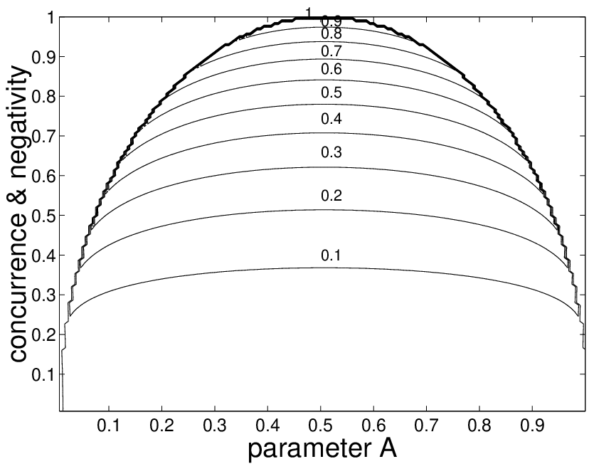
which was obtained with the help of the closest separable state $\bar{\rho}_{P}=A|01\rangle\langle 01|+(1-A)|10\rangle\langle 10|$ given in vedral98. The contour plot of $E(\sigma_{Y})$ is shown in figure 4. The states (19), independent of parameter $A$, are the upper bound states for $N$ versus $C$. By changing $A$, the states (19) transform from the pure states into Bell diagonal states, thus they can become the upper bound states both for $E$ versus $C$ and $E$ versus $N\geq N_{0}$, as well as the lower bound states for $E$ versus $N$. In general, a state corresponding to any point between curves $P$ and $B$ in figures 2(a) and 2(b) can be given by (19).

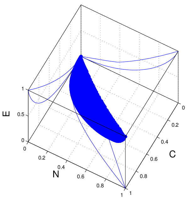
By analyzing pairs of states discussed in the previous section and by applying the rule shown in figure 3 we can easily find analytical explicit examples of states violating condition (1) by any two measures out of the triple, when the third measure is not analyzed. However, the number of classes of state pairs increases to 14, as shown in table 1, on including all possible different predictions of the state orderings imposed by all the three measures simultaneously. The number of classes is given mathematically by permutation with replacement (where the order counts and repetitions are allowed) and equal to $3^{3}$. But we should not count twice the classes defined by opposite inequalities [e.g., class 2 can be equivalently given by $C(\sigma^{\prime})>C(\sigma^{\prime\prime})$, $N(\sigma^{\prime})<N(\sigma^{\prime\prime})$, $E(\sigma^{\prime})>E(\sigma^{\prime\prime})$] since the definition of states $\sigma^{\prime}$ and $\sigma^{\prime\prime}$ can be interchanged. Thus, the number of classes decreases to $(3^{3}-1)/2+1=14$. One can identify all these classes by analyzing pairs of points in the crescent-like solid region in $CNE$ space shown in figure 5 with the familiar projections into the planes $CE$ [see also figure 1(a)], $NE$ [figure 1(b)], and $CN$ [figure 1(c)]. Unfortunately, a graphical illustration of various cross sections of the solid crescent in figure 5 would not be clear enough. Thus, in figure 6, we give a symbolic representation of the 14 classes of table 1 by depicting only small cubes around point $[C(\sigma^{\prime}),N(\sigma^{\prime}),E(\sigma^{\prime})]$ for a given state $\sigma^{\prime}$. In a sense, the cubes are cut inside the solid crescent shown in figure 5.

In the following, we will give explicit examples of the pairs of states satisfying the inequalities listed in table 1. For compact notation we denote

States consistently ordered by all the three measures as required by the Eisert-Plenio condition (1) belong to class 1. The vast majority of the randomly generated pairs of two-qubit states belong to this class. The simplest analytical example is a pair of pure states $|\psi_{i}\rangle=a_{i}|00\rangle+b_{i}|01\rangle+c_{i}|10\rangle+d_{i}|11\rangle$ ($i$=1,2), for which $|a_{1}d_{1}-b_{1}c_{1}|\neq|a_{2}d_{2}-b_{2}c_{2}|$. Similarly, by comparing other pairs of states, to mention $(\sigma_{H}(C^{\prime}),\sigma_{H}(C^{\prime\prime}))$, $(\sigma_{B}(C^{\prime}),\sigma_{B}(C^{\prime\prime}))$ or $(\sigma_{X}(C^{\prime}),\sigma_{X}(C^{\prime\prime}))$ for $C^{\prime}\neq C^{\prime\prime}$, one arrives at the same conclusion. A pair of states from class 2 can be given, e.g., by the Bell diagonal and Horodecki states for slightly different concurrences (or negativities). E.g., if $\sigma_{B}(C=0.5)$ and $\sigma_{H}(C=0.6)$ then $\Delta=[0.1,-0.179,0.003]$, or for the same $\sigma_{B}$ but $\sigma_{H}$ having its negativity equal to $0.4$ then $\Delta=[0.158,-0.1,0.055]$ as required. As an example of the state pair from class 3, we choose the Horodecki and pure states such that their negativities are close to $N_{0}$. E.g., let $\sigma_{H}$ have the negativity $N_{0}-0.1$ and $|\psi_{P}\rangle$ have its coefficients satisfying $2|ad-bc|=N_{0}$ then $\Delta=[-0.187,0.1,0.064]$. By choosing pure state with concurrence $C^{\prime}=0.625\cdots$ and the Horodecki state for $C^{\prime\prime}=0.846\cdots\equiv C_{0}$, we observe that their REEs are the same. Then, an example of the state pair from class 4 can be given by the above pure state and the Horodecki state with its concurrence slightly less than $C_{0}$, say $C(\sigma_{H})=C_{0}-0.02$, which implies that $\Delta=[0.200,0.044,-0.037]$ as required. The classes 1–4 are defined solely by sharp inequalities, and thus they are crucial in our comparison of different state orderings.

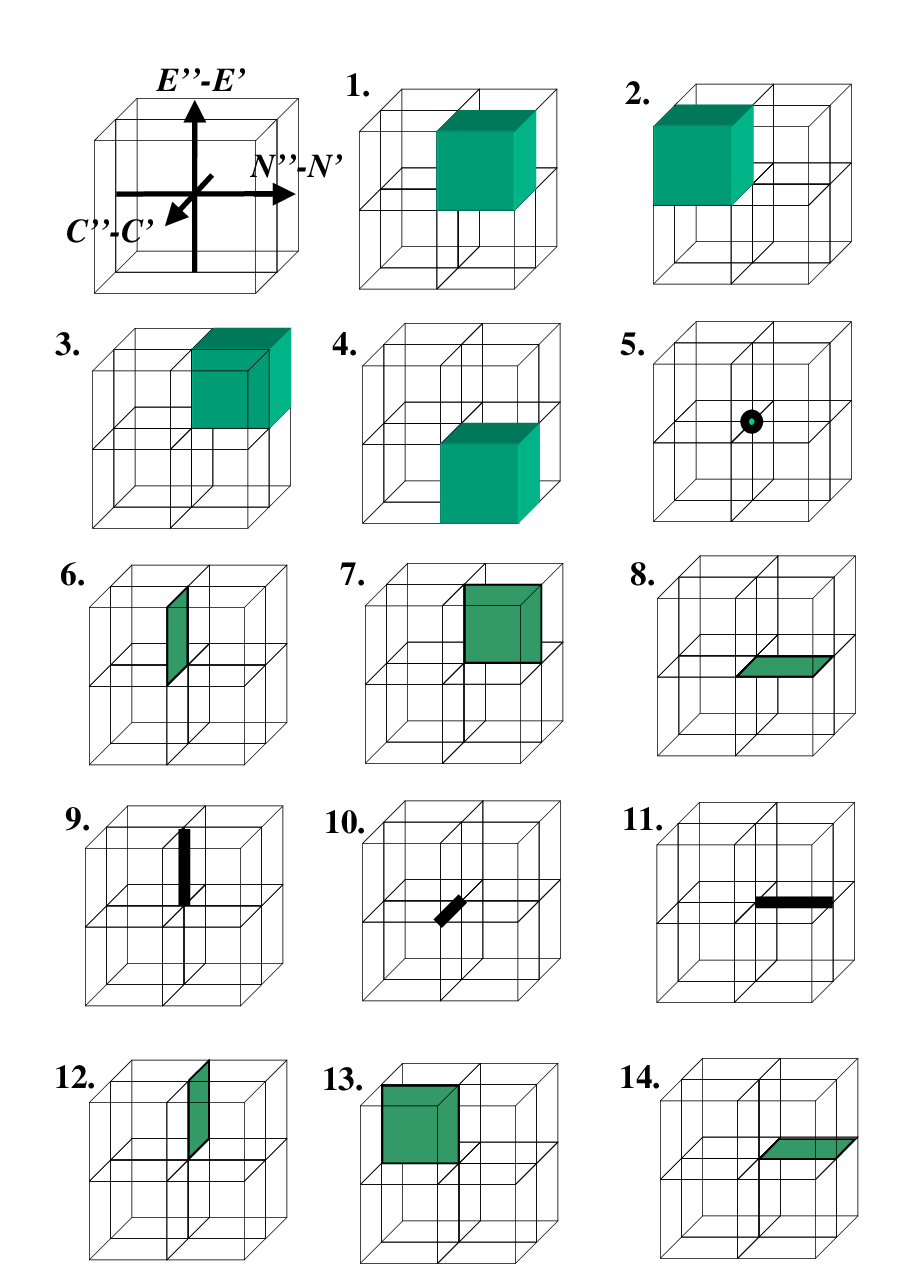
Now, we will present more subtle comparison to include the classes, when some of the entanglement measures are equal to each other for different states. Class 5 is interesting enough to be analyzed separately in the next section. An example of the state pair from class 6 can be given by the Bell diagonal and Horodecki states with the same negativities, say equal to $1/2$, which implies that $\Delta=[0.225,0,0.127]$. Also a member of class 7 can be given by the above states but for the same concurrences, say $C=0.5$, which implies that $-\Delta=[0,0.293,0.066]$. Simple examples of the state pairs from classes 6 and 7 can also be found by considering the following state:

for $N>0$ and $C\in\langle N,\sqrt{2N(N+1)}-N\rangle$, where $\alpha=(C^{2}-N^{2})/(2N)$. The range-limited $C$ ensures semi-definiteness of $\sigma_{Z}$. State (22) can be generated by mixing the Horodecki state $\sigma_{H}$ with the separable state $\bar{\rho}_{H}$ closest to $\sigma_{H}$ given by Vedral and Plenio vedral98 (for details see mg2). We note that the coefficients $C$ and $N$ in (22) are chosen so that

Then, we can write the REE as follows:

where $\beta=\alpha(1+\alpha)/[(1+\alpha)^{2}-C^{2}]$ and $h_{3}(x_{1},x_{2})=-\sum_{i=1}^{3}x_{i}\lg x_{i}$ with $x_{3}=1-x_{1}-x_{2}$. By changing $C$ and $N$ separately, we can obtain $\sigma_{Z}$ with a desired REE. For example, by fixing the negativity, we get the state pair corresponding to class 6, as shown by the contours of constant negativity in figure 7(a). On the other hand, by fixing the concurrence, the resulting states $\sigma_{Z}$ satisfy the conditions for class 7, as presented by the contours of constant concurrence in figure 7(b).

To class 8 belongs a pair of, e.g., the pure state with concurrence $0.625\cdots$ and the Horodecki state with $C=0.846\cdots$, then it holds $E(|\psi_{P}\rangle)=E(\sigma_{H})=0.5$, and $\Delta=[0.220,0.080,0]$ as requested. To find an exemplary member of class 9, one can compare a pure state and any other state from the Verstraete et al set of states (including $\sigma_{B}$, $\sigma_{X}$ or $\sigma_{Y}$) with the same concurrence, which means also the same negativity. For example, for $C(|\psi_{P}\rangle)=C(\sigma_{B})=1/2$ one gets $\Delta=[0,0,0.189]$. As regards class 10, we can compare the pure and Horodecki states with the same negativity $N=N_{0}$, which implies that $E(|\psi_{P}\rangle)=E(\sigma_{H})$. Thus, we have $\Delta=[0.265,0,0]$. Unfortunately, by comparing the states discussed in this section, we have not found examples of the state pairs from classes 11–13. But we can give a few exemplary members of class 14. E.g., by comparing the Bell diagonal state for $C^{\prime}=0.779\cdots$ and the Horodecki state for $C^{\prime\prime}=0.846\cdots$ we find that $E(\sigma_{B})=E(\sigma_{H})=0.5$, while their negativities and concurrences violate condition (1) to the following degrees $\Delta=[0.066,-0.074,0]$. Also by analyzing figure 7(c) for any two points at the same contour of constant REE, we find exemplary state pairs from class 14. Thus, we have presented simple analytical examples of the states satisfying 11 out of 14 classes listed in table 1.

Here, we will analyze examples of inequivalent states $\sigma^{\prime}\neq\sigma^{\prime\prime}$, which have the same degree of entanglement according to $E$, $C$, and $N$, thus corresponding to class 5 in table 1. It is tempting to choose simply two different pure states with their coefficients satisfying $|a_{1}d_{1}-b_{1}c_{1}|=|a_{2}d_{2}-b_{2}c_{2}|$, which guarantees the fulfillment of the equalities required for this class. However, such pure states can be transformed into each other by local operations. To show this, first we note that any pure state, given by (7), can be transformed by local rotations into the superposition $|\tilde{\psi}_{P}(p)\rangle=\sqrt{p}|01\rangle+\sqrt{1-p}|10\rangle$ ($0\leq p\leq 1$), for which the concurrence and negativity are equal to $2\sqrt{p(1-p)}$, as a special case of (8). The same value of these entanglement measures occurs also for $|\tilde{\psi}_{P}(1-p)\rangle$, but this state can be transformed into $|\tilde{\psi}_{P}(p)\rangle$ by applying NOT gate to each of the qubits. Thus, we have shown that pure states are not good examples of the state pairs from class 5. Then, let us choose, e.g., two different Bell diagonal states but with the same largest eigenvalue greater than $1/2$. By virtue of (13) and (14), we conclude that these states have the same degree of entanglement according to the REE, concurrence and negativity. However, as we will show in the following, they can violate the Bell inequality to different degrees.

The maximum possible violation of the Bell inequality in the Clauser-Horne-Shimony-Holt (CHSH) form clauser

for a two-qubit state $\sigma$ is given by horodecki95

Here, ${\cal B}$ is the Bell operator, $\phi_{i},\phi_{i}^{\prime}$ are two dichotomic variables of the $i$th qubit, and ${\cal E}(\phi_{1},\phi_{2})$ is the expectation value of the joint measurement of $\phi_{1}$ and $\phi_{2}$, and so on for the other expectation values. The quantity $M(\sigma)$ is the sum of the two largest eigenvalues of $T_{p}T_{p}^{\dagger}$, where $T_{p}$ is the $3\times 3$ matrix formed by the elements $t_{nm}={\rm Tr}(\sigma\sigma^{(n)}\otimes\sigma^{(m)})$ given in terms of the Pauli matrices $\sigma^{(j)}$. Inequality (25) is satisfied if and only if $M(\sigma)\leq 1$ horodecki95. As shown in miran2 for any pure state $|\psi_{P}\rangle$, the Bell inequality violation parameter $M(\sigma)$ is closely related to the concurrence and negativity as follows:

We find that $M(\sigma)$ for the Bell diagonal state reads as

where subscripts $(i,j,k)$ change over cyclic permutations of $(1,2,3)$. Concluding, the Bell-inequality violation depends on all $\lambda_{i}$’s, while the entanglement measures $E$, $C$, and $N$ depend solely on the largest $\lambda_{i}$. Thus, as an example of the state pair from class 5, we can choose two Bell diagonal states $\sigma^{\prime}_{B}$ and $\sigma^{\prime\prime}_{B}$ with only the largest eigenvalue being the same and greater than $1/2$ for both states, which implies that the states cannot be transformed into each other by LOCC operations but still have the same degrees of entanglement: $E(\sigma^{\prime}_{B})=E(\sigma^{\prime\prime}_{B})$, $C(\sigma^{\prime}_{B})=C(\sigma^{\prime\prime}_{B})$ and $N(\sigma^{\prime}_{B})=N(\sigma^{\prime\prime}_{B})$.

We have analyzed the problem of inconsistency in ordering states with the entanglement measures. The problem was raised by Eisert and Plenio eisert on the numerical example of the concurrence and negativity and then studied by others zyczkowski99; verstraete; zyczkowski02; wei1; wei2; miran1; miran2; mg1. The ordering problem is closely related to existence of the upper and lower bounds of one entanglement measure versus the other verstraete; wei1; mg1; mg2. Here, we presented analytical examples of the pairs of states consistently and inconsistently ordered by the relative entropy of entanglement in comparison to the concurrence and negativity. In particular, we have found examples of the states for which any of the measures imposes order opposite to that given by the other two measures, which corresponds to classes 1–4 in table 1. We have also identified pairs of states with, in particular, (i) the same concurrences and negativities but different REEs (as corresponding to class 9), (ii) the same REEs and negativities but different concurrences (class 10), (iii) the same REEs but different and oppositely ordered concurrences and negativities (class 14), or (iv) states having the same three entanglement measures (class 5), but still violating the Bell-CHSH inequality to different degrees.

Acknowledgments. We are grateful to M Horodecki, P Horodecki, Z Hradil, G Kimura, W Leoński, R Tanaś, F Verstraete, S Virmani, A Wójcik and K Życzkowski for their valuable comments. AG was supported in part by the Polish State Committee for Scientific Research, Contract No. 0 T00A 003 23.

References

- (1) Horodecki M, Horodecki P and Horodecki R 2001 Quantum Information: An Introduction to Basic Theoretical Concepts and Experiments ed G Alber et al (Berlin: Springer) p 151
- (2) Eisert J and Plenio M 1999 J. Mod. Opt. 46 145
- (3) Życzkowski K 1999 Phys. Rev. A 60 3496
- (4) Virmani S and Plenio M B 2000 Phys. Lett. A 268 31
- (5) Verstraete F, Audenaert K M R, Dehaene J, and De Moor B 2001 J. Phys. A: Math Gen. 34 10327
- (6) Życzkowski K and Bengtsson I 2002 Ann. Phys. (N.Y.) 295 115
- (7) Wei T C, Nemoto K, Goldbart P M, Kwiat P G, Munro W J, and Verstraete F 2003 Phys. Rev. A 67 022110
- (8) Wei T C and Goldbart P M 2003 Phys. Rev. A 68 042307
- (9) Miranowicz A 2004 J. Phys. A: Math Gen. 37 7909
- (10) Miranowicz A 2004 Phys. Lett. A 327 272
- (11) Miranowicz A and Grudka A 2004 Phys. Rev. A 70 032326
- (12) Vedral V, Plenio M B, Rippin M A, and Knight P L 1997 Phys. Rev. Lett. 78 2275
- (13) Vedral V and Plenio M B 1998 Phys. Rev. A 57 1619
- (14) Horodecki M, Horodecki P, and Horodecki R 2000 Phys. Rev. Lett. 84 2014
- (15) Vedral V 2002 Rev. Mod. Phys. 74 197
- (16) Doherty A C, Parrilo P A, and Spedalieri F M 2002 Phys. Rev. Lett. 88 187904
- (17) Řeháček J and Hradil Z 2003 Phys. Rev. Lett. 90 127904
- (18) Donald M J and Horodecki M 1999 Phys. Lett. A 264 257
- (19) Vollbrecht K G H and Werner R F 2001 Phys. Rev. A 64 062307
- (20) Wootters W K 1998 Phys. Rev. Lett. 80 2245
- (21) Bennett C H, DiVincenzo D P, Smolin J A, and Wootters W K 1996 Phys. Rev. A 54 3824
- (22) Horodecki P and Horodecki M 2004 private communication
- (23) Wootters W K 2001 Quantum Inf. Comput. 1 27
- (24) Peres A 1996 Phys. Rev. Lett. 77 1413
- (25) [] Horodecki M, Horodecki P, and Horodecki R 1996 Phys. Lett. A 223 1
- (26) Audenaert K, Plenio M B, and Eisert J 2003 Phys. Rev. Lett. 90 27901
- (27) Ishizaka S 2004 Phys. Rev. A 69 020301
- (28) Bennett C H, Brassard G, Popescu S, Schumacher B W, Smolin J A, and Wootters W K 1996 Phys. Rev. Lett. 76 722
- (29) Vidal G and Werner R F 2002 Phys. Rev. A 65 032314
- (30) Poźniak M, Życzkowski K, and Kuś M 1998 J. Phys. A: Math Gen. 31 1059
- (31) Życzkowski K, Horodecki P, Sanpera A, and Lewenstein M 1998 Phys. Rev. A 58 883
- (32) Miranowicz A and Grudka A 2004 Preprint quant-ph/0409009
- (33) Werner R F 1989 Phys. Rev. A 40 4277
- (34) Clauser J F, Horne M A, Shimony A, and Holt R A 1969 Phys. Rev. Lett. 23 880
- (35) Horodecki R, Horodecki P, and Horodecki M 1995 Phys. Lett. A 200 340