Wootters’ distance revisited: a new distinguishability criterium

The problem of measurement is an issue of central importance in quantum theory, that, since the pioneering days of the twenties has given rise to controversies Wheeler. Many of the most astonishing results of quantum mechanics are related to the particular properties of the measurement processes. In recent years, the unique character of quantum measurement has led to a new field of research: quantum information technology cryp. From a formal point of view, a measurement in quantum theory is described by means of an Hermitian operator. If the eigenstates of this operator are $|\phi_{k}\rangle$ and the state of the system to be measured is $|\Psi\rangle=\sum c_{k}|\phi_{k}\rangle$, then, according to the axioms of the quantum theory, the result of the measurement will, with probability $|c_{k}|^{2}$, be the corresponding eigenvalue $a_{k}$, represented physically by an appropriate state of the measuring device $\cal{A}$.

A close related theme is that of the distinguishability between states, that is, just how can we discern between two states $|\Psi^{(1)}\rangle$ and $|\Psi^{(2)}\rangle$ of a given physical system by using the measuring device $\cal{A}$. In a seminal paper, Wootters investigated this problem and introduced a “distinguishability-distance” between pure states in the associated Hilbert space Wootters. Braunstein and Caves extended this distance to density operators for mixed states Caves. Wootters distinguishability-criterium can be established, within the framework of probability theory (independently of any quantum interpretation), in the following way Wootters: two probability distributions, say, $p^{(1)}=(p_{1},p_{2},\ldots,p_{N})$ and $p^{(2)}=(q_{1},q_{2},\ldots,q_{N})$ are distinguishable after $L$ trials ($L\rightarrow\infty$) if and only if the condition

with $\delta p_{i}=p_{i}-q_{i}$, is satisfied. This distinguishability-criterium involves a distance defined over the space of probability distributions

Statisticians call to the square of this form the $\chi^{2}$ distance. Wootters maps this distance into the associated Hilbert space and establishes a correspondence with the usual notion of distance between states in Hilbert’s space.

In addition to its relevance with regards to the distinguishability issue, the concept of distance between different states in a Hilbert space plays an important role in a diversity of circumstances

• •

  the study of the geometric properties of the quantum evolution sub-manifold Anandan; Abe,

• •

  in discussing squeezed coherent states or generalized coherent spin states Kwek,

• •

  in ascertaining the quality of approximate treatments Casas1.

It has recently been recognized that the concept of distinguishability is basic to manipulate information in the sense that being able to discern between different physical states of a given system allows one to determinate just how much information can be encoded into that system, so that the notion of distinguishability builds a bridge between quantum theory and information theory Vedral.

In this work we will try to strengthen this connection by investigating the relation between Wootters’ distance and a suitable metric for the probability-distributions’ space that is used in information theory: the Jensen-Shannon divergence (JSD). Recently, the JSD has been exhaustively studied in different contexts Grosse. It has many interesting interpretations, both in the framework of information theory as in the context of mathematical statistics. One of its basic properties is that its square root is a true metric in the probability-distributions’ space, i.e., its square root is a distance that verifies the triangle inequality Endres. This fact is quite relevant, since metric properties are crucial for the application of many important convergence theorems that one needs when iterative algorithms are studied.

The purpose of this paper is twofold:

1. 1.

   first, we pursue a pedagogical objective by reviewing some distances and metrics commonly used in quantum theory. Even though many of the results presented here are known, they are not always presented from an unified perspective, at least in physics literature,

2. 2.

   second, we formulate a distinguishability criterium for quantum mechanics based on the JSD.

Finally, some conclusions are drawn.

Let $s_{X}(p^{(1)},p^{(2)})$ be a distance defined on the space of probability distributions $X_{N}^{+}$, that is, an application from $X_{N}^{+}\times X_{N}^{+}$ into $\Re$ such that is symmetric and $s_{X}(p^{(1)},p^{(2)})=0$ if and only if $p^{(1)}=p^{(2)}$. One can associate to $s_{X}(p^{(1)},p^{(2)})$ a distance in the space ${\cal{H}}^{n+1}$, $s_{\cal{H}}^{\cal{A}}(|\Psi^{(1)}\rangle,|\Psi^{(2)}\rangle)$ through the application $\mathcal{F}_{\cal{A}}$. Let us note that this distance depends upon the measuring instrument $\cal{A}$. Our objective is to find a representative distance of $s_{X}(p^{(1)},p^{(2)})$ in Hilbert’s space independently of the basis $|\phi_{k}\rangle$. This will be attained by looking for the maximum of the associated distance $s_{\cal{H}}^{\cal{A}}$. We discuss some examples below. The pertinent distances are given proper names (e.g., Wootters), according to common usage.

Notation remark: We will use the following notation: $s_{X}$ denotes a distance defined over $X_{N}^{+}$; $s_{\cal{H}}^{\cal{A}}$ denotes the corresponding distance over ${\cal{H}}^{n+1}$ obtained from the correspondence induced by application ${\cal{F}_{\cal{A}}}$; $S_{\cal{H}}$ denotes the maximum of $s_{\cal{H}}^{\cal{A}}$.

Information theoretic measures allow one to build up quantitative entropic divergences between two probability distributions. A common entropic measure is the Kullback-Leibler divergence:

This distance, however, is i) not symmetric, ii) unbounded, and iii) not always well defined. To overcome these limitations Rao and Lin introduced a symmetrized version of the Kullback-Leibler divergence the Jensen-Shannon divergence (JSD), which is defined as

where $H(p)=-\sum_{i}p_{i}\ln p_{i}$ stands for Shannon‘s entropy Rao,Lin.

The minimum of the JSD occurs at $p^{(1)}=p^{(2)}$ and its maximum is reached when $p^{(1)}$ and $p^{(2)}$ are two distinct deterministic distributions. In this case $s_{X}^{JS}=ln2$. As it was mentioned previously, one of the JSD main properties is that of being the square of a metric. A proof of this fact can be found in reference Endres. Alternatively, this can be proved starting from some classical results of harmonic analysis due to Schoenberg Schoe,Berg. The basic property of the JSD that makes Schoenberg theorem applicable is that $s_{X}^{JS}$ is a definite negative kernel, that is, for all finite collection of real number $(\zeta_{i})_{i\leq N}$ and for all corresponding finite sets $(x_{i})_{i\leq N}$ of points in $X_{N}^{+}$, the implication

is valid Tops1.

Another consequence of Schoenberg’s theorems is that the metric space $(X_{N}^{+},\sqrt{s_{X}^{JS}})$ can be isometrically mapped into a subset of a Hilbert space. This result establishes a connection between information theory and differential geometry Tops2, which could have interesting consequences in the realm of quantum information theory.

Consider once again the states $|\psi\rangle$ and $|\eta\rangle$ given by (II.4) in order to evaluate the JSD between the concomitant probability distributions $p^{(1)}(|\psi\rangle),\,\,p^{(2)}(|\eta\rangle)$. By doing so we are evaluating the associated distance in Hilbert’s space $s_{\cal{H}}^{JS,{\cal{A}}}$ between the states $|\psi\rangle$ and $|\eta\rangle$. Expanding the pertinent JSD in $dp_{i}$-terms, one easily ascertains that the first non-vanishing contributions are the quadratic ones

which coincides with (a half of) the Fubini-Study (30) instance up to this order in $dp_{i}$. Up to same order a similar relation exits between the JSD and both the Wootters’ and the Bhattacharyya’ distances, that is

which can be easily checked by inspection. Incidentally, it is worth mentioning that, when we have a continuous probability distribution $p(x)$, the JSD between $p(x)$ and its shifted version $p(x+\delta)$ is related to the Fisher information measure $I$ through the expression

with

Equations (35) have been established up to second order in $dp_{i}$. Let us proceed to higher orders. To do this let us consider a binary system (a generalization to a system with a greater number of states is straightforward). Let $p^{(1)}=(p,q)$ and $p^{(2)}=(p+dp,q-dp)$ with $p+q=1$ two neighboring probability distributions and evaluate the pertinent JSD up to order $dp^{4}$. We get

In turn, the corresponding Wootters’ distance squared, up to the same order is

We detect coincidence between (38) and (39) up to order $dp^{3}$. The fourth order difference equals $\frac{1}{192}$. In other words, the relation

can be established up to third order in $dp$. Figure 1 shows how $s_{X}^{JS}$ and $\frac{(s_{X}^{W})^{2}}{2}$ approache one to each other for $p^{(1)}\approx p^{(2)}$. We took $p^{(1)}=(a,1-a)$ and $p^{(2)}=(b,1-b)$ and evaluated the corresponding distances as a function of $b$ by fixing $a=0.5$.

Going back to Wootters’ distinguishability criterium (1), with equation (40) in mind, we are in a position to enunciate an alternative criterium: two probability distributions $P^{(1)}$ and $P^{(2)}$ are distinguishable after $L$ trials ($L\rightarrow\infty$) if and only if

There exist formal arguments in favor of this last statement, namely i) $(s_{X}^{JS})^{1/2}$ is a true metric for the space $X_{N}^{+}$ and ii) this criterium is established in terms of an information theoretic quantity, the JSD. Obviously inequality (41) is equivalent to inequality (1) for two distributions “close” enough.

In the context of section II the following question emerges: what metric is the representative of $s_{X}^{JS}$ in Hilbert’s space ${\cal{H}}^{n+1}$? Equivalently: what is the maximum of the metric $s_{\cal{H}}^{JS,{\cal{A}}}$? In this case it is difficult (or impossible) to obtain an analytical expression for both metrics, $s_{\cal{H}}^{JS,{\cal{A}}}$ and its upper bound $S_{\cal{H}}^{JS}$. Anyway, it is possible to deduce an upper bound for $s_{\cal{H}}^{JS}$. Let us consider a Hilbert space of dimension 2D and let $|\Psi^{(1)}\rangle$ and $|\Psi^{(2)}\rangle$ be two arbitrary, normalized states (the extension to a greater number of dimensions is straightforward). We set $|\langle\Psi^{(1)}|\Psi^{(2)}\rangle|=\cos\varphi$ for $\varphi\varepsilon[0,\pi/2]$, that is, $\varphi$ is the Wootters distance between $|\Psi^{(1)}\rangle$ and $|\Psi^{(2)}\rangle$.

Let $\{|\phi_{i}\rangle\}_{i=1}^{2}$ be an orthonormal basis for ${\cal{H}}^{2}$. Any other orthonormal basis $\{|\tilde{\phi}_{i}\rangle\}_{i=1}^{2}$ can be related to $\{|\phi_{i}\rangle\}$ via the rotation

with $\theta\varepsilon[0,2\pi]$. We set $p_{i}^{(j)}\equiv|\langle\phi_{i}|\Psi^{(j)}\rangle|^{2}$ and $\tilde{p}_{i}^{(j)}(\theta)\equiv|\langle\tilde{\phi}_{i}(\theta)|\Psi^{(j)}\rangle|^{2}$. Also, $\langle\phi_{i}|\Psi^{(j)}\rangle=\sqrt{p_{i}^{(j)}}e^{i\alpha_{i}^{(j)}}$ (via application of (7)). A little algebra then leads to

and

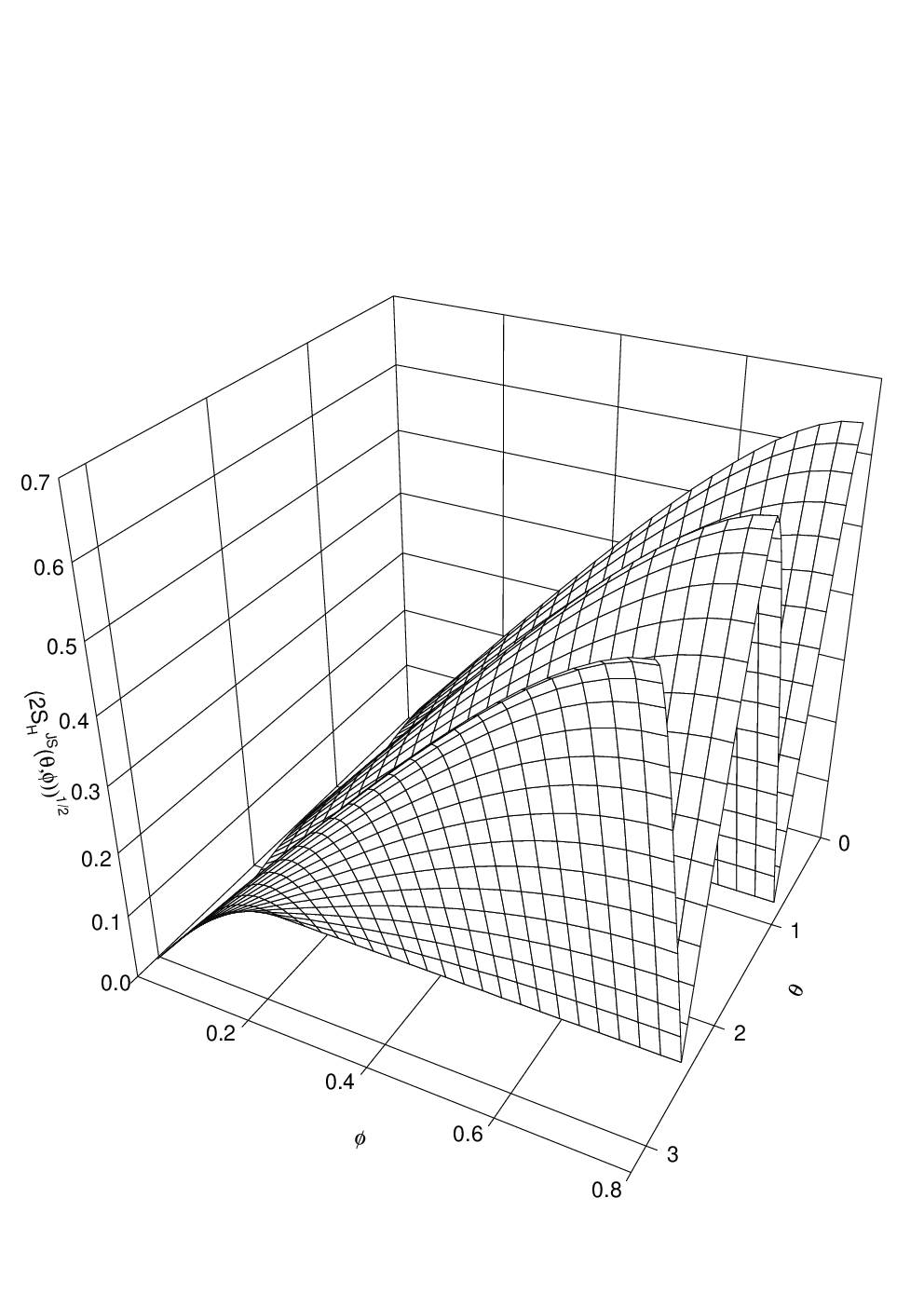
with $\alpha_{i}^{(j)}$ are real numbers. Moreover, $\tilde{p}_{2}^{(1)}=1-\tilde{p}_{1}^{(1)}$ y $\tilde{p}_{2}^{(2)}=1-\tilde{p}_{1}^{(2)}$. Without loss of generality we can take $|\phi_{1}\rangle=|\Psi^{(1)}\rangle$, so that $p_{1}^{(1)}=1$, $\alpha_{1}^{(1)}=0$, $p_{2}^{(1)}=0$,$\sqrt{p_{1}^{(2)}}=\cos\varphi$ y $\sqrt{p_{2}^{(2)}}=\sin\varphi$. Thus, we can compute $\sqrt{2s_{\cal{H}}^{JS,\tilde{\phi}}(\tilde{p}^{(2)},\tilde{p}^{(1)}})$ as a function of $\theta$. Figure 2 plots such a function for different $\varphi-$values. Figure 3 depicts a 3D-plot of $\sqrt{2s_{\cal{H}}^{JS,\tilde{\phi}}}$ as a function of $\theta$ and $\varphi$. In both cases we put $\alpha_{2}^{(1)}=\alpha_{1}^{(2)}=\alpha_{2}^{(2)}=0$.

Out of these figures we conclude that Wootters’ distance ($\varphi$) is an upper bound to $\sqrt{2s_{\cal{H}}^{JS,\tilde{\phi}}(\tilde{p}^{(2)},\tilde{p}^{(1)}})$. For $\varphi\rightarrow 0$, both quantities tend to coincide. In other words, we can state the inequalities

for any measure device $\cal{A}$.

Inequalities (45) allow us to conclude that $S_{\cal{H}}^{W}(|\Psi^{(1)}\rangle,|\Psi^{(2)}\rangle)$ “represents” (as the maximum, that is as the lowest upper bound) to $\sqrt{2s_{\cal{H}}^{JS,{\cal{A}}}}$ in the Hilbert space. Furthermore two states distinguishable under the “Jensen-Shannon criterium” are obviously distinguishable under the Wootters’ ones.

We have proposed an alternative distinguishability criterium for quantum states. This distinguishability criterium is established in terms of an information theoretical quantity: the JSD, that exhibits many interesting properties, such as a metric character and its boundedness. This provides for a better formal context. In some sense we feel that the JSD divergence could be taken as a unified measure of distinguishability in the framework of quantum information theory.

In the present work we focused on the case of pure states. An extension to mixed states can be easily attained. In fact, by replacing in eq.(32) the Shannon entropy by the von Neumann entropy, $H_{N}(\rho)=-{\mathrm{Tr}}(\rho\ln\rho)$, we can evaluate the JSD between two states described by the density operators $\rho_{1}$ and $\rho_{2}$:

Remarkably, this quantity is always well defined unlike the corresponding Kullback-Leibler divergence that requires that the support of $\rho_{1}$ is equal to or larger than that of $\rho_{2}$ Lindblad. A more detailed study of the properties of JSD for mixed states will be presented elsewhere.

Finally it is worth to mention that the JSD can be also interpreted in a Bayesian probabilistic sense. In fact, the JSD gives both lower and upper bounds to Bayes’ probability error. Therefore, it deserves careful scrutiny in the light of some alternative quantum descriptions Fuchs.

AKNOWLEDGMENT

We are grateful to Secretaria de Ciencia y Tecnica de la Universidad Nacional de Córdoba for financial assistance. AM is a fellowship holder of SECYT-UNC and PWL and AP are members of CONICET. This work was partially supported by Grant BIO2002-04014-C03-03 from Spanish Goverment.

References

- (1) A. Wheeler and W. Zurek, “Quantum Theory and Measurement”, Princeton University Press, Princeton (1983).
- (2) N. Gisiu, G. Ribordy, W. Trittel and H. Zbinden, Rev. Mod. Phys. 74, 145-195 (2002).
- (3) V. Vedral, Rev. Mod. Phys. 74, 197-234 (2002).
- (4) W. Wootters, Phys. Rev D 23, 357 (1981).
- (5) S. Braunstein and C. Caves, Phys. Rev. Lett. 72 3439 (1994).
- (6) J. Anandan and Y. Aharonov, Phys. Rev. Lett. 65, 14, 1697 (1990).
- (7) S. Abe, Phys. Rev. A, 48, 4102 (1993).
- (8) L.C. Kwek, CH Oh and Xiang-Bin Wang, J. Phys. A: Mathematical and General 32, 6613 (1999).
- (9) M. Ravicule, M. Casas and A. Plastino, Phys. Rev. A, 55, 1695 (1997).
- (10) I. Grosse, P. Bernaola-Galvan, P. Carpena, R. Roman Roldan, J. Oliver y H.E. Stanley, Phys. Rev. E, 65 041905 (2002).
- (11) D. Endres and J. Schindelin, IEEE Trans. Inf. Theory, 49, 7, 1858 (2003).
- (12) D. Brady and L. Hughston, Geometric Issues on the Foundations of Science. Eds. S.A. Huggett, L. Mason, K. Tod, S.-T. Tsou and N. Woodhouse, Oxford University Press,
- (13) A. Bhattacharyya Bull. Calcutta Math. Soc., 35, 99 (1943).
- (14) C. Rao, “Differential Geometry in Statistical Inference”, IMS-Lectures Notes, 10, 217 (1987).
- (15) J. Lin, IEEE Trans. Inf. Theory 37,1, 145 (1991).
- (16) I.J. Schoenberg, Trans. Am. Math. Soc. 44, 3 (1938).
- (17) C. Berg, J. Christensen and P. Ressel, Harmonic Analysis on Semigroups, Springer-Verlag, New York (1984).
- (18) F. Topsøe, “Inequalities for the Jensen-Shannon Divergence”. Draft available at http://www.math.ku.dk/topsoe/.
- (19) B. Fuglede and F. Topsoe, “Jensen-Shannon Divergence and Hilbert space embedding´”. Draft available at http://www.math.ku.dk/topsoe/.
- (20) G. Lindblad, Comm. Math. Phys. 33, 305 (1973).
- (21) C. Caves, C. Fuchs and R. Schack, Phys. Rev. A 65(2), 022305 (2002).